Comparing Hard and Fuzzy C-Means for Evidence-Accumulation Clustering

Abstract—There exist a multitude of fuzzy clustering

algorithms with well understood properties and benefits in various applications. However, there has been very little analysis on using fuzzy clustering algorithms to generate the base clusterings in cluster ensembles. This paper focuses on the comparison of using hard and fuzzy c-means algorithms in the well known evidence-accumulation framework of cluster ensembles. Our new findings include the observations that the fuzzy c-means requires much fewer base clusterings for the cluster ensemble to converge, and is more tolerant of outliers in the data. Some insights are provided regarding the observed phenomena in our experiments.

I. INTRODUCTION

LUSTERING is an unsupervised process of identifying underlying groups or structures in a set of patterns without the use of class labels. There have been a large set of clustering algorithms (see [1], [2] for reviews). Different methods, however, have their limitations in terms of data characteristics that can be processed and types of clusters that can be found. As it is unlikely that a good "universal" clustering method can be found, a recent trend is the use of cluster ensembles which, generally speaking, represent methods that combine the information from multiple clusterings (i.e., partitions of the data into clusters) in order to obtain a new, and hopefully better, clustering. The basic assumption of cluster ensemble here is that the combined clustering is likely to be more robust, more stable, and more representative of the structures/groupings of the data. This approach is inspired by classifier ensembles, and is identified in [3] as one of three major frontiers of clustering techniques in recent years. Some representative works in this area include [4]-[10]. Many results in these papers have indicated improved clustering results compared to the results of single clustering runs.

Ensemble clustering techniques consist of three main components:

z The method used to obtain the individual clusterings (also called base clusterings in this paper), including how diversity (i.e., the differences among them) is introduced. For the individual clusterings, k-means related methods are most common, as well as EM. Diversity can be introduced through random initialization for both methods above, such as in [5] and [11]. Diversity through the projection to random subspaces is suitable for high-dimensional data [6]. Different order of data presentation is a source of diversity for on-line clustering

Tsaipei Wang is with the Department of Computer Science, National Chiao Tung University, Hsinchu, Taiwan (e-mail: wangts@cs.nctu.edu.tw).

[12]. We can also obtain each base clustering from a different subset of the data. This is a natural choice when we want to obtain a combined clustering using data from multiple sites without first putting them all in one place [13].

z The representation that combines the information from multiple base clusterings. The most common form is a co-association matrix, where pairwise similarities among the patterns are derived from the individual clusterings. Other methods include hypergraphs [4] and bipartite graphs [7]. The collection of all the prototypes in all the base clusterings is very compact and especially useful when the data set is very large [13].

z The extraction of the final (combined) clustering from the representation above. Here the applicable methods depend on the form of the representation. For example, graph partitioning algorithms are used for graph-based representations. For the co-association matrix, k-means based methods [14], spectral clustering [15], graph partitioning [4], and hierarchical agglomeration [5][6] have all been used.

Cluster ensembles based on the evidence-accumulation clustering (EAC) [5] have attracted a lot of attention recently, probably because it is easy to understand conceptually and to implement, and also because it is applicable to problems where the true number of clusters is unknown. The original EAC builds a co-association matrix using outcomes of multiple randomly initialized HCM runs with mostly over-specified numbers of clusters, and extracts the combined clustering using hierarchical agglomeration with single or average linkage. EAC has been extended to clustering patterns with mixed categorical and numerical features [15]. The stability of EAC with single-linkage is analyzed in [17]. However, one known drawback of EAC, as well as other methods that use co-association matrices, is the large number of base clusterings required to achieve reliable results. For example, experiments in [5] indicate that 50 or more base clusterings are usually needed to reliably identify the true number of clusters.

Most cluster ensemble techniques, including the original EAC, are based on crisp (hard) clusterings, and therefore are not able to incorporate ambiguities in the data. Some existing works that do use soft clusterings, such as [6] and [8], do not actually compare the clustering results using hard or soft base clusterings. There have also been a few applications of soft cluster ensembles (ensembles with soft base clusterings), such as [18] and [19], but these contain no comparison between corresponding crisp and soft cluster ensembles.

Comparing Hard and Fuzzy C-Means for Evidence-Accumulation

Clustering

Tsaipei Wang, Member, IEEE

Punera and Ghosh [11] compared the performance of ensembles of crisp or soft base clusterings obtained using EM; a crisp clustering is obtained by assigning each pattern to the most likely cluster in the corresponding soft clustering. The combination methods tested include Cluster-based Similarity Partitioning Algorithm (CSPA) [4], Meta-CLustering Algorithm (MCLA) [4], and Hybrid Bipartite Graph Formulation (HBGF) [7]. The evaluation is based on normalized mutual information (NMI) with the ground-truth partition. The conclusion in [11] is that using soft clusterings does improve the correctness of the final clusterings. Avogadri and Valentini [14] used FCM to generate the base clusterings; the corresponding hard clusterings are obtained by either alpha-cut or assigning each pattern to the most likely cluster. Their results also indicated better accuracy of fuzzy versus hard base clusterings, but only for a synthetic data set of 3 well-separated hyperspherical clusters. Both [11] and [14] study only the cases where the true number of clusters is known and used as the number of clusters for all the base clusterings as well as the combined clustering.

In this paper, we focus on the performance comparison of EAC using either HCM or FCM as the base clustering generator. These two versions are subsequently denoted as hEAC and fEAC in this paper. We specifically analyze two aspects that have not been analyzed in the literature: The speed of convergence in terms of the number of base clusterings needed to produce a stable combined clustering, and how hEAC and fEAC are affected by noise points in the data. For the remainder in this paper, we start with the description of both the crisp and soft versions of EAC, followed by the description of our experiments and results, and the conclusion.

II. EVIDENCE-ACCUMULATION CLUSTERING A. Crisp Evidence-Accumulation Clustering

Our description here follows the algorithm in [5]. Assume that the set X ={x1, x2, …, xn} contains n patterns (data

points). Let P ={C1, C2, …, Ck} be a crisp clustering

(partition) of X. Here k is the number of clusters in P, and the clusters, C1, C2, …, Ck, are disjoint non-empty subsets of X,

and the union of all the clusters in P is the same as X. For a data set X it is possible to obtain many different P. Let a cluster ensemble consists of N clusterings of X: P1, P2, …, PN.

As we allow each individual clustering to have a different number of clusters, we use kq to represent the number of

clusters in Pq (1≤q≤N).

A nxn co-association matrix, S(q) = [sij(q)], is computed for

each clustering Pq. To determine its elements, let ci (q)

represent the cluster index of xi in Pq. Then sij (q)

is given by the following formula:

¦

≤ ≤q N

N1

The co-association matrix is a similarity matrix that can then be fed into various algorithms for relational data clustering. Hierarchical agglomeration with single or average linkage is the method of choice in EAC because it does not require a pre-specified number of clusters. Such algorithms generate a hierarchy of clusterings. When the number of clusters is unknown, the maximum-lifetime criterion is used to select a clustering from the hierarchy. We use kf to

represent the number of clusters in this selected clustering.

B. Soft Evidence-Accumulation Clustering

Similar to [11], here the term "soft" refers only to the base clusterings in an ensemble, meaning that these individual clusterings are soft. However, the combined clustering may still be crisp. This is the case in this paper as we follow the method in [5] and use hierarchical agglomeration to generate the combined clustering.

A soft clustering is represented by a partition (or membership) matrix U = [uti], where uti is the membership of

xi in the tth cluster. For a probabilistic clustering, the

membership matrix satisfies the condition 1 , 1 = ∀

_¦

= k t ti u i . (3) Here k is the number of clusters. Such a clustering can be obtained with EM, which is the method used in [6] and [11], or FCM, which is the method used in [14] and in this paper.

A straightforward extension of (1) for computing co-association matrix from a membership matrix is [6]

¦

= = q k t q tj q ti q ij u u s 1 ) ( ) ( ) ( , (4) or when put in matrix form,

( )

_q T

q

q) ( ) ( )

( _{U U}

S = . (5)

The superscripts (q) in U(q) and uti (q)

indicate that the memberships are for the qth clustering within the ensemble. This form of aggregating the memberships is just the algebraic product form of t-norms in fuzzy set theory. It is used in [6] and [14], and is the method used in our experiments. Other forms of t-norms can also be used. An example is the minimum, as used in [13]:

¦

= = q k t q tj q ti q ij u u s 1 ) ( ) ( ) ( ] , min[ . (6)

Once we have obtained the co-association matrix, the process of extracting the combined clustering is the same as the original (crisp) EAC.

III. EXPERIMENT SETUP

For each cluster ensemble, the co-association matrix is derived from N clusterings. The values of N range from 2 to 50. Each clustering is generated with a HCM or FCM run, with the number of clusters k in each run randomly selected from an interval [kmin, kmax]. The actual values of kmin and kmax

are data-set dependent. However, we use a large range (at least a factor of three) to ensure that the results are not too sensitive to the choice of an optimal k. The HCM or FCM runs are initialized using a randomly selected subset of the data points as the initial prototypes. We use a fuzzification factor of 1.5 for the FCM runs. The experimental results in this paper are averaged over 20 ensembles.

The quality of the final clustering is evaluated by matching the final clustering with the ground-truth cluster labels of the patterns. For this purpose we use the Hungarian algorithm to find the optimal assignment (the one that results in the largest number of correctly labeled patterns) between the two sets of cluster labels. We then use the ratio of correctly labeled patterns using this optimal assignment as the clustering accuracy measure.

Several synthetic data sets are generated for the testing purpose. These data sets (shown in Fig. 1) are two-dimensional for easy visualization. In each plot, the underlying cluster labels used to generated the individual clusters are represented by separate colors. The "spherical-touching" and the "spherical-separated" data sets both have five spherical clusters with 100 points each. The "spherical-unbalanced" data sets have four touching spherical clusters of different sizes ranging from 45 to 105 points. The other three data sets are designed to be similar to those in [5]. The "cigar" data set has 4 clusters, two elongated and two compact, with 50 points each. The "half-rings" data set has two unbalanced half rings with 100 and 300 points, respectively. The "3-rings" data set has three concentric circles of 50, 200, and 200 points, respectively, from inside out. We also use S1 to S6 to refer to these 6 synthetic data sets.

In addition to the synthetic data sets, several real-world data sets from the UCI Machine Learning Repository [21] are also used in this paper:

- Iris: This well-known data set has 150 patterns with 4 features each, and 3 classes that represent iris families;

- Wisconsin Breast Cancer: 683 patterns with 9 features each, and two classes that represent benign and malignant diagnoses;

- Pen-Based Recognition of Handwritten Digits

(Pen-digits): from the 10992 patterns with 16 features each, we only use the first 100 patterns in each of the 10 classes.

Table I gives a summary of the data sets, including the intervals [kmin, kmax] used. Here L is the data dimensionality

(number of features) and k* is the "natural" (ground-truth) number of clusters, taken as the number of classes for the real data sets, and as the number of clusters used for generating a synthetic data set.

IV. RESULTS AND DISCUSSION

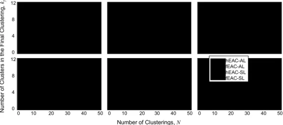
In this section we try to compare the performance of hEAC and fEAC for identifying the correct clusters when the clusters. Both single-linkage (SL) and average-linkage (AL) methods are used for cluster merging. For each ensemble, the final clustering is selected according to the maximum-lifetime criterion. In Fig. 2 we plot kf, the number

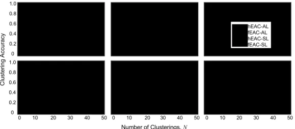
of clusters in the final clustering versus N, averaged over 20 ensembles. Results for both AL and SL are shown. In Fig. 2(e) and 2(f), the AL results are not visible because the numbers of clusters are more than 12. In addition, in order to validate the final clusterings, we also plot the clustering accuracy in Fig. 3. This is because just having the correct number of clusters (i.e., with kf equal to k*) does not necessarily imply a correct

clustering.

From Fig. 2 and Fig. 3, we can see that the best performer in each case, in terms of both accurate clustering results and fast convergence, is either fEAC-AL (for data sets S1-S3) or fEAC-SL (for data sets S4-S6). fEAC-SL is better for S4-S6, which contain well separated non-spherical clusters, and fEAC-AL is better for the touching clusters in S1 and S3. In all these cases, this best performer (fEAC-AL or fEAC-SL) is better than its crisp counterpart for N<10 and always converges to its optimal accuracy with smaller N. Fig. 4 is similar to Fig. 3 except that for each data set, we select the combined clusterings with the number of clusters equal to k*.

TABLEI Summary of Data Sets

Data Set Num. Patterns Num. Features k* _[k

min, kmax] Spherical-touching 500 2 5 [3, 12] Spherical-separated 500 2 5 [3, 12] Spherical-unbalanced 300 2 4 [3, 12] Cigar 200 2 4 [5, 20] Half rings 400 2 2 [20, 80] 3 rings 450 2 3 [20, 80] Iris 150 4 3 [2, 10] Breast cancer 683 9 2 [2, 10] Pen-digits 1000 16 10 [10, 50]

Figure 1. The 6 synthetic data sets used in our experiments. From left to right: spherical-touching (S1); spherical-separated (S2); spherical-unbalanced (S3); cigar (S4); half rings (S5); 3 rings (S6). Different colors represent the ground-truth cluster labels.

Other than generally better clustering accuracy compared to Fig. 3, which is no surprise, we can also clearly see faster convergence of the best-performing fEAC version relative to its hEAC counterpart.

For a more quantitative comparison regarding the dependence of the performance on N, let us now consider the value of N needed for the clustering accuracy to reach 95% of its maximum value in each case. For the 12 cases here (6 data sets with combined clustering selection based on maximum lifetime or known k*), the median N needed is 2 for the fuzzy versions and 11 for the corresponding crisp versions. It is evident then that fEAC converges much faster than hEAC with respect to N. Similar observation can be made for kf

when the maximum lifetime criterion is used. This is a clear indication that FCM is an attractive option for generating the base clusterings when the total number of base clusterings is constrained by, say, available system resource.

Fig. 5 displays the clustering performance (kf and accuracy

when using the maximum lifetime criterion, and accuracy when selecting the combined clustering with k* clusters) versus N for the three real data sets. The overall best performer is clearly fEAC-AL, although hEAC-AL is better

for the Pen-digits data set when using the maximum lifetime criterion. More importantly, faster convergence versus N for fEAC compared to hEAC is still evident here.

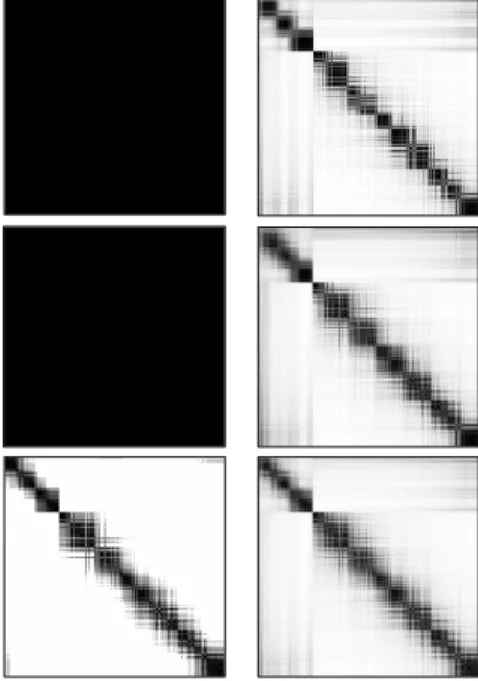
Overall, fEAC is better than hEAC when N is very small, and the main reason is because fEAC has much faster convergence. On the other hand, the performance of fEAC and hEAC for larger N is comparable for most cases. In order to provide insight to these observations, we show in Fig. 6 the co-association matrices of using hEAC (left column) and fEAC (right column) with three different N. The data set is half rings. We can see that while the co-association matrix becomes progressively fuzzier for hEAC as N increases, the co-association matrix for fEAC does not change much. The most significant difference here is between the co-association matrices between hEAC and fEAC at N=1. With only a single clustering, the co-association matrix is very crisp for hEAC but quite fuzzy already for fEAC. This directly results from the fact that with a clustering, HCM clusters are disjoint and FCM clusters overlap with one another. When N is large, the co-association matrices for hEAC and fEAC are more similar, as the "fuzziness" here is more of the result of averaging over many clusterings. Therefore, we can infer that the

0 10 20 30 40 50 0 10 20 30 40 50 0 10 20 30 40 50 12 8 4 0 Number of Clusterings, N N um ber of C lu s ter s i n the

(d) (e) hEAC-AL_fEAC-AL (f)

hEAC-SL fEAC-SL hEAC-AL fEAC-AL hEAC-SL fEAC-SL k* _{= 4 k}* _{= 2} k* _{= 3}

Figure 2. The number of clusters in the final clustering vs. the number of clusterings in each ensemble. (a)-(f) are plots for the synthetic data set S1-S6, respectively. The value of k* _{is also indicated in each plot.}

0 10 20 30 40 50 0 10 20 30 40 50 0 10 20 30 40 50 1.0 0.8 0.6 0.4 0.2 0 Number of Clusterings, N C lu s te ri n g Accu ra cy (a) (b) (c) (d) (e) (f) 1.0 0.8 0.6 0.4 0.2 0 hEAC-AL fEAC-AL hEAC-SL fEAC-SL hEAC-AL fEAC-AL hEAC-SL fEAC-SL

Figure 3. The clustering accuracy vs. the number of clusterings in each ensemble. The number of clusters in the final clustering is selected using the maximum-lifetime criterion. (a)-(f) are plots for the synthetic data set S1-S6, respectively.

overlapping between FCM clusters has an effect of "fuzzifying" the co-association matrix similar to averaging over several clusterings. The faster convergence of fEAC is then the result of similarly fuzzy co-association matrices at different N.

In addition to convergence speed, we are also interested in analyzing how the clustering performance is affected by noise. For this purpose, we add 40 randomly distributed noise points to each of the 6 synthetic data sets and re-do the experiments. It is expected that clustering accuracy will be degraded for the corresponding noiseless and noisy data sets. We are instead more interested in seeing how the performances of hEAC and fEAC are degraded differently. The plots for this purpose are in Fig. 7. Here the horizontal and vertical axes represent the

clustering accuracy difference between fEAC and hEAC for noiseless and noisy data sets, respectively. Each point corresponds to a combination of data set, SL/AL, N, and the two modes of combined clustering selection (maximum lifetime and pre-specified number of clusters). The majority of the points are above the diagonal, meaning that the degradation for fEAC due to the added noise points is less than that for hEAC. There, we can conclude that fEAC is more tolerant of noise than hEAC, even for large N values when both have converged for noiseless data.

V. CONCLUSIONS

In summary, we have presented in this paper experimental comparison between HCM and FCM as the base clustering

0 10 20 30 40 50 0 10 20 30 40 50 0 10 20 30 40 50 1.0 0.8 0.6 0.4 0.2 0 Number of Clusterings, N C lu s te ri n g A ccu ra cy (a) (b) (c) (d) (e) (f) 1.0 0.8 0.6 0.4 0.2 0 hEAC-AL fEAC-AL hEAC-SL fEAC-SL hEAC-AL fEAC-AL hEAC-SL fEAC-SL

Figure 4. The clustering accuracy vs. the number of clusterings in each ensemble. The number of clusters in the final clustering is set to be the same as k*_{. (a)-(f) are plots for the synthetic data set S1-S6, respectively.}

0 10 20 30 40 50 0 10 20 30 40 50 0 10 20 30 40 50 1.0 0.8 0.6 0.4 0.2 0 Number of Clusterings, N C lus te ri ng Ac c u ra cy (a) (b) (c) (d) (e) (f) 1.0 0.8 0.6 0.4 0.2 0 hEAC-AL fEAC-AL hEAC-SL fEAC-SL hEAC-AL fEAC-AL hEAC-SL fEAC-SL _{(g) (h) (i)} k* _{= 3 k}* _{= 2 k}* _{= 10} 20 15 10 5 0 kf

Figure 5. The clustering performance vs. N. for the three real-world data sets. (a)(d)(g) Iris; (b)(e)(f) Wisconsin breast cancer; (c)(f)(i) Pen-digits. (a)-(c) The number of clusters in the final clustering using the maximum lifetime criterion. (d)-(f) Clustering accuracy using the maximum lifetime criterion. (g)-(i) Clustering accuracy when the number of clusters in the final clustering is set to be the same as k*_.

clusterings is required for convergence. We also provide the insight into this observation by directly comparing the co-association matrices of hEAC and fEAC for different numbers of base clusterings. In addition, our experiments also show that fEAC is more tolerant of noise than hEAC.

There are still many research problems related to soft cluster ensembles that can be pursued. A more comprehensive study (such as one by varying the fuzzification factor) can lead to a more clear understanding of the phenomena associated with fuzzy cluster ensembles. Another direction is the use of non-probabilistic partitions (such as those obtained with possibilistic c-means [22] and its derivatives) as the base clusterings in the ensemble. Overall, we believe that the combination of fuzzy approaches and cluster ensembles will be of great values in future research and applications.

REFERENCES

[1] A.K. Jain, M.N. Murty, and P.J. Flynn, "Data Clustering: A Review", ACM Computing Surveys, vol. 31, pp. 264-323, 1999.

[2] S. Theodoridis and K. Koutroumbas, Pattern Recognition (3rd Ed.), San Diego, CA: Academic Press, 2006.

[3] A.K. Jain and M.H.C. Law, "Data clustering: A user’s dilemma", Lecture Notes on Computer Science, vol. 3776, pp. 1–10, 2005. [4] A. Strehl and J. Ghosh "Cluster ensembles -- a knowledge reuse

framework for combining multiple partitions", J. Machine Learning Research, vol. 3, pp. 583-617, 2002.

[5] A.L.N. Fred and A.K. Jain, "Combining multiple clusterings using evidence accumulation", IEEE Trans. Pattern Analysis Machine Intelligence, vol. 27, pp. 835-850, 2005.

[6] X.Z. Fern and C.E. Brodley, "Random projection for high dimensional clustering: A cluster ensemble approach", Proc. 20th Int'l Conf. Machine Learning (ICML), 2003.

[7] X.Z. Fern and C.E. Brodley, "Solving cluster ensemble problems by bipartite graph partitioning", Proc. 21th Int'l Conf. Machine Learning (ICML), ACM International Conference Proceeding Series, vol. 69, p. 36, 2004.

[8] A. Topchy, A.K. Jain, and W. Punch, "A mixture model for clustering ensembles", Proc. SIAM Int'l Conf. Data Mining, pp. 379-390, 2004. [9] A. Topchy, A.K. Jain, and W. Punch, "Clustering ensembles: Models of

consensus and weak partitions", IEEE Trans. Pattern Analysis Machine Intelligence, vol. 27, pp. 1866-1881, 2005.

[10] B. Minaei-Bidgoli, A. Topchy and W. F. Punch, “Ensembles of partitions via data resampling”, Proc. 2004 Int'l. Conf. Information Technology, pp. 188-192, 2004.

[11] K. Punera and J. Ghosh, "Soft Cluster Ensembles", in Advances in Fuzzy Clustering and its Applications, Ed. J. Valente de Oliveira and W. Pedrycz, Wiley, 2007.

[12] P. Viswanath and K. Jayasurya, "A fast and efficient ensemble clustering method", Proc. 2006 Int'l Conf. Pattern Recognition (ICPR), pp. 720-723, 2006.

[13] P. Hore, L. Hall, and D. Goldgof, "A Cluster Ensemble Framework for Large Data sets", Proc. 2006 IEEE Int'l. Conf. System, Man, and Cybernetics, pp. 3342-3347, 2006.

[14] R. Avogadri and G. Valentini , "Ensemble clustering with a fuzzy approach", Supervised and Unsupervised Ensemble Methods and their Applications, pp. 49-69, Springer, 2008.

[15] H. Luo, F. Kong, and Y. Li, "Clustering mixed data based on evidence accumulation", Lecture Notes on Computer Science, vol. 4093, pp. 348-355, 2006.

[16] J.C. Bezdek, Pattern Recognition with Fuzzy Objective Function Algorithms, New York: Plenum, 1981.

[17] L.I. Kuncheva and D.P. Vetrov, "Evaluation of stability of k-means cluster ensembles with respect to random initialization", IEEE Trans. Pattern Analysis and Machine Intelligence, vol. 28, pp. 1798-1808, 2006.

[18] Z. Yu, Z. Deng, H.-S. Wong, and X. Wang, "Fuzzy cluster ensemble and its application on 3D head model classification", Proc. 2008 IEEE Int'l Joint Conf. Neural Networks, (IJCNN), pp. 569-576, 2008. [19] J. Gllavata, E. Qeli, and B. Freisleben, "Detecting text in videos using

fuzzy clustering ensembles", Proc. 8th IEEE Int'l Symposium on Multimedia, pp. 283-290, 2006.

[20] L. Yang, H. Lv, and W. Wang, "Soft cluster ensemble based on fuzzy similarity measure", Proc. IMACS Multiconf Comp Eng Systems Appl, pp. 1994–1997, 2006.

[21] A. Asuncion and D.J. Newman, UCI Machine Learning Repository [http://www.ics.uci.edu/~mlearn/MLRepository.html]. Irvine, CA: University of California, School of Information and Computer Science, 2007.

[22] R. Krishnapuram and J.M. Keller, "A possibilistic approach to clustering", IEEE. Trans. Fuzzy Systems, vol. 1, pp. 98-110, 1993. 21ps03-vidmar

Figure 6. Co-association matrices (half-rings data set) at different N. Left and right columns are obtained using HCM and FCM, respectively. N = 1, 4, and 40 for the top, middle, and bottom row, respectively.

AL, mode A SL, mode A AL, mode B SL, mode B AL, mode A SL, mode A AL, mode B SL, mode B 0.6 0.4 0.2 0.0 -0.2 −0.2 0 0.2 0.4 0.6 −0.2 0 0.2 0.4 0.6

Clustering Accuracy Difference (Noiseless Data)

Cl us ter in g A c c u racy Di ff e renc e (N o isy D a ta ) N = 8 N = 20

Figure 7. Clustering accuracy difference (accuracy of fEAC minus accuracy of hEAC) with noiseless data (horizontal axis) vs. noisy data (vertical axis). Modes A and B refer to the use of maximum-lifetime criterion and the use of known k* for selecting the combined clustering, respectively.