Dimension Spectrum for Sofic Systems
JUNG-CHAO BAN∗†Department of Applied Mathematice National Dong Hwa University Hualien, 97401, Taiwan, R. O. C.
CHIH-HUNG CHANG, TING-JU CHEN AND MEI-SHAO LIN Department of Mathematics
National Central University Chung-Li, 32054, Taiwan, R. O. C.
September 10, 2010
Abstract
We study the dimension spectrum of sofic system with the potential is matrix-valued. For positive matrix and finite-coordinate dependent matrix potential, we set up the entropy spectrum by constructing the quasi-Bernoulli measure and the cut-off method is applied to deal with the infinite-coordinate dependent case. We extend this method to non-negative matrix and give a series of examples of the sofic-affine set on which we can compute the spectrum concretely.
Key words: Dimension spectrum, cut-off method, Gibbs-like measure, sofic system.
1
Introduction
Let (ΣA, T ) be a subshift of finite type (SFT) with A be the incidence matrix and T be its shift map. Motivated from the study of the iterated function systems (IFS) and generalized Sierpi´nski carpets (GSC, cf. [24, 21, 10, 11, 9]), one considers a special type of potential functions M : ΣA →
∗Ban is partially supported by the National Science Council, ROC (Contract No NSC
98-2628-M-259-001-), National Center for Theoretical Sciences (NCTS) and CMPT(Center for Mathematics and Theoretical Physics) in National Central University.
L(Rd, Rd) which take values on the set of d × d matrices. The study of the
thermodynamic properties with these potentials relates deeply to the fractal properties of the given IFS or GSC. Before formulating our results we recall some notations and background first. For q ∈ R, if M : ΣA→ L(Rd, Rd) is
infinite-coordinate dependent matrix-valued potential, define the topological pressure as follows: PM(q) = limn→∞n1 log X I∈ΣA,n sup x∈[I] ° ° °Qn−1l=0M (Tl(x)) ° ° °q, (1)
whenever the limit exists and ΣA,n denotes the collection of n-cylinders in
ΣA (Here kAk is the matrix norm, i.e., kAk = 11×dA1d×1 where 1d×1 is
the d × 1 column vector with entries are 10s). In [11], if M is positive, i.e., Mi,j > 0 and H¨older potential with ΣA is topologically mixing, the authors
prove that the Gibbs measure for M exists uniquely and the system admits the multifractal analysis. More precisely, they investigate the dimension spectrum for the upper Lyapunov exponent, i.e., for any α = PM0 (q), q 6= 0,
dimHEM(α) = log m1 {−αq + PM(q)} , (2)
where dimHA denotes the Hausdorff dimension of A and EM(α) is the level
set for the upper Lyapunov exponent EM(α) = x ∈ ΣA: limn→∞ log ° ° °Qn−1i=0 M (Ti(x))°°° n = α . (3)
We emphasize that the formula (2) set up the fine structure in the Hausdorff dimension point of view for (ΣA, T ). The authors extend this result to the
case that M is non-negative with some additional irreducible conditions, reader may refer to [10] for the detail. We mention here that the difficulty for non-negative M is that the product of matrix deeply effects the admissible words for the underlined space ΣA. For instance, let Σ = {0, 1, 2}Z be the full shift of 3 symbols, define the matrix-valued potential depends on one coordinate as M0 = · 0 1 0 1 ¸ , M1 = · 1 1 1 0 ¸ and M2 = · 0 0 1 1 ¸ , it can be checked that M0M1 ≥ 0 and M1M2 ≥ 0 and thus 01 and 12 are still
admissible words. However, M0M1M2 = 02×2, this makes 012 form a new
forbidden word of length 3 for Σ.
We note here, in [11], the existence of Gibbs measure is independent of the finite or infinite-coordinate dependent of the matrices M, they only
assume that M is H¨older. However, if M is only continuous and depends on infinite coordinates (cf. [9]). The dimension spectrum (2) still holds but altering to
dimHEM(α) = 1
log mq∈Rinf{−αq + PM(q)} (4)
since there may have more than two points attain the infimum of (4). We address here that in [9], the cut-off method is applied to create the new finite-coordinate dependent matrix potential, then a sequence of measures possesses the similar property of Gibbs (Lemma 4.3, [9]) can be constructed and all of them satisfy the quasi-Bernoulli property and formula (2). Finally the approximation method is applied to set up the formula (4).
In other direction, let S be a sofic shift which is a subshift of the shift space and S be the shift map on it. The well-known Curtis-Lyndon-Hedlund Theorem (Theorem 6.2.9, [20]) demonstrates that if φ : ΣA→ S is a func-tion, then φ is a homomorphism if and only if φ is a sliding block code. The sliding block code is induced from block map, i.e., a map Φ(L): Σ
A,L→ A(S)
for some L ≥ 1 and let π(L):= π
ZL be the restriction map of a cylinder to
ZL lattice. For all k ≥ 1 and if I ∈ Σ
A,k+L−1, define Φk : ΣA,k+L−1 → Sk
by Φk([I]) := Φ(L)(π(L)
¡
Tk−1([I])¢). Then φ : Σ
A → S is thus defined as
the limit of Φk, i.e., φ = limk→∞Φk and
S = {φ(x) : x ∈ ΣA} .
(We refer reader to [20] and [17] for more detail).
The thermodynamic properties with matrix potential and sofic space relate to fractal dynamics of a given sofic affine-invariant sets (cf. [16]). We formulate this setup for the convenience of our study. If T2= R2/Z2 which
is invariant under T = · n 0 0 m ¸
Let D = {0, . . . , n − 1} × {0, . . . , m − 1} and for any {dk}∞k=1 ∈ DN the base T representation is as follows: RT ({dk}) = ∞ X k=1 · n−k 0 0 m−k ¸ dk.
Let A be a matrix index by D be a incidence matrix and KT(A) is also defined as the image of RT, i.e.,
Let Φ(L): Σ
A,L→ D be defined by the block map and it induced an unique
directed graph, φ : ΣA→ D∞ is thus defined from the pair
¡
ΣA, Φ(L)
¢ and above formulation. The resulting system is called sofic system and we write S := φ (ΣA). One defines KT(n)(S) = {RT{dk} : (dk)k≥1∈ Sn= φ(ΣA,n+L−1)} and KT(S) = n RT {dk} : (dk)k≥1∈ S = φ (ΣA) o .
In [16], the authors extend the result of [21] to compute the dimension of KT(S).
Theorem 1 (Theorem 3.2, [16]) Let S be defined from φ : ΣA→ S and φ induced from ¡ΣA, Φ(L)
¢
for some L ≥ 2 with the incidence matrix A is primitive, then one can construct m matrices A0, A1, . . . , Am−1 which are indexed by D such that
dimHKT(S) = lim k→∞ 1 log m X I=(i0···in−1)∈ΣA,n ° ° °Qn−1k=0Aik ° ° °α where α = log m/ log n ≤ 1.
In this paper, we study the dimension spectrum with N : S → L(Rd, Rd)
is a matrix-valued potential on S taking values on the set of d × d matrices. To be precise, for q ∈ R, let PN(q) be defined similarly as in (1) and the level set for the upper Lyapunov exponent for N is also defined similarly as (3). EN(α) = J ∈ S : limn→∞ log ° ° °Qn−1l=0 N (Sl([J]))°°° n = α .
It can be proved that (Theorem 3) if N is finite-coordinate dependence, then if q 6= 0 and α = P0
N(q)
dimHEN(α) = 1
log λ{−αq + PN(q)} . (5)
Some remarks we address here is that the formula (5) help us to investigate the fine structure for a given sofic self-affine set. Secondly, our method is motivated by the cut-off method proposed by [9] and the intrinsic property of the sliding block code Φ(L) and φ, we formulate it briefly.
1. Since N depends on k coordinates, we construct Φkfrom Φ(L)as above.
Then the pull-back potential on ΣA,k+L−1 from Φk is also defined.
We extend the idea of the proof of Lemma 4.3 of [9] to construct an invariant, ergodic probability measure on ΣA,k+L−1 and extend this measure to some limiting measure which support on the whole ΣA.
2. For all J ∈ Snwe define a measure on J by measuring one of its
preim-age with the measure in ΣA which is constructed in Step1. Since the
measure in ΣA satisfies the Markov property and probability
proper-ties, then the measure on S can not share the same properties. How-ever, the space M(S) is still compact, the standard argument allows us to find an invariant and ergodic measure on S.
3. Combining step 1 and 2 we are able to show that the limiting measure is Gibbs-like and satisfies the quasi-Bernoulli property (We emphasize here that this measure is not necessary a Gibbs measure) and the Lq -spectrum preserved under the factor φ which is induced from the limit of lim
k→∞Φk. Therefore, the differentiability and the dimension spectrum
can be preserved from φ.
The block map Φ(L)plays an important role in this method and one of the
advantages of this method is that we can prove (2) holds for if N ∈ ΓH
+(S) by
using the matrix theory argument (Perron-Frobenius Theorem [18]). And this method also allows us to point out that the infimum of (4) can not be removed for some non-negative matrix potentials. To the best of our knowledge, this method is new and we will show there are some interesting examples of sofic affine set that we can compute their rigorous formula for Lq-spectrum and the pressure functions, then the dimension spectrum is
thus derived by simple computation.
To end this section we give an example as an application of this work to differential equations. Consider the one-dimensional multi-layer cellular neural networks (MCNN) as follows:
dx(n)i dt = −x (n) i + X |k|≤d a(n)k yi+k(n) + X |k|≤d b(n)k u(n)i+k+ z(n), for some d ∈ N, 1 ≤ n ≤ N ∈ N, i ∈ Z, where
u(n)i = yi(n−1) for 2 ≤ n ≤ N, u(1)i = ui, xi(0) = x0i
and
y = f (x) = 1
is the output function which is piecewise linear. A(n) = (a(n)−d, . . . , a(n)d ) is called the feedback template; B(n)= (b(n)
−d, . . . , b
(n)
d ) is called the controlling
template, z(n)is called the threshold. This equation comes from the coupling
of the the well-known CNN (cf. [6, 7, 8]) between the output solutions and it indicate the evolution of the effect for the neighborhood coupling. In [3], the authors investigate the complexity for the mosaic solutions for this MCNN and the analytical results shows that this solutions is no longer a SFT, but a strict sofic system. Some new phenomena appear is not analogous to the SFT case. The study the dynamics of these systems is more interesting and difficult than CNN and the above method for the dimension spectrum leads us to explore the inner structure for the distribution for the solutions of MCNN, this result appears in the forthcoming paper.
The content of the paper is following. In Section 2, we present the main result and its proof of this paper and give some examples. Since the dimension spectrum can also be derived from the differential of the pressure functions, the matrix H(k) defined in the main theorem allows us to deal
with the computation for the exact formula of the pressure functions and we provide this results in Section 3 and apply this result to some sofic self-affine sets.
2
Dimension spectrum
Let (ΣA, T ) be a subshift of finite type and φ : ΣA→ S be a sliding block code with Φ(L): Σ
A,L→ A (S) be its sliding block map. Denote by M(ΣA)
the set of probability measure on ΣAand MT(ΣA) the subset of T -invariant
measures of M(ΣA), M(S) and MS(S) are defined similarly. Let ΓF(+)(S) be the collection of d × d non-negative (positive) matrices which are F-continuous on S, notation F stands for the H of H¨older F-continuous or C for continuous, the same for ΓF(+)(ΣA). We call φ right-resolving if for all I1 = (i1;l)L−2l=0 and any I2 = (i2;l)L−2l=0 and I3 = (i3;l)L−2l=0 ∈ ΣA,L−1 such that I1⊕ I2 and I1⊕ I3 ∈ ΣA,L we have
Φ(L)([I1⊕ I2]) 6= Φ(L)([I1⊕ I3]),
where I1⊕ I2 = i1;0, i1;1, . . . , i2;L−2 ∈ ΣA,L if and only if i1;l+1 = i2;l ∀l =
0, . . . , L − 2. If I1, I2∈ A(ΣA), then I1⊕ I2:= I1I2. Throughout this paper
we assume φ : ΣA → S is right-resolving. We give some definitions for our study.
Definition 2 1. We say that µ ∈ MT(ΣA) is quasi-Bernoulli if there exists a constant C > 1 such that
C−1µ ([I1]) µ ([I2]) ≤ µ([I1I2]) ≤ Cµ ([I1]) µ ([I2]) ∀I1, I2 ∈
S
n∈N
ΣA,n. 2. For q ∈ R, the Lq-spectrum of µ is defined by
τµ(q) = log λ1 lim infn→∞ n1log
X
I∈ΣA,n
µ ([I])q where λ denotes the maximal eigenvalue of A.
The main result of the present paper is the following. Theorem 3 Let N ∈ ΓC
+(S) be a matrix-valued potential on S which
de-pends on k coordinates. Then
1. For all q ∈ R\ {0} , PN(q) is differentiable; 2. If α = P0
N(q),
dimHEN(α) = log λ1 {−αq + PN(q)} , (6) where λ is the maximal eigenvalue of A.
Proof. We divide the proof in the following 4 steps. Step 1. Let Φ(L) : Σ
A,L → A (S) be a sliding block code from ΣA,L to A (S) . For k ≥ 1, define Φk = Φ(k+L−1) from Σ
A,k+L−1 to Sk by Φk([I]) = J = (j0, · · · , jk−1), jl= Φ(L)(π[0,L−1] ³ Tl−1([I]) ´ ) ∀l = 1, · · · , k,
where π[0,L−1]([I]) = i0i1· · · iL−1 denotes the projection map to coordinate
[0, L − 1] on Z1 for all I ∈ ΣA. Define a matrix M on ΣA,k+L−1 by if I ∈ ΣA,k+L−1
M ([I]) = N (Φk([I])).
Then M is well-defined for all I ∈ ΣA,k+L−1from the fact that N depends on k-coordinate. Write Σ(k) = ΣA,k+L−1. Define q(k) = #ΣA,k+L−1 for k ≥ 1
and q(0) = #A(Σ
A), we setup a matrix H(k) ∈ Mdq(k−1)×dq(k−1) which is
indexed by the elements of Σ(k−1) as follows: ∀I
1, I2 ∈ Σ(k−1) HI1(k),I2 = M ([I1⊕ I2]) if I1⊕ I2 ∈ Σ(k) 0d×d otherwise. ,
where 0d×d denotes the d × d matrix with entries are all zeros. For all A = (Ai1,i2)ni1,i2=1 ∈ Mdn×dn(R) with Ai1,i2 ∈ Md×d(R), we denote by I(A)
the indicator matrix of A, i.e., I(A) ∈ Mn×n(R) I(A)i1,i2 = 1 if Ai1,i2 6= 0d×d 0 otherwise. .
It is obviously that if ΣA is mixing, then I(A) is primitive. Therefore, if
we assume H = H(k), there exists an uniform constant m > 0 such that for
all I1 and I2 ∈ Σ(k−1) there exists a path (I0
l)Rl=1 with R ≤ m, Il0 ∈ Σ(k−1), I0
1 = I1, IR0 = I2 and
I0:= I10 ⊕ · · · ⊕ IR0 ∈ Σ(k+R−2) Combining the fact of N ∈ ΓC
+(S) R−1Y l=0 M (π[0,k+L−2](Tl([I0]))) = R−1Y l=0 N (Φk◦ π[0,k+L−2](Tl¡[I0]¢)) > 0. Thus HI1,I2R ≥ R−1Y l=1 M (π[0,k+L−2](Tl([I0]))) > 0,
and also Hm > 0. Let A(k) = ©I(l)∈ Σ(k−1) : l = 1, . . . , q(k−1)ª be an
or-dered set by the lexigraphic ordering and we rearrange H according to this ordering. Since H is primitive, Perron-Frobenius Theorem is applied to show that there exist eigenvalues ρLand ρR> 0 with corresponding eigenvectors L and R > 0 respectively for H. We may also assume
That is,
(LH) ([I(l)]) = X
I(j)∈Σ(k−1): I(j)⊕I(l)∈Σ(k)
L([I(j)])M ([I(j)⊕ I(l)]) = ρLL([I(l)]) (7)
(HR) ([I(l)]) = X
I(j)∈Σ(k−1): I(l)⊕I(j)∈Σ(k)
M ([I(l)⊕ I(j)])R([I(j)]) = ρRR([I(l)]). (8)
For all I ∈ Σ(k+j) and j ≥ 0, let π(k)= π
[0,k+L−2]and Q [I]M = "j−1 Y l=0 M (π(k)(Tl([I]))) # , we define a measure as follows.
ηL([I]) = ρ−jL L(π(k−1)([I]))hQ[I]M i R(π(k−1)¡Tj−1([I])¢), (9) ηR([I]) = ρ−jR L(π(k−1)([I])) hQ [I]M i R(π(k−1)¡Tj−1([I])¢). It follows from (7) and (8) that if I ∈ Σ(k+j−1)
X I1∈Σ(k−1): I1⊕I∈Σ(k+j) ηL([I1⊕ I]) = X I1∈Σ(k−1): I1⊕I∈Σ(k+j)
ρ−jL L(π(k−1)([I1⊕ I]))hQ[I1⊕I]M i R(π(k−1)¡Tj−1([I1⊕ I])¢) = ρ−(j−1)L L(π(k−1)(T ([I])))hQ[I]M i R(π(k−1)(Tj−1([I]))) = ηL([I]). That is, X I1∈Σ(k−1): I1⊕I∈Σ(k+j)
ηL([I1⊕ I]) = ηL([I]).
It follows from the same computation we also have ηR([I]) =
X
I1∈Σ(k−1): I⊕I1∈Σ(k+j)
This implies that ∀n ≥ 0, X I∈Σ(k+n) ηL([I]) = X I∈Σ(k) ηL([I]) and X I∈Σ(k+n) ηR([I]) = X I∈Σ(k) ηR([I]).
It can be easily checked that ρL= ρR and then we define η([I]) = ηLη(k)−1, where η(k)=
X
I∈Σ(k)
ηL([I]).
The Kolmogorov consistence theorem applies to show that there exists a measure µ on ΣA such that
µ([I]) = η ([I]) ∀I ∈ ∪n≥0Σ(k+n).
Step 2. In this step, we will define a measure on MS(S). Since Φk+j
³ Σ(k+j)
´
= Sk+j
is onto, for all J ∈ Sk+j we define an ordered set PJ :=
n
I(l)∈ Σ(k+j): Φk+j([I(l)]) = J
o . and set a measure on S
ξ1([J]) = ηL([I(1)]), ∀J ∈ Sk+j, I(1) ∈ PJ. We note here that ξ1 is not invariant. Let
ξ([J]) = ξ1([J]) ξ(k)−1 where ξ(k)=
X
J∈Sk
ξ1([J]).
For all J ∈ Sk+j and assume I1, I2 ∈ PJ ∩ Σ(k+j),
Φk(π(k)(Tl([I1]))) = Φk(π(k)(Tl([I2]))) ∀l = 0, · · · , j − 1. Hence j−1Y l=0 M (π(k)(Tl([I1]))) = j−1 Y l=0 N (Φk(π(k)(Tl([I1])))) (10) = j−1 Y l=0 N (Φk(π(k)(Tl([I2])))) = j−1 Y l=0 M (π(k)(Tl([I2]))).
Set
UL= max
i=1,··· ,dI∈Σmax(k−1)Li([I]) and UR= maxi=1,··· ,dI∈Σmax(k−1)Ri([I]), VL= min
i=1,··· ,dI∈Σmin(k−1)Li([I]) and VR= mini=1,··· ,dI∈Σmin(k−1)Ri([I]),
where Di([I]) denotes the i-coordinate of vector of D([I]) for D = L or R. Since φ = limk→∞Φk is right-resolving, for all J ∈ Sn there is at least one
and at most K preimages of I ∈ Σ(n) such that Φ
n([I]) = J. Therefore, if j ≥ 0 and J ∈ Sk+j it follows from (10)
ρ−jVLVR ° ° ° ° ° j−1Y l=0 M (π(k)(Tl([I]))) ° ° ° ° ° ≤ ηL([I]) ≤ ηL ³ Φ−1k+j([J]) ´ = ηL Ã S I∈PJ∩Σ(k+j) [I] ! ≤ X I∈PJ ηL([I]) ≤ ρ−jKULUR ° ° ° ° ° j−1Y l=0 M (π(k)(Tl([I]))) ° ° ° ° °.
It also follows from the positivity of L = (L(I(l)))q(k−1)
l=1 , R = (R(I(l)))q (k−1) l=1
and q(k−1) is finite. We can conclude that there exist two constants P and
Q > 0 such that 1 ≤ UL/VL≤ P and 1 ≤ UR/VR≤ Q then ηL ³ Φ−1k+j([J]) ´ ≤ ρ−jKULUR ° ° ° ° ° j−1 Y l=0 M (π(k)(Tl([I]))) ° ° ° ° ° ≤ KP QVLVR ° ° ° ° ° j−1Y l=0 M (π(k)(Tl([I]))) ° ° ° ° ° ≤ KP QL(π(k−1)([I])) j−1Y l=0 M (π(k)(Tl([I])))R ³ π(k−1)(Tj−1([I])) ´ = KP Qξ1([J]). and ηL ³ Φ−1k+j([J]) ´ ≥ VLVR ° ° ° ° ° j−1 Y l=0 M (π(k)(Tl([I]))) ° ° ° ° °≥ P −1Q−1ξ 1([J]) .
This means that for all J ∈ Sk there exists a constant C1 > 0 such that
C1−1ξ1([J]) ≤ ηL
¡
and thus
C2−1ξ([J]) ≤ η¡Φ−1k ([J])¢≤ C2ξ([J]),
for some C2 > 0.
Step 3. Since ξ is not invariant, we follow the proof of [11] to construct an invariant and ergodic measure satisfies the property of (9) in this step. For all J ∈ Sk, defining a sequence
nPn−1 l=0 ξ ◦ S−l([J]) o n≥1. It follows from (11) that if l ≥ 0 ξ1◦ S−l([J]) = X J1J∈Sl+k ξ1([J1J]) = X I1I∈PJ1J∩Σ(l+k) ηL([I1I]) ≤ X I1I∈PJ1J∩Σ(l+k) ηL ¡ Φ−1([J1J]) ¢ ≤ C3ηL([I])
for some constant C3 > 0. Thus there exists a C4 > 0 such that C4−1η¡Φ−1k ([J])¢≤ ξ ◦ S−l([J]) ≤ C4η
¡
Φ−1k ([J])¢ Since S is compact, then let ν ∈ M(S) be the limiting measure of
(n−1 X l=0 ξ ◦ T−l([J]) ) n≥1 .
Combining the fact that limn→∞Φk+n= φ with above computations yields ν ¿ µ and µ ¿ ν. Up to a small modification of the proof in Theorem 1.1 of [11] we also have that ν is ergodic. The Radon-Nikodym theorem applies to show that there is a constant C > 0 such that ν ([J]) = Cµ¡Φ−1l ([J])¢ for ν-a.e. J ∈ Sl and l ≥ k. It follows from that ν and µ are both invariant
probability measures we obtain C = 1 and for all J ∈ S ν([J]) = lim
l→∞µ
¡
Φ−1l ([J])¢= µ(φ([J])).
Step 4. From the above computation we obtain that there exists Q > 0 such that if J ∈ Sl with l ≥ k and I(1) ∈ PJ
Q−1ρ−jL L(π(k−1)([I(1)]))hQ[I(1)]M i R(π(k−1)(Tj−1([I(1)]))) ≤ ν([J]) = µ([I(1)]) ≤ Qρ−jL L(π(k−1)([I(1)]))hQ[I(1)]M i R(π(k−1)(Tj−1([I(1)])))
Hence ν ∈ MS(S) is a quasi-Bernoulli measure. According to the fact that right-resolving factor φ cannot increase the topological entropy we can assert that
τν(q) = τφ∗µ(q) = τµ(q) for any q ∈ R,
where φ∗µ = µ(φ−1). Theorem 1.3 of [11] is applied to show that for all q ∈ R\ {0} , τν is differentiable and if α = PN0 (q)
dimHEN(α) = 1
log λ(−αq + PN(q)) ,
where λ denotes the maximal eigenvalue of A. Finally, the differentiability for PN(q) with q 6= 0 comes from the fact PN(q) = PM(q) since φ is
right-resolving and M is the push-back potential of N. This completes the proof.
Remark 4 We remark that in the proof of Theorem 3, ν ∈ MS(S) is not a Gibbs measure, and in the following, we will show that this method allow us to approximate the potential depends on ∞-coordinate for N ∈ ΓH
+.
The idea of Theorem 3 leads to the study of the dimension spectrum for non-negative N . Before formulating our results we give the definition of a non-singular matrix first.
Definition 5 We call A ∈ Mn×n(R) non-singular if for all 1 ≤ j ≤ n we have Pni=1Aij ≥ 1. We also denote by Nn the collection of non-singular matrices of size n × n.
It can be easily verified that Nnforms a semi-group under matrix prod-uct.
Lemma 6 If A and B ∈ Nn then AB ∈ Nn.
Proof. Indeed, for all j = 1, · · · , n
n X i=1 (AB)ij = n X i=1 n X k=1 AikBkj = n X k=1 Bkj à n X i=1 Aik ! ≥ n X k=1 Bkj ≥ 1.
This completes the proof.
For non-negative matrix-valued potential N , we have the following result. Corollary 7 Let N ∈ ΓH(S) ∩ N
d depends on k-coordinate and there exists a finite set Λ ⊂ S
n≥k
Σ(n)=: Σ∗ such that for all I
1 and I2 ∈ Σ∗ there exists
I ∈ Λ such that I1⊕ I ⊕ I2 ∈ Σ∗ and M(k)([I]) = N (Φk([I])) > 0 for all I ∈ Λ, then (6) holds.
Proof. We give the proof for the case that all elements in Λ are equal length and the case for different length is in the same fashion. It follows from the proof in Theorem 3 that H(k)can be construct which is indexed by the Σ(k).
Since for any ω ∈ Λ, |ω| = k + L − 1 (we assume that Λ is equal length and from the definition Λ ⊂ Sn≥kΣ(n) it allows us to define all elements have
equal length of k + L − 1) we also assume that Λ consist only one element, say I∗. Without loss of generality, assuming I∗ ∈ Σ(k−1). It suffices to show
that H(k) is primitive. Indeed, for any I
1 and I2 ∈ Σ(k−1), since N ∈ Nd ,
Lemma 6 is thus applied to show that
HI1,I22 = M ([I1⊕ I∗])M ([I∗⊕ I2]) = N (Φk([I1⊕ I∗]))N (Φk([I∗⊕ I2])) > 0. This means that H2 > 0. The other case can be done similarly. Therefore,
the same proof as in Theorem 3 leads (6) and the proof is completed. In the proof of Theorem 3, the Lq-spectrum plays an important role for
the dimension spectrum. We emphasize that for a measure µ ∈ MT(ΣA) it is not easy to compute the rigorous formula for τµ. If the measure µ
as in Theorem 3, the following theorem provides a class of matrix-valued potentials for which we can compute its Lq-spectrum explicitly. Let N ∈
ΓH(S) ∩ Nddepends on k-coordinate and H := H(k) as defined in Theorem
3, we define a matrix R(q) ∈ Mq(k−1)×q(k−1) from H (recall that q(k) =
#ΣA,k+L−1) as follows: R(q)I1,I2 =
½
ρ(M ([I1⊕ I2]))q, if I1⊕ I2∈ Σ(k);
0, otherwise.
ρ (A) ∈ R denotes the maximal eigenvalue of A ∈ Md×d(R).
Theorem 8 Under the same assumptions of Corollary 7 and assume that N = {N ([J])}J∈Sk ∈ ΓH(S)
satisfies that
N ([J1])N ([J2]) = N ([J2])N ([J1]) for all J16= J2∈ Sk.
That is, N = {N ([J])}J∈Sk are simultaneously diagonalizable. Assume that H(k) and ν ∈ M
S(S) are as defined in Theorem 3. Then τν(q) = log λ1 (−q log ρ + log Θ(q)) ,
where Θ(q) is the maximal root of the characteristic polynomial of R(q) ∈ Mq(k−1)×q(k−1).
Proof. Let
H = [M ([I1⊕ I2])]I1,I2∈Σ(k−1)
be constructed as in the Step 1 of the proof of Theorem 3. Since elements of N are mutually commuted, then the set of matrices {M ([I])}I∈Σ(k) can be
diagonalized simultaneously. That is, there exists a unique P ∈ Md×d(R)
such that P M ([I])P−1 is a diagonal matrix for all I ∈ Σ(k). Since H is
primitive, there exists L and R > 0 such that (7) and (8) hold. We first compute the Lq-spectrum τ
µ, where µ ∈ MT(ΣA) is defined in the proof of
Theorem 3.
τµ(q) = log λ1 n→∞lim n1log
X I∈ΣA,n µ([I])q = 1 log λ −q log ρ + lim n→∞ 1 nlog X I∈ΣA,n ° ° ° ° ° n−1Y l=0 M (π(k)(Tl([I]))) ° ° ° ° ° q = 1 log λ −q log ρ + lim n→∞ 1 nlog X I∈ΣA,n P n−1Y l=0 ρ ³ M (π(k)(Tl([I]))) ´q P−1 = 1 log λ −q log ρ + lim n→∞ 1 nlog X I∈ΣA,n n−1Y l=0 ρ ³ M (π(k)(Tl([I]))) ´q = 1 log λ(−q log ρ + Θ(q)) .
We note here the second equality comes from the positivity of L, R and P is invertible. Since τν(q) = τµ(q) = τφ∗µ(q). The proof is completed.
Here we give a concrete example for the dimension spectrum of sofic system.
Example 9 Let ΣA be the golden mean shift with A = · 1 1 1 0 ¸
and the right-resolving sliding block code with L = 2
Φ(2)([00]) = a, Φ(2)([01]) = b and Φ(2)([10]) = b. Define a matrix potential on S1, i.e., k = 1 as in Theorem 8 by
Na= · 1 1 1 1 ¸ and Nb = · 1 0 0 1 ¸ .
Then Λ = {[00]} and M ([00]) = Na> 0. Theorem 3 indicates that PN(q) is differentiable. If α = P0
N(q) with q 6= 0, Corollary 7 is applied to show that
dimHEN(α) = −αq + PN(q). On the other hand, one can easily compute that
R(q) = ·
2q 1q
1q 0 ¸
and Theorem 8 applies to show that τν(q) = log g1 (−q log ³ 1 +√2 ´ +2 q+√22q+ 4 2 ), where g = 1 +√5 2 .
Theorem 3 deals with the finite-coordinate dependent matrix potentials. The cut-off method allows us to set up the dimension spectrum for infinite-coordinate dependent one for S. We emphasize here that our method makes the discussion of the limiting measure on infinite-coordinate systems possi-ble. Let ηk := sup ½ Mi,j(x) Mi,j(y) : I ∈ ΣA,n, x, y ∈ [I] , 1 ≤ i, j ≤ d ¾ .
Since M ∈ ΓH+(ΣA), we have |log ηn| ≤ Cλ−αn for some 0 < α < 1
(Lemma 2.2, [11]). The following result deals with the dimension spectrum for infinite-coordinate N .
Theorem 10 Let N ∈ ΓH
+(S) be a matrix-valued potential on S which
1. Define N(k)([J]) = max
y∈[J]N (y) for k ∈ N, J ∈ Sk. Then there exists ν(k)∈ M
S(S) such that PN(k)(q) is differentiable. Furthermore, if α = PN0 (k)(q), we have
dimHEN(k)(α) =
1
log λ{−αq + PN(k)(q)} . 2. The limit of ν(k) exists, i.e.,
lim
k→∞ν
(k)= ˜ν in the weak-star topology.
Furthermore,
dimHEN(α) = 1
log λ{−αq + PN(q)} . (12) Proof. The first statement is an immediate consequence of Theorem 3 since N(k) depends on k-coordinate. It remains to prove the second statement.
For k ≥ 1, I ∈ Σ(k) with I ∈ P
J, let H(k)∈ Mdq(k−1)×dq(k−1)(R) and ρ(k)
be its maximal eigenvalues as in Theorem 3. Since I(H(k)) is primitive and M(k)is positive, H(k)is also primitive for all k ∈ N. We claim that η−1
k ρ(k)≤ ρ(k+1)≤ η
kρ(k)for k ≥ 1. Indeed, let H(k)and H(k+1)be indexed by Σ(k−1)
and Σ(k) respectively. For all I ∈ Σ(k+1), [J] = [j0. . . jk] := Φk+1([I]), M(k+1)([I]) = N(k+1)(Φk+1([I])) = max
y∈[j0···jk] N (y) ≤ ηk max y∈[j0j1···jk−1] N (y) = ηkN(k)([J∗]) = ηkM(k)([I∗]) , where J∗:= j
0· · · jk−1 and I∗ := i0· · · ik+L−1. Therefore, for m ≥ 1,
° ° °H(k+1)m ° ° ° = X I∈Σ(k+m) ° ° ° ° ° m−1Y l=0 M(k+1)(π(k+1)(Tl([I]))) ° ° ° ° ° ≤ (ηk)m X I∈Σ(k+m) ° ° ° ° ° m−1Y l=0 M(k)(π(k)(Tl([I]))) ° ° ° ° ° ≤ C (ηk)m X I∈Σ(k+m−1) ° ° ° ° ° m−1Y l=0 M(k)(π(k)(Tl([I]))) ° ° ° ° ° = C (ηk)m ° ° °H(k)m ° ° ° ,
for some C > 1. Hence°°H(k+1)m°°m1 ≤ Cm1 (η k) ° °H(k)m°°m1 . Taking m → ∞ we have ρ(k+1)≤ ηkρ(k), for k ≥ 1.
Using the same argument we also have
ρ(k+1)≥ ηk−1ρ(k), for k ≥ 1. (13) On the other hand, for I ∈ Σ(k+j)with j ≥ 1 is fixed,
µ(k+1)([I]) = (ρ(k+1))−(j−1)L(k)(π(k+1)([I]))³Y[I]M(k+1) ´ R(k)(π(k+1)(Tj−2([I]))) ≤ D × (ρ(k+1))−(j−1) ° ° °Y[I]M(k+1) ° ° ° ≤ D × (ρ(k))−(j−1)ηj−1k ° ° °Y[I]M(k+1) ° ° ° (By(13)) ≤ D0× (ρ(k))−(j−1)ηkj−1ηj−1k ° ° °Y[I]M(k) ° ° ° ≤ D00ηk2j−2µ(k)([I]),
for some D, D0, D00 > 0. Similarly we have
µ(k+1)([I]) ≥ (D00ηk2j−2)−1µ(k)([I]).
The fact that limk→∞ηk = 1 asserts there exists D1 > 0, n ∈ N such that
for k ≥ n we have
D−11 µ(k)([I]) ≤ µ(k+1)([I]) ≤ D1µ(k)([I]).
This demonstrates µ(k) → ˜µ as k → ∞ for some ˜µ. Define ˜ν = φ∗µ.˜ ν(k)= φ ∗µ(k) implies lim k→∞ν (k) = lim k→∞φ∗µ (k)= φ ∗µ = ˜˜ ν.
It can also be checked that ˜µ satisfies the quasi-Bernoulli property and for all q ∈ R\ {0},
τµ˜(q) = lim
k→∞τµ(k)(q).
Using the same proof of Theorem 3, we have τµ˜(q) = lim
k→∞τµ(k)(q) = limk→∞τφ∗µ(k)(q) = limk→∞τν(k)(q) = τν˜(q),
and the desired equality (12) follows. This completes the proof.
We extend the result of Theorem 3 to non-negative matrix N which depends on finite coordinates.
Theorem 11 Let N ∈ ΓH(S) be a matrix-valued potential on S which de-pends on k coordinates. Then for all q ∈ R\ {0} and α = P0
N(q)
dimHEN(α) = log λ1 inf {−αq + PN(q)} .
Proof. For all I ∈ Σ(k), put Mε([I]) = M ([I]) + ε1
d×d, where 1d×d is
the full matrix of size d × d. By Theorem 3 there exists µε ∈ M T(ΣA)
and νε ∈ MS(S) with φ∗µε = νε. Since H 7→ ρ(H) is continuous, H is
irreducible and ρε is bounded, there exists a convergent subsequence ρεn
such that limn→∞ρεn = ρ∗ for some ρ∗. According to N ∈ Nd we have for
all I ∈ Σ(k+j), µεn([I]) = (ρεn)−jLεn(π(k−1)([I]))hQ [I]Mεn i Rεn(π(k−1)¡Tj−1([I])¢), where Q [I]Mεn = "j−1 Y l=0 Mεn(π(k)(Tl([I]))) # .
The same argument as Theorem 3 shows that we have limn→∞µεn = µ is
also quasi-Bernoulli and the it admits Lq-spectrum then the result follows.
This completes the proof.
To end this section we give some remarks for the convergence of the µε
in the proof of Theorem 11 for non-negative matrix.
Remark 12 1. Readers may wonder why we do not define the measure on H directly. The reason is that according to the Perron-Frobenius Theorem, there are more than one eigenvalues on the complex plane whose norm attain the maximal of the spectral radius of H, this makes the measure not well-defined.
2. As in Theorem 10, for the case of N ∈ ΓH+(S), we do prove that the limit of ρ(k) exists and this coincides with the unique simple
max-imal eigenvalue of H. However, in Theorem 11, although Mε > 0 the limε→0Mε may have more than 1 maximal eigenvalues. And the number of those maximal eigenvalues depends on the periodicity of the matrix H (cf. [17, 14]). Thus one can construct an example that the limit of µε is not convergent.
3. It is of interest to know whether the results of Theorem 7, Theorem 8 and Theorem 12 hold for q → ∞. And it is worth pointing out that this
topic is related to the study for the existence of ground states at tem-perature zero([5, 26, 25, 12, 22, 4, 15, 19, 13]). To be precise, let νqbe the unique measure at q ∈ R\ {0} , does this sequence {νq}q>0 conver-gent? If it is not the case, nature question arise: how to characterize the number and shapes of these convergent subsequences? The recent work ([2]) presents that if S is a sofic system induced by (ΣA, Φ(L)) for some L > 0 and ΣAis a SFT with N ∈ ΓH
+(S), then there are only
finite subsequence of {νq}q>0 on S. And if N ∈ ΓH(S), it is surpris-ing to show that there are infinite convergent subsequences. We also extend these results to countable system in the forthcoming paper ([1]).
3
Dimension spectrum via the pressure
Let (ΣA, T ) be a subshift of finite type and PM(q) be its pressure for q ∈
R. If PM(q) is differentiable, Theorem 1.3 of [11] demonstrates that the dimension spectrum can be computed via the formula of PM(q). However,
the computation of the explicit formula for PM(q) is not easy. If (S, S) be a
sofic system, we provide a wide class of matrix potential on S for which we can compute its PN(q) rigorously which leads to the dimension spectrum of EN(α). We first give a theorem which is analogous to Theorem 1.3 of [11].
Theorem 13 Let N ∈ ΓH
+(S). We have for any α = PN0 (q) with q 6= 0,
dimHEN(α) = log λ1 (−αq + PN(q)). (14)
Proof. Up to a minor modification, the proof is identical to the proof of Theorem 1.3 of [11] and we omit here.
We prove the following class for which we can compute its PN(q) and
dimHEN(α).
Theorem 14 If N ∈ ΓC(S) depends on k-coordinate satisfies the following properties
1. Let H = H(k) be the matrix constructed in Theorem 3 which is
primi-tive.
2. Let M ∈ ΓC(Σ(k)
A ) be induced from N , there exists a sequence χ =
(χI)I∈Σ(k)
A
and K ∈ M1×d(R) is a row vector such that for any I ∈ Σ(k)A we have
Then
PN(q) = log Θ(q),
where Θ(q) denote the maximal eigenvalue of F(q) ∈ Mq(k−1)×q(k−1)(R) de-fined in (16) and thus differentiable. Furthermore, (14) can be computed explicitly. Proof. Define F(q) ∈ Mq(k−1)×q(k−1)(R) by F(q)I1,I2 = ½ (KM ([I1⊕ I2])Y )q, if I1⊕ I2 ∈ Σ(k); 0, otherwise. (16)
where Y ∈ Md×1(R) is a column vector with KY = 1. Since H is primitive, then the left and right eigenvectors are positive, i.e., L, R > 0. Combining (15) with Perron-Frobenius Theorem we have
PN(q) = limn→∞n1 log X J∈Sn sup y∈[J] °
°N(y)N(S (y)) · · · N(Sn−1(y))°°q
= lim n→∞ 1 nlog X J∈Sn °
°N(y)N(S (y)) · · · N(Sn−1(y))°°q
= lim n→∞ 1 nlog X I∈Σ(n):
Φn([I])=J, x∈I and φ(x)=y
° °M(x)M(T (x)) · · · M(Tn−1(x))°°q = lim n→∞ 1 nlog X I∈ΣA,n+L−1 ° ° ° ° ° n−1Y l=0 M (π(k)(Tl(Φk) [I])))) ° ° ° ° ° q = lim n→∞ 1 nlog X I∈ΣA,n+L−1 ¡ χΦk([I])· · · χΦk(Tn−1([I])) ¢q (By (16)) = log Θ(q)
The second equality is because N is finite-coordinate dependent and 4th
equality comes from the right-resolving property of φ. This completes the proof.
Remark 15 1. In Theorem 3, we always assume that if one regards as ΣA= (G, E) where G = © I : I ∈ Σ(k−1)ªand edges E = n (I1, I2) : I1⊕ I2∈ Σ(k) o .
Then there only one level from I1 to I2 ∈ Σ(k), i.e., the number of
constructed with the entry is a single small matrix. However, if there are more than one levels from I1 to I2, since φ is right-resolving, then
we only need to add other small matrices in the entry of HI1,I2(k) , i.e.,
HI1,I2(k) = l (I1⊕ I2) M ([I1⊕ I2]) if I1⊕ I2∈ Σ(k) 0d×d otherwise. ,
where l (I1⊕ I2) denotes the number of levels from I1 to I2 and Theo-rem 3 still follows.
2. In the assumption (15) of Theorem 14, one can easily check that the result remains if there exists a column vector K such that for any I ∈ Σ(k)A
M ([I])K = χIK.
3. One can also easily checked that for those class of Theorem 14, if ν ∈ MS(S) is the measure in Theorem 3, Then the Lq-spectrum of
τν(q) = log λ1 (−q log ρ + log Θ(q)) ,
where ρ is the maximal eigenvalue of H(k) and Θ(q) is the maximal
eigenvalue of (16).
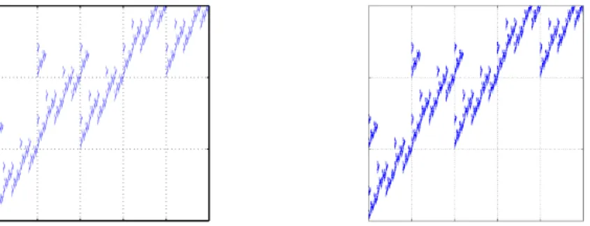
Example 16 (Example 1 of [23]) Let S be a sofic system of 3 symbols, say {0, 1, 2}, with substitution rules as in Figure 1, and N = (N ([s]))2s=0 be defined as N ([0]) = · 1 0 1 2 ¸ , N ([1]) = · 2 1 0 1 ¸ and N ([2]) = · 2 2 0 0 ¸ . KT(4)(S) and KT(7)(S) are represented in Figure 2. Define Φ(2) by
Φ(2)([00]) = Φ(2)([30]) = Φ(2)([40]) = [0],
Φ(2)([01]) = Φ(2)([11]) = Φ(2)([21]) = [1], Φ(2)([i2]) = [2] for 1 ≤ i ≤ 4. Then one can easily checked that if K = (1, 1) then χ = (χI)I∈Σ2 can be defined as
(0,0) (4,0) (3,0) (0,1) (0,0) (4,2) (2,1) (3,2) (1,1) (0,1) (1,2) (2,2)
a
b
a
a
a a
a a
a
b
b
b b
b
b b
Figure 1: The substitution rules associated with KT. H(1) can be defined as follows ((1) of Remark 15),
H(1)= · N ([0]) + 2N ([1]) + 2N ([2]) N ([1]) + 2N ([2]) N ([0]) 2N ([0]) + N ([1]) ¸ . For any q ∈ R, define F(q) from H by taking K = (1, 1) and Y =
µ 3 4 1 4 ¶ F(q) = · 5 × 2q 3 × 2q 1 × 2q 3 × 2q ¸ , Then
PN(q) = log Θ(q) = log 6 + q log 2.
If N is symmetric we also have the following estimation.
Corollary 17 Let N ∈ ΓC(S) depends on k-coordinate and H = H(k) be
the matrix constructed in Theorem 3 which is primitive. Let M ∈ ΓC(Σ(k) A ) be induced from N , if for any I ∈ Σ(k)A , there exist aI, bI ∈ R such that
M ([I]) = · aI bI bI aI ¸ .
Figure 2: The first and second figures are forth and seventh steps of iteration, respectively.
Then
PN(q) = log Θ(q),
where Θ(q) denote the maximal eigenvalue of F(q) ∈ Mq(k−1)×q(k−1)(R) which is defined by F(q)I1,I2 = (aI+ bI)q if I := I1⊕ I2 ∈ Σ(k) 0 otherwise. . (17)
Proof. Since for any I ∈ Σ(k)A , [1 1] · aI bI bI aI ¸ = (aI+ bI) · 1 1 ¸ .
Then Theorem 14 is applied to show that PN(q) = log Θ(q) where Θ(q) is the maximal eigenvalue of (17). The proof is completed.
Example 18 (Continued) Under the same substitution rule of Example 16, if the potential on S1 are as follows
N ([0]) = · 2 1 1 2 ¸ , N ([1]) = · 1 3 3 1 ¸ and N ([2]) = · 0 1 1 0 ¸ . One can easily checked that H(1) is primitive and define
F(q) = · 3q+ 2 × 4q+ 2 × 1q 4q+ 2 × 1q 3q 2 × 3q+ 4q ¸ . (18)
Then
PN(q) = log Θ(q), where Θ(q) denotes the maximal eigenvalue of (18).
To end this section, we give a result which extends Theorem 14 to infinite-coordinate dependent N .
Let N ∈ ΓH
+(S). Assume that #A(S) = s. For each k ≤ l ∈ N and
J ∈ Sl, define
N(l)([J]) = max
y∈[J]N (y).
Then N(l) ∈ ΓC
+(S). Let M(l) be induced by N(l), we say N satisfies
condi-tion (H) if
(i) For each l ∈ N there exists K(l) such that
K(l)M(l)([I]) = χ(l)I K(l);
(ii) For any I ∈ Σ(l)A and l ≥ k, there exists δ1, . . . , δs> 0 such that χ(l+1)Ij = δjχ(l)I for all j = 1, . . . , s,
where Ij ∈ Σ(k+1)A
For l ≥ k, let H(l) ∈ Mdq(l−1)×dq(l−1)(R) be constructed as in Theorem
3 indexed by the set of ΣA,l+L−1 and F(l)(q) ∈ Mq(l−1)×q(l−1)(R) be defined
similarly as (16). Denote by Θ(l)(q) the maximal eigenvalue of F(l)(q).
In the following we extend Theorem 14 to infinite-coordinate dependent matrix-valued potential.
Theorem 19 If N ∈ ΓC
+(S) satisfies condition (H) with 0 ≤ δj < 1 for all j = 1, . . . , s. Then PN(q) is differentiable and
PN(q) = lim
l→∞log Θ
(l)(q).
Proof. The proof is an immediate consequence of combining Theorem 10 and Theorem 14, we omit here.
References
[1] J.-C. Ban and W. Huang. Zero temperature limit of Gibbs measure for matrices potentials under countable markov systems. in preparation, 2010.
[2] J.-C. Ban and W. Huang. Zero temperature limit for the Gibbs measure of matrices potentials under sofic systems. in preparation, 2010. [3] J.-C. Ban, C.-H. Chang, S.-S. Lin, and Y.-H Lin. Spatial complicity
in multi-layer cellular neural networks. J. Differential Equations, 246: 552–580, 2009.
[4] J. Br´emont. Gibbs measures at temperature zero. Nonlinearity, 16: 419–426, 2003.
[5] J.-R. Chazottes, J.-M. Gambaudo, and E. Ugalde. Zero-temperature limit of one dimensional Gibbs states via renormalization: the case of locally constant potentials. Ergodic Theory Dynam. Systems, 2010. doi: 10.1017/S014338571000026X.
[6] L. O. Chua. CNN: A paradigm for complexity. World Scientific Series on Nonlinear Science, Series A,31. World Scietific, Singapore, 1998. [7] L. O. Chua and L. Yang. Cellular neural networks: Theory. IEEE
Trans. Circuits Systems, 35:1257–1272, 1988.
[8] L. O. Chua and L. Yang. Cellular neural networks: Applications. IEEE Trans. Circuits Systems, 35:1273–1290, 1988.
[9] D. J. Feng. Lyapunov exponents for products of matrices and multi-fractal analysis. Part I: Positive matrices. Israel J. Math., 138:353–376, 2003.
[10] D. J. Feng. Lyapunov exponents for products of matrices and multifrac-tal analysis. Part II: General matrices. Israel J. Math., 170:355–394, 2009.
[11] D. J. Feng and K. S. Lau. The pressure function for products of non-negative matrices. Math. Res. Lett., 9:363–378, 2002.
[12] Hans-Otto Georgii. Gibbs measures and phase transitions. Walter de Gruyter, 1988.
[13] M. Hochman and T. Meyerovitch. A characterization of the entropies of multidimensional shifts of finite type. Ann. of Math., 171:2011V2038, 2010.
[14] R. A. Horn and C. R. Johnson. Matrix analysis. Cambridge University Press, Cambridge, 1990.
[15] O. Jenkinson, R. D. Mauldin, and M. Urbanski. Zero temperature limits of Gibbs equilibrium states for countable alphabet subshifts of finite type. J. Stat. Phys., 119:765–776, 2005.
[16] R. W. Kenyon and Y. Peres. Hausdorff dimension of affine-invariant sets. Israel J. Math., 94:157–178, 1996.
[17] B. Kitchens. Symbolic dynamics. One-sided, two-sided and countable state Markov shifts. Springer-Verlag, New York, 1998.
[18] B. Kitchens and S. Tuncel. Finitary measures for subshifts of finite type and sofic systems. Mem. Amer. Math. Soc., 58:1–68, 1985. [19] R. Leplaideur. A dynamical proof for the convergence of Gibbs measures
at temperature zero. Nonlinearity, 18:2847–2880, 2005.
[20] D. Lind and B. Marcus. An introduction to symbolic dynamics and coding. Cambridge University Press, Cambridge, 1995.
[21] C. McMullen. The Hausdorff dimension of general Sierpi´nski carpets. Nagoya Mathematical Journal, 96:1–9, 1984.
[22] I. D. Morris. Entropy for zero-temperature limits of Gibbs-equilibrium states for countable-alphabet subshifts of finite type. J. Stat. Phys., 126:315–324, 2007.
[23] E. Olivier. Uniqueness of the measure with full dimension on sofic affine-invariant subsets of the 2-torus. Ergodic Theory Dynam. Systems, 2009. doi: 10.1017/S0143385709000546.
[24] W. Sierpi´nski. Surune courbe cantorienne qui contient une image bi-univoque et continue de toute courbe donne. Comptes Rendus, 162: 629–642, 1916.
[25] A. C. D. van Enter and W. M. Ruszel. Chaotic temperature dependence at zero temperature. J. Stat. Phys., 127:567–573, 2007.
[26] A. C. D. van Enter, R. Fernandez, and A. D. Sokal. Regularity proper-ties and pathologies of position-space renormalization-group transfor-mations: scope and limitations of Gibbsian theory. J. Stat. Phys., 72: 879–1167, 1993.