A CONTINUATION BSOR-LANCZOS-GALERKIN METHOD FOR POSITIVE BOUND STATES OF A MULTI-COMPONENT
BOSE-EINSTEIN CONDENSATE
SHU-MING CHANG∗, YUEN-CHENG KUO†, WEN-WEI LIN‡, AND SHIH-FENG SHIEH§
Abstract. We develop a continuation BSOR-Lanczos-Galerkin method for the computation of positive bound states of time-independent, coupled Gross-Pitaevskii equations (CGPEs) which de-scribe a multi-component Bose-Einstein condensate (BEC). A discretization of the CGPEs leads to a nonlinear algebraic eigenvalue problem (NAEP). The solution curve with respect to some parameter of the NAEP is then followed by the proposed method. For a single-component BEC, we prove that there exists a unique global minimizer (the ground state) which is represented by an ordinary differential equation with the initial value. For a multi-component BEC, we prove that m identi-cal ground/bound states will bifurcate into m different ground/bound states at a finite repulsive inter-component scattering length. Numerical results show that various positive bound states of a two/three-component BEC are solved efficiently and reliably by the continuation BSOR-Lanczos-Galerkin method.
1. Introduction. In this paper, we mainly propose a continuation BSOR-Lanczos-Galerkin method for the computation of positive bound states of a multi-component Bose-Einstein Condensate (BEC). It is well-known [4, 23, 26] that coupled Gross-Pitaevskii equations (CGPEs), also called coupled nonlinear Schr¨odinger equations,
ι∂ψj(x, t) ∂t =−∇ 2ψ j+ Vj(x)ψj+ αj|ψj|2ψj+ X k6=j βkj|ψk|2ψj, (1.1a) x∈ Ω ⊆ R2 or R3, t > 0, ι =√−1, (1.1b) ψj(x, t) = 0, x∈ ∂Ω, j = 1, . . . , m, (1.1c)
can be used as a mathematical model to describe a multi-component BEC in m different hyperfine spin states on the corresponding condensate wave functions ψj’s.
Here Ω is a bounded smooth domain, Vj(x)≥ 0, j = 1, . . . , m are magnetic trapping
potentials, and the nonnegative constants αj’s and βkj= βjk’s, k6= j, k, j = 1, . . . , m
are the intra-component and inter-component (repulsive) scattering lengths which represent the interactions between like and unlike particles, respectively. In fact, for simplicity, here we choose suitable scales for Planck constant, atom mass and mean number of atoms in hyperfine states to make the CGPEs (1.1) consistent with the physical model [4]. Furthermore, CGPEs (1.1) conserve the normalization of each component, i.e.
Z
Ω|ψ
j(x, t)|2dx = 1, j = 1, . . . , m. (1.2)
To find solitary wave solutions of the system (1.1), we set
ψj(x, t) = e−ιλjtφj(x), j = 1, . . . , m. (1.3)
∗DEPARTMENT OF MATHEMATICS, NATIONAL TSING HUA UNIVERSITY, HSINCHU, 300, TAIWAN. EMAIL: [email protected]
Plugging (1.3) into (1.1a) and using (1.2) gives a nonlinear eigenvalue problem (NEP), also called time-independent CGPEs or Hatree-Fock equations [19, 20],
−∇2φj+ Vjφj+ αj|φj|2φj+ X k6=j βkj|φk|2φj = λjφj, in Ω, (1.4a) Z Ω|φ j(x)|2dx =1, j = 1, . . . , m. (1.4b)
To investigate ground state solutions of a multi-component BEC, [4] shows that the ground states can be found by minimizing the energy functional E(φ) with φ = (φ1, . . . , φm) under conditions (1.4b), i.e.,
Minimize φ=(φ1,...,φm) E(φ) subject to Z Ω|φ j(x)|2dx = 1, φj(x) > 0, j = 1, . . . , m, (1.5a) where E(φ) = m X j=1 Z Ω µ 1 2|∇φj| 2+1 2Vj|φj| 2+αj 4 |φj| 4 ¶ +1 4 m X k,j=1,k6=j βkj Z Ω|φ k|2|φj|2. (1.5b) On the other hand, equations (1.4) can also be regarded as Euler-Lagrange equations of the optimization problem (1.5). Furthermore, multiplying the j-th equation in (1.4a) by φj(x), and using (1.4b) and (1.5b) it is easily seen that any eigenvalue
vector λ = (λ1, . . . , λm) and the corresponding eigenfunction vector φ = (φ1, . . . , φm)
of (1.4) satisfy m X j=1 λj = 2E(φ) + 1 2 m X k,j=1,k6=j βkj Z Ω|φ k|2|φj|2+ 1 2 m X j=1 αj Z Ω|φ j|4. (1.6)
In ultracold dilute Bose gas, m different hyperfine spin states may repel each other and form separate nodal domains, such a phenomenon, called phase separation of a multiple mixture of BEC, has been extensively investigated by experimental and theoretical physicists [13, 23, 26]. From [3, 19], a large repulsive inter-component scattering length may cause spontaneous symmetry bifurcation which makes phase separation happen. Here a positive and large inter-component scattering length can be obtained by adjusting the externally applied magnetic field because of Feshblack resonance [22].
For the study of numerical computation, based on schemes of [5, 6, 7], a normalized gradient flow (NGF), monotone scheme and a time-splitting sine-spectral (TSSP) method have been developed by [4] for computing ground states of a multi-component BEC by solving time-dependent CGPEs (1.1). The NGF method was proven to preserve energy diminishing property in the linear case [4, 5]. The TSSP method is explicit, unconditionally stable, time reversible and time transverse invariant [4]. Recently, a Gauss-Seidel-type fixed point iteration (GS-FPI) has been proposed by [14] for computing ground states of a multi-component BEC by solving the time-independent CGPEs (1.4). It was proven that the GS-FPI method convergent locally and linearly to a fixed point if and only if the associated minimized energy functional problem has a strictly local minimum at the feasible fixed point.
The main purpose of this paper is first to discretize the time-independent CGPEs (1.4) to a nonlinear algebraic eigenvalue problem (NAEP) and to develop a structured continuation method based on the classical continuation method [2, 24] for the com-putation of possibly all positive bound states of a multi-component BEC. Second, in order to utilize the sparsity and the block structure of the associated NAEP, we pro-pose a continuation method combined with the block SOR (BSOR) iteration [30, p. 594-596] and the Lanczos-Galerkin projection method [27, 28] for tracing the solution curve of the NAEP. Third, we prove that the primal stalk of the solution curve of the NAEP coincides with the unique global minimizer of a single-component BEC which is represented by an initial value ODE. Furthermore, we prove that the solution curve of the NAEP will encounter a first singular bifurcation point at a finite value of the repulsive scattering length. For the case of m = 2, we also prove that two identical ground states will bifurcate into two different ground states which are symmetric with respect to some suitable axis in Ω.
This paper is organized as follows. In Section 2, we first develop a continua-tion BSOR-Lanczos-Galerkin method for solving the NAEP. Then, we propose an efficient detection for testing the singularity of the solution curve. In Section 3, we prove the existence of the bifurcation of a multi-component BEC, whenever the repul-sive scattering length becomes sufficiently large. Numerical results of positive bound state solutions of a two/three-component BEC by solving the NAEP are presented in Section 4. Finally, a conclusion is given in Section 5.
Throughout this paper, we use the bold face letters or symbols to denote a matrix or a vector. For u = (u1, . . . , uN)⊤, v = (v1, . . . , vN)⊤ ∈ RN, u◦ v =
(u1v1, . . . , uNvN)⊤ denotes the Hadamard product of u and v, u°r = u◦ · · · ◦ u
de-notes the r-time Hadamard product of u, [[u]] := diag(u) dede-notes the diagonal matrix of u. For A ∈ RM×N, A > 0 (
≥ 0) denotes a positive (nonnegative) matrix with positive (nonnegative) entries, A≻ 0 (with A⊤ = A) denotes a symmetric positive
definite matrix and σ(A) denotes the spectrum of A.
2. Continuation BSOR-Lanczos-Galerkin algorithm. For convenience, here-after we assume that Ω in (1.4a) is contained in R2. To solve the nonlinear eigenvalue
problem (1.4) numerically by continuation methods (e.g. [2, 24]), it is naturally to first discretize the differential equations in (1.4) by a finite difference method or a finite element method. Suppose that the Laplacian operator−∇2in (1.4a) is discretized by
the central difference approximation with the grid size h. Then, due to the Dirichlet boundary condition (1.1c) the discretization matrix, denoted by A ∈ RN×N
corre-sponding to the operator−∇2, is an irreducible and symmetric positive definite matrix
with nonpositive off-diagonal entries (i.e. an irreducible symmetric M-matrix). By
1
huj and Vj ∈ RN, respectively, are denoted the approximations of the j-th wave
function φj(x) and the j-th trapping potential Vj(x), for j = 1, . . . , m. Rewrite αj
and βkj in (1.4) by αj := αj/h2 and βkj := βkj/h2, respectively, then the
discretiza-tion of (1.4), referred to a nonlinear algebraic eigenvalue problem (NAEP), can be formulated as follows Auj+ Vj◦ uj+ αju° 2 j ◦ uj+ m X k6=j,k=1 βkju° 2 k ◦ uj= λjuj, (2.1a) u⊤juj= 1, j = 1, . . . , m. (2.1b) 3
The energy functional E(φ) in (1.5b) becomes E(u) = m X j=1 µ 1 2u ⊤ jAuj+ 1 2V ⊤ ju° 2 j + αj 4 u °2⊤ j u° 2 j ¶ +1 4 m X k,j=1,k6=j βkju° 2⊤ k u° 2 j , (2.2)
where u = (u1, . . . , um). The eigenvalue vector λ = (λ1, . . . , λm) and the associated
eigenvectors{u1, . . . , um} satisfy m X j=1 λj= 2E(u) + 1 2 m X k,j=1,k6=j βkju° 2⊤ k u° 2 j + 1 2 m X j=1 αju° 2⊤ j u° 2 j . (2.3)
To study the phase separation of a multi-component BEC, we fix αj and Vj in
(2.1a), j = 1, . . . , m, and assume that
βkj= βjk= β > 0, k6= j, k, j = 1, . . . , m, (2.4)
as a positive parameter, where βjkis the repulsive scattering length as in (2.1a). Let
x = (u⊤
1, λ1, . . . , u⊤m, λm)⊤. (2.5)
Then the NAEP of (2.1) can be rewritten by the parameter-dependent form
G(x, β) = 0, (2.6)
where G ≡ (G1, g1, . . . , Gm, gm) : R(N +1)m× R → R(N +1)m is a smooth mapping
with Gj(x, β) = Auj+ Vj◦ uj+ αju° 2 j ◦ uj+ β m X k6=j u°2 k ◦ uj− λjuj, (2.7a) gj(x, β) = 1 2(u ⊤ j uj− 1), (2.7b)
for j = 1, . . . , m. We denote the Jacobian of G byDG = [Gx, Gβ]∈ R
M×(M+1)with
M = (N + 1)m, and the solution curve C of (2.6) by
C={y(s) = (x(s)⊤, β(s))⊤| G(y(s)) = 0, s ∈ J ⊆ R}. (2.8) We assume a parametrization via arc length is available on C. By differentiating the equation (2.6) with respect to s we obtain
DG(y(s)) ˙y(s) = 0,
where ˙y(s) = ( ˙x(s)⊤, ˙β(s))⊤ denotes a tangent vector to C at y(s).
Several well-known curve-tracking algorithms have been developed during the past decades, e.g., the HOMPACK of Watson et al. [31]. Recently, Davidson [17] employed a preconditioned version of the recursive projection method in the context of continuation method for computing bifurcation scenario of large scale parameter-dependent problems. In the following, we will trace the solution curve C in (2.8) by predictor-corrector continuation methods [2, 24] combined with BSOR iteration [30, p. 594-596] and Lanczos-Galerkin projection method [27, 28], which is referred to a continuation BSOR-Lanczos-Galerkin method.
Let yi= (x⊤i , βi)⊤∈ RM+1be a point that has been accepted as an
approximat-ing point for the solution curve C. Suppose that the Euler predictor, i.e., yi+1,1= yi+ hi˙yi
is used to predict a new point yi+1,1, where hi > 0 is the step length and ˙yi is the
unit tangent vector at yi which is obtained by solving the linear bordered system
· Gx(yi) Gβ(yi) c⊤ i ¸ ˙yi=· ¯0 1 ¸ (2.9) with some suitable constant vector ci ∈ RM+1. The accuracy of the approximation
yi+1,1 to the solution curve C can be improved by a correction process. Typically,
Newton’s method is chosen as a corrector, i.e., the following linear bordered system · Gx(yi+1,l) Gβ(yi+1,l) ˙y⊤ i ¸ δl= · −G(yi+1,l) ρl ¸ , l = 1, 2, . . . , (2.10) with ρl= ˙y⊤i (yi+1,l−yi+1,1), is solved by setting yi+1,l+1= yi+1,l+δl, l = 1, 2, . . . . If
{yi+1,l} converges until l = l∞, then we accept yi+1= yi+1,l∞as a new approximation to the solution curve C.
In fact, linear systems (2.9) and (2.10) can be rewritten in the form · B f g⊤ γ ¸ · x β ¸ = · p ρ ¸ , (2.11) where B∈ RM×M, f , g and p
∈ RM, and solved by the block elimination algorithm
[12, 24].
Algorithm 2.1 Block Elimination. (i) Solve Bξ = f and Bη = p,
(ii) Compute β = (ρ− g⊤η)/(γ− g⊤ξ),
(iii) Compute x = η− βξ.
From Algorithm 2.1, we see that the main step in (2.9) or in (2.10) is to solve a linear system of the form Gx(y)ξ = f , where y = (x⊤, β)⊤ and x is given in (2.5).
By (2.6) and (2.7) these linear systems can be formulated into the form
Bξ≡ B11 B12 · · · B1m B21 B22 · · · B2m .. . ... . .. ... Bm1 Bm2 · · · Bmm ξ1 ξ2 .. . ξm = f1 f2 .. . fm , (2.12) where Bjj=D(uj,λj) · Gj(y) gj(y) ¸ = " A + [[Vj+ 3αju° 2 j + β P k6=ju° 2 k ]]− λjI uj u⊤ j 0 # ≡ · Aj uj u⊤ j 0 ¸ (2.13a) and Bkj=D(uk,λk) · Gj(y) gj(y) ¸ = · 2β[[uk◦ uj]] 0 0 0 ¸ , k6= j, k, j = 1, . . . , m. (2.13b) 5
Since only positive bound states of a multi-component BEC are of interest, the eigenvectors {uj}mj=1 in (2.1) are restricted to be positive. By applying
Perron-Fronbenius Theorem (see e.g., [10, p.27]) to the irreducible symmetric M-matrix b Aj ≡ (A + [[Vj+ αju° 2 j + β P k6=ju° 2
k ]]), we have that the eigenvalue λj in (2.1a)
is the unique minimal eigenvalue of bAj associated with the positive eigenvector uj.
This implies that the matrix Aj = bAj + 2[[αju°
2
j ]] defined in (2.13a) is symmetric
positive definite, and thus, Bjj in (2.13a) is invertible, for j = 1, . . . , m. With this
property, the linear system (2.12) can be simply solved by the block SOR algorithm [30, p. 594-596].
Algorithm 2.2 Block SOR (BSOR).
(i) Choose a suitable parameter ω∈ (0, 2) and starting vectors {ξ(0)j } m
j=1, i = 0;
(ii) Repeat i : until convergence, For j = 1, . . . , m,
solve the linear system for ξ(i+1)j
Bjjξ(i+1)j = ω fj− X k>j Bjkξ(i)k − X k<j Bjkξ(i+1)k + (1 − ω)Bjjξ(i)j , (2.14) end for j;
(iii) If converges, then ξj ← ξ (i+1)
j (j = 1, . . . , m), stop;
else i← i + 1, Goto Repeat (ii).
From (2.13a) we see that the linear system in (2.14) is again a bordered linear system as in (2.11), and thus, Algorithm 2.1 can be used to solve (2.14). We now reduce our problem of (2.11) to solving several symmetric linear systems of the form
Ajξ(i)= b(i), i = 1, . . . , r, (2.15)
involving the same N×N matrix Ajbut different right-hand sides b(i). Furthermore,
the right-hand sides are not available at the same time, i.e., a given right-hand side b(i)
depends on the solution ξ(l), l = 1, . . . , i− 1, of the previous linear systems. For this situation, Parlett [27] suggested using the Lanczos algorithm to solve the first system and saving the generated Lanczos vectors for providing good approximate solutions to the subsequent systems. An approximate solution to the second linear system can then be obtained by using a Galerkin projection technique onto the Krylov subspace generated when solving the first linear system. If the approximate solution obtained in this way is not accurate enough, it can be improve by the restarted Lanczos-Galerkin procedure [28] which has been shown to be equivalent to the block Lanczos algorithm [21]. By repeating the process described above, we can solve the subsequent linear systems in (2.15) after the first linear system is solved.
Algorithm 2.3 Lanczos-Galerkin Projection Method. (i) First pass.
Solve the first linear system Ajξ(1)= b(1) by q-step Lanczos algorithm (see
e.g., [27]);
Let Vq = [v1, . . . , vq] be the orthogonal Lanczos basis spanning the Krylov
subspace with v1 = (b(1)− Ajξ (1)
0 )/kb(1)− Ajξ (1)
0 k and Tq be the
corre-sponding q× q tridiagonal matrix; (ii) Second pass.
Compute r(i)0 = b(i)− Ajξ(i)0 with an appropriate initial ξ (i) 0 ,
Compute ξ(i)= ξ(i)0 + VqT−1q V⊤qv (i) 0 ,
If the accuracy of the approximation ξ(i)is not sufficient, perform a refine-ment (restarted or block) Lanczos-Galerkin process (see [28] for details), end for i.
Testing for Bifurcation.
Let C be the path defined in (2.8). As was described in [2, 24] a point y(s)∈ C is said to be a regular point if rank(DG(y(s))) = M, and is a singular point if rank(DG(y(s))) ≤ M − 1. For a regular point y(s), the tangent vector vector ˙y(s) is uniquely determined by the linear system (2.9). We now consider that the path C encounters singular points and give methods to jump over such points. For simplicity, we only consider the case of simple singular points, i.e., rank(DG(y(s))) = M − 1. It is easily seen that [24, p. 97] a point (x(s0), β(s0))∈ C is a simple singular point if
and only if either
(I) dimN (Gx(s0)) = 2, Gβ(s0)6∈ R(Gx(s0)) or (2.16)
(II) dimN (Gx(s0)) = 1, Gβ(s0)∈ R(Gx(s0)). (2.17)
HereN and R denote the null and range spaces of Gx(s0), respectively.
Algorithm 2.4 [24, p. 88-99] Tangent Vectors at Singularity. (I) Case of (2.16).
(i) Compute two unit right null vectors φ1 and φ2 with φ⊤1φ2 = 0, and
the unit left null vector ψ ofDG(y(s0)), respectively, by using sparse
SVDPACK [11];
(ii) Solve the real roots{(µk, νk)}2k=1 of a11µ2+ 2a12µν + a22ν2 with
aij = ψ⊤Gyy(s0)φiφj, i, j = 1, 2;
(iii) Form tangent vectors ˙y(s0) = µkφ1+ νkφ2, k = 1, 2.
(II) Case of (2.17).
(i) Compute the unit right and left null vectors φ and ψ of Gx(s0),
respec-tively, and solve Gx(s0)φ0=−Gβ(s0) with φ⊤φ0= 0, by using sparse
SVDPACK [11]; (ii) Form φ1= µ φ 0 ¶ and φ2= µ φ0 1 ¶ ;
(iii) Solve the real vector roots{(µk, νk)}2k=1 of a11µ2+ 2a12µν + a22ν2with
a11= ψ⊤Gxx(s0)φφ, a12= ψ⊤[Gxx(s0)φ0+ Gxβ]φ,
a22= ψ⊤[Gxx(s0)φ0φ0+ 2Gxβ(s0)φ0+ Gββ(s0)];
(iv) Form tangent vectors ˙y(s0) = µkφ1+ νkφ2, k = 1, 2.
Now our task is to design algorithms to detect singular points of the solution curve C and to compute φ1, φ2 in Algorithm 2.4 for tangent vectors. In fact, by the
path following process (2.9), Algorithm 2.2 combined with Algorithm 2.3 can also be used to compute the smallest eigenvalue in modulo of Gx(si), say µ(si), and further
to detect the singularity of C. It leads to the following algorithm, which is referred to an inverse power method.
Algorithm 2.5 Inverse Power Method.
(i) Given a unit vector ζ0= (ζ(0)⊤1 , . . . , ζ(0)⊤m )⊤∈ R(M +1)m, and let l = 1,
(ii) Repeat l: until convergence,
Call Algorithm 2.2 and Algorithm 2.3 to solve Bbζl= ζl−1, where B is given
in (2.12). Set
ζl= bζl/kbζlk2, µ(l)= ζ⊤l Bζl;
(iii) If converges, then µ(s)← µ(l); else l← l + 1, Goto Repeat (ii).
Let µ(s1) and µ(s2) be the smallest eigenvalues in modulo of Gx(y(s1)) and
Gx(y(s2)), respectively, where s1 < s2 are two consecutive parameters. If µ(s1) > 0
and µ(s2) < 0, then there is a s∗ ∈ (s1, s2) such that Gx(y(s∗)) is singular. We
propose the following algorithm to detect the singular point of C. Algorithm 2.6 Detection of Singularity of C.
(i) Given µ(si) the smallest eigenvalue in modulo of Gx(y(si)), i = 1, 2, where
µ(s1) > 0, µ(s2) < 0, e.g.,|µ(s1)| ≈ |µ(s2)| ≈ 10−4.
(ii) Do Secant Method: until convergence,
(a) Compute y(s∗) = y(s1) +(y(s1)− y(s2))µ(s1)
µ(s2)− µ(s1)
, (b) Compute µ(s∗) of G
x(y(s∗)) using Algorithm 2.5,
(c) If|µ(s∗)| <Tol, then perform (iii), else
(d) If µ(s∗) > 0, s1← s∗, else s2← s∗, Goto (ii);
(iii) Call Algorithm 2.4 to compute the desired tangent vectors with y(s0) = y(s∗).
By combining Algorithm 2.1−2.6, it leads to our continuation BSOR-Lanczos-Galerkin algorithm which can be used to compute possibly all positive bound states of a multi-component BEC.
3. Bifurcation of a Multi-Component BEC. For a multi-component BEC, it is well-known [3, 19] that a large repulsive inter-component scattering length may set in spontaneous symmetry breaking inducing phase separation. It was shown in [14] that m components of positive bound states may repel each other and form segregated nodal domains as the repulsive scattering lengths go to infinity. In fact, the NAEP of (2.1) always has identical bound state solutions, i.e., u1 = · · · = um, provided
that Vj = V, αj = α, βkj = β (k 6= j), for k, j = 1, . . . , m. For this situation, we
shall prove that the solution curve C of (2.8) will encounter a singular bifurcation point at a finite value β = β∗ > 0. For m = 2, we further prove that two identical
ground states will bifurcate into two different ground states which are symmetric with respect to some suitable axis in Ω. To this end, we first study the ground states of a single-component BEC (i.e. m = 1) described by the NAEP
Au + V◦ u + αu°2
◦ u = λu, (3.1a)
u⊤u = 1. (3.1b)
The ground state solutions can naturally be solved by the continuation method. From (2.2) we see that the associated energy functional of (3.1) becomes
Eα(u) = 1 2u⊤Au + 1 2V⊤u° 2 +α 4u° 2⊤ u°2 . (3.2)
The next theorem proves that the unique global minimizer of Eα(u) exists and satisfies
an initial value problem (IVP).
Theorem 3.1. The optimization problem
has a unique global minimizer u(α) which satisfies the initial value problem (IVP): ˙u(α) =− ¯A−1(α)u°3 (α) + ¯A−1(α)u⊤(α) ¯A−1(α)u° 3 (α) u⊤(α) ¯A−1(α)u(α) u(α) (3.4)
with u(0) being the eigenvector of A + [[V]] to the minimal eigenvalue, where ¯A(α)≡ A+[[V+3αu°2
(α)]]−λ(α)IN and λ(α) is the minimal eigenvalue of A+[[V+αu°2(α)]].
Furthermore, u(α)→ 1 √
Ne, as α→ ∞, where e = (1, . . . , 1) ⊤.
Proof. We first prove that u(α) satisfies (3.4) by continuation method. Differen-tiating the equation in (3.1) with respect to α formally, we obtain
· ¯A(α) u u⊤ 0 ¸ · ˙u − ˙λ ¸ ≡ · A + [[V + 3αu°2 ]]− λI u u⊤ 0 ¸ · ˙u − ˙λ ¸ = · −u°3 0 ¸ . (3.5) It is easily seen that the matrix A + [[V]] has a positive eigenvector u(0) > 0 corre-sponding to the positive minimal eigenvalue λ(0), whenever α = 0. By Implicit Func-tion Theorem and the positivity of u(0), there exists an α1> 0 such that (u(α), λ(α))
satisfies
(A + [[V + αu°2
(α)]])u(α) = λ(α)u(α) (3.6a)
u(α)⊤u(α) = 1, u(α) > 0, (3.6b)
for all α∈ [0, α1). By Perron-Fronbenius Theorem [10, p.27] we see that the eigenvalue
λ(α) in (3.6a) is the minimal eigenvalue of (A + [[V + αu°2
(α)]]) associated with the eigenvector u(α) > 0. Hence, the matrix ¯A(α)≡ A+[[V+3αu°3
(α)]]−λ(α)IN is
sym-metric positive definitive, for all α∈ [0, α1). Consequently, the matrix· ¯A(α) uu⊤ 0
¸
in (3.5) is nonsingular. By block elimination in Algorithm 2.1, the representation of u(α) in (3.4) is easily obtained, for α ∈ [0, α1). Let (u(α1), λ(α1)) be the limiting
point of (u(α), λ(α)), as α→ α1. The point (u(α1), λ(α1)) must satisfy (3.6a) with
u(α1)⊤u(α1) = 1 and u(α1) ≥ 0. From Perron-Fronbenius Theorem again follows
that u(α1) > 0. By continuation method the IVP in (3.4) holds for all α≥ 0.
It is easily seen that equations of (3.1) also form KKT (Karush-Kuhn-Tucker) equations of the optimization problem (3.3). Since the KKT point (u(α), λ(α)) ex-ists for all α ≥ 0 and Eα(u) is pseudoconvex, by the KKT sufficient condition [9,
p.164] follows that u(α) is a global minimizer of (3.3). The uniqueness of the global minimizer of (3.3) follows immediately from the uniqueness of the IVP in (3.4).
Furthermore, it is easy to show that √1
Ne is the unique global minimizer of 1
4u°
2⊤
u°2
. On the other hand, since Eα α = 1 2α(u⊤Au + V⊤u° 2 ) +1 4u° 2⊤ u°2 →14u°2⊤ u°2 , as α→ ∞, this implies that the minimizer u(α) converges to √1
Ne, as α→ ∞.
Remark 3.1. Recently, there have been extensive numerical and theoretical stud-ies of the time independent GPE for ground states [8, 16, 18, 25, 29] and time-dependent GPE for dynamics [1, 5, 7, 15, 20] of a single-component BEC. Especially, in [25] the optimization problem (1.5a) for m = 1 has been proven to have a unique global minimizer which converges to some limiting function, as α → ∞. Here in
Theorem 3.1 we proved that the discretized optimization problem (3.3) has a unique global minimizer satisfying the IVP (3.4) and has a limit √1
Ne, as n→ ∞. Based on
the result of (3.4), the solution curve of (3.1) can be parametrized by the natural pa-rameter α and represented by (3.5). Thus, the continuation BSOR-Lanczos-Galerkin method developed in Section 2 can be used to compute all desired positive bound states of a single-component BEC.
Corollary 3.2. Let Πθ be a permutation such that
(H): Π⊤θAΠθ= A, Π⊤θ[[V]]Πθ= [[V]].
Then the global minimizer u(α) of (3.3) satisfies Πθ(u(α)) = u(α), for α ≥ 0.
Moreover, it also holds Πθ( ˙u(α)) = ˙u(α).
Proof. By definition of Πθ, it holds that
Πθu(α)° r = (Πθu(α))° r , Πθ[[u(α)° r ]]Π⊤θ = [[(Πθu(α))° r ]]. (3.7)
From Theorem 3.1, assumptions (H) and (3.7) follows that Πθ(u(α)) satisfies IVP in
(3.4). Since the eigenvector u(0) (the ground state of (3.1) for α = 0) corresponding to the minimal eigenvalue of A is invariant under Πθ, i.e., Πθ(u(0)) = u(0). By the
uniqueness of IVP follows that Πθ(u(α)) = u(α), for α≥ 0. Then last equation for
the derivative of u(α) holds by differentiating the equation Πθ(u(α)) = u(α) with
respect to α, directly.
We now consider the NAEP of (2.1) for a multi-component BEC with Vj = V≥
0, αj = α≥ 0 and βjk= βkj= β > 0, k6= j, k, j = 1, . . . , m, i.e., A + [[V + αu°2 j + β X k6=j u°2 k ]]uj= λjuj, (3.8a) u⊤juj= 1, j = 1, . . . , m. (3.8b)
Theorem 3.3. The solution curve C = {y(s) = (x⊤(s), β(s))⊤| G(y(β(s))) =
0} as in (2.8) corresponding to the NAEP (3.8) with x = (u⊤
1, λ1, . . . , u⊤m, λm)⊤
will encounter at least N − m (N ≫ m) singular bifurcation points at finite values β = β∗
p> 0, p = 1, . . . , N − m.
Proof. Since (3.8) has positive identical solutions u1(β) = · · · = um(β), for β
sufficiently small, the Jacobian matrix of (3.8) with respect to x is of the form
Gx(y(β)) = B1 E1 · · · E1 E1 B1 . .. ... .. . . .. ... E1 E1 · · · E1 B1 , (3.9a) where B1= · A + [[V + 3αu°2 1 + (m− 1)βu° 2 1 ]]− λ1I u1 u⊤ 1 0 ¸ ≡ · A1 u1 u⊤ 1 0 ¸ (3.9b) and E1= · 2β[[u°2 1 ]] 0 0 0 ¸ . (3.9c)
For this situation, equations of (3.8) become one NAEP for (u1, λ1):
Au1+ [[V + (α + (m− 1)β)u°
2
From (3.10) follows that the matrix A1in (3.9b) is symmetric positive definitive, for
β sufficiently small. Hence the matrix B1 in (3.9b) has N positive eigenvalues and
one negative eigenvalue, and therefore, Gx(y(β)) has N m positive eigenvalues and m
negative eigenvalues, for β sufficiently small. Multiplying the first two block-rows and block-columns of Gx(y(β)) in (3.9a) by
1 √ 2 · I I −I I ¸
and its transpose, respectively, we obtain that σ(B1− E1)⊆ σ(Gx(y(β))).
If we can show that B1 − E1 has at least N negative eigenvalues (N ≫ m),
then it must exist at least N− m finite β∗
p > 0 such that Gx(y(βp∗)) is singular. By
Theorem 3.1 we also see that x can be parametrized by β, for all identical solutions u1(β) = · · · = um(β). That is, the solution curve C can not have a turning point
at β = β∗
p. Hence, the solution curve C must have singular bifurcation points at
β = β∗
p > 0, p = 1, . . . , N− m.
From Theorem 3.1 and (3.10) we have that lim
β→∞[[u1(β) °2
]] = 1
NIN, i.e., for any ǫ > 0, there is a β0> 0 such that for all β > β0,
1
NIN − ǫ < [[u1(β)
°2 ]] < 1
NIN + ǫ. (3.11)
Let r be the maximal row sum of the off-diagonal elements of A, ¯a and a be the maximum and minimum of the diagonal elements of A + [[V]], respectively. By (3.11) and Gershgorin Theorem we have that
a− r + (α + (m − 1)β)(N1 − ǫ) < µi < ¯a + r + (α + (m− 1)β)(
1
N + ǫ), (3.12) where µi is the eigenvalue of A + [[V + αu°
2
1 + (m− 1)βu°
2
1 ]], for i = 1, . . . , N , with
µ1= λ1. This implies that
µi− λ1< ¯a− a + 2r + 2ǫ(α + (m − 1)β). (3.13) Rewrite A1− 2β[[u° 2 1 ]] as in (3.9b) by A1− 2β[[u° 2 1 ]] = A + [[V + αu° 2 1 + (m− 1)βu° 2 1 ]]− λ1I + 2(α− β)[[u° 2 1 ]]. (3.14)
By (3.13) and Gershgorin Theorem again we show that all eigenvalues of A1−2β[[u°
2
1 ]]
must be bounded by
b≡ ¯a − a + 3r + 2ǫ(α + (m − 1)β) + 2(α − β)(1
N − ǫ). (3.15) Since we can choose ǫ > 0 sufficiently small and β > 0 sufficiently large so that the quantity b in (3.15) becomes negative, the N eigenvalues of A1− 2β[[u°
2
1 ]], and thus
of B1− E1, become negative. This shows that the determinant of Gx(y(β)) change
signs at least N− m times. We complete the proof.
Theorem 3.4. Let Πθ be a permutation satisfy (H) in Corollary 3.2 with Π⊤θ =
Πθ. Then two identical bound states of NAEP (3.8) for a two-component BEC (m =
2) will bifurcate into two different positive bound states u1 and u2at β = β∗> 0 with
Πθ(u1) = u2.
Note that for the case m≥ 3, a theoretical proof is still open here. Numerical experiment shows that a symmetry breaking of m ground/bound states will occur at a finite value β = β∗.
Proof. Let G(x, β) = 0 be defined in (2.6) and (2.7) corresponding to (3.8), and let u1(β) = u2(β) be the identical solutions, for β sufficiently small. From (3.9) and
(3.5) by replacing u(α + β) by u1(β), we have
£ Gx Gβ ¤ ˙u1(β) − ˙λ1(β) ˙u1(β) − ˙λ1(β) 1 = B1 E1 u °3 1 0 E1 B1 u °3 1 0 ˙u1(β) − ˙λ1(β) ˙u1(β) − ˙λ1(β) 1 = 0. (3.16)
Then ¯u1 ≡ ( ˙u⊤1(β),− ˙λ1(β), ˙u⊤1(β),− ˙λ1(β), 1)⊤ is a natural tangent vector of the
solution curve C for the identical solutions. Since by Corollary 3.2 and assumption (H) we have ΠθAΠθ= A and Πθu1= u1 for β sufficiently small, the matrix bA1≡
A1− 2β[[u°
2
1 ]] satisfies ΠθAb1Πθ = bA1, where A1 is defined in (3.9b). Hence, the
eigenvectors, say ξ1 of bA1 corresponding to the eigenvalues in increasing order are
alternating symmetric (i.e., Πθξ1 = ξ1) and anti-symmetric (i.e., Πθξ1 =−ξ1). In
fact, by the definition of bA1 one can show that bA1u1 = 0 for β = α, but B1− E1
is nonsingular for β = α. Therefore, there is a β∗ > α and an anti-symmetric null
vector ξ1∈ RN of bA1 at β = β∗ as in Theorem 3.3. That is,
(B1− E1) · ξ1 0 ¸ = 0, for β = β∗> 0. (3.17) Consequently, it holds £ Gx Gβ ¤ ξ1 0 −ξ1 0 0 = 0. (3.18)
Furthermore, from Corollary 3.2 it holds that ˙u⊤
1ξ1 = 0 because ˙u1 is symmetric,
therefore, the vector ¯ξ1 ≡ (ξ⊤1, 0,−ξ⊤
1, 0, 0)⊤ and ¯u1 are mutually perpendicular at
the bifurcation point β = β∗. This coincides with case (II) of Algorithm 2.4. Hence
the vector ¯ξforms another tangent vector of C. Since Πθξ1=−ξ1, we let
y1= u1+ ǫξ1 λ1 u1− ǫξ1 λ1 β ≡ v1 λ1 Πθv1 λ1 β (3.19)
be the prediction vector for the Newton correction (2.10), where ǫ is sufficiently small and β≈ β∗. From (3.7) the linear bordered system of (2.10) becomes
¯ B1 E¯1 v1◦ (Πθv1) °2 0 ¯ E1 Π¯θB¯1Π¯θ (Πθv1)◦ v °2 1 0 ξ⊤1, 0 −ξ⊤1, 0 0 δ1 ˆ δ1 κ = −G(y1) 0 −ΠθG(y1) 0 0 , (3.20)
where ¯Πθ= · Πθ 0 0 1 ¸ , δ, ˆδ1∈ RN+1, ¯ B1= · A + [[V + 3αv°2 1 ]] + βΠθ[[v° 2 1 ]]Πθ− λ1I v1 v⊤ 0 ¸ , (3.21a) ¯ E1= · [[2βv1◦ Πθv1]] 0 0⊤ 0 ¸ (3.21b) and G(y1) = Av1+ V◦ v1+ αv° 3 1 + β(Πθv1)° 2 ◦ v1− λ1v1. (3.21c)
Expanding (3.20), we get equations ¯ B1δ1+ ¯E1δˆ1= g1, (3.22a) ¯ E1δ1+ ¯ΠθB¯1Π¯θˆδ1= ¯Πθg1, (3.22b) where g1= · −G(y1) 0 ¸ − κ · v1◦ (Πθv1)°2 0 ¸ .
Multiplying (3.22b) by ¯Πθ from the left and using the fact that ¯ΠθE¯1 = ¯E1Π¯θ we
obtain
( ¯B1− ¯E1Π¯θ)(δ1− ¯Πθˆδ1) = 0. (3.23)
Since the Jacobian matrix in (3.20) is nonsingular for some β ≈ β∗ and β 6= β∗,
the matrix ( ¯B1− ¯E1Π¯θ) is nonsingular for β ≈ β∗. From (3.23) follows that ˆδ1 =
¯
Πθδ1. This implies that starting with y1 given in (3.19) we always have a symmetric
correction by each Newton step in (3.20), i.e.,
yl+1= yl+ δ1 ¯ Πθδ1 κ , l = 1, 2, . . . . (3.24)
If ǫ in (3.19) is chosen sufficiently small, then the Newton correction (3.24) will con-verge to positive bound state solutions
· u1 λ1 ¸ and · u2 λ1 ¸
lying on the solution curve C of (3.8) (m = 2) with u2= Πθ(u1).
Remark 3.2. The equation (3.17) in the proof of Theorem 3.4 shows that if the β∗ is the first singular point which we encounter by the path following, then two
identical ground states will bifurcate into two different ground states u1 and u2 with
u2= Πθ(u1).
4. Numerical Examples. In Section 2 we developed a continuation BSOR-Lanczos-Galerkin method which can be utilized to compute possibly all positive bound states of a multi-component BEC. The solution curve of (2.6) is traced by the proposed continuation method implemented by a MATLAB V6.5 (16 digits) on an Intel Pentium 4 Processor. The tolerance of each step in Newton correction (2.10) is chosen to be T ol = 10−8.
In the numerical simulation, we first show that for m = 2 or 3 there is a β∗ 1(m)
(dependent on m) such that the NAEP (2.1) has only identical ground state solutions for 0≤ β < β∗
1(m), and a singular bifurcation occurs at β = β1∗(m), so that the ground
state solutions begin to separate for β > β∗
1(m). Since β > 0 is a repulsive scattering
length, it is expected that the ground state solutions of (2.1) should be little by little mutually separated when this bifurcation branch is traced with continually increasing β. The structure of the phase separation will finally reach a stage of totally disjoint nodal domains, when β approaches to 105. Next, we come back to the bifurcation
point β∗
1(m) on the primal stalk and trace the solution curve with identical bound
state solutions for β > β∗
1(m). By path following, we will encounter a sequence of
bifurcation points {β∗
i(m)}ki=1 on the primal stalk. For each bifurcation branch at
β∗
i(m), if we trace the solution curve with β > βi∗(m), a new structure of positive
bound state solutions will be found.
Example 4.1. For m = 2: Ω = [−5, 5] × [−4.8, 4.8], V1 = V2 = x2 + y2,
α1= α2= 0.1, β12= β21 = β > 0. The uniform mesh size h of the grid domain Ωh
is chosen to be 0.1. Let Πθ denote the symmetric reflection of Ωh with respect to
y-axis, i.e., Πθ(Ωh) = Ωh. Furthermore, it holds that Π⊤θAΠθ= A and Π⊤θ[[V1]]Πθ=
[[V1]], where A is the discretized approximation of−∇2by the standard central finite
difference.
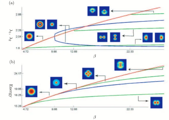
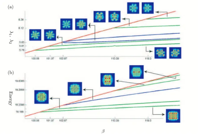
In Figure 4.1(a) and Figure 4.2(a) we plot the solution curves of eigenvalues for positive bound states versus the repulsive scattering length β∈ (4.2, 28) and (98, 125), respectively. Here the nodal domains of positive bound states are attached near the solution curves. Furthermore, in Figure 4.1(b) and Figure 4.2(b) the associated solution curves of energy versus β are plotted, respectively, and the level sets of two bound state solutions are attached near the solution curve of energy. In addition, the red and green lines in Figures 4.1 and 4.2, respectively, denote the primal stalks for the identical solutions and the bifurcation branch for the ground state solutions.
From the result of Theorem 3.4 we observe that the two-component BEC has positive bound state solutions u1 and u2with Πθ(u1) = u2 at β1∗(2) = 4.72, β2∗(2) =
12.88, β∗
3(2) = 22.33, β4∗(2) = 100.06, β5∗(2) = 101.97, β6∗(2) = 113.39 and β7∗(2) =
119.3, respectively.
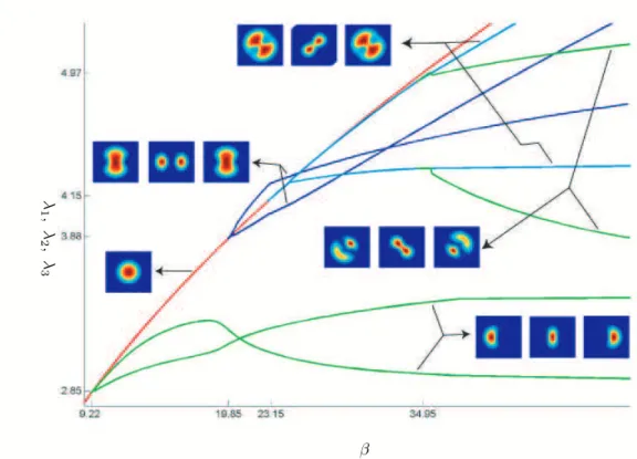
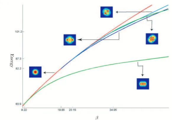
Example 4.2. For m = 3: Ω = [−5, 5] × [−4.8, 4.8], V1= V2 = V3 = x2+ y2,
α1 = α2 = α3 = 0.1, βkj = β, k 6= j, k, j = 1, 2, 3. The mesh size is the same
as in Example 4.1. As above, in Figures 4.3 and 4.4 we plot the solution curves of eigenvalues and energy versus β ∈ (8.7, 51), respectively. The nodal domains of positive bound states are attached near the solution curve of eigenvalues. The level sets of positive bound states are attached near the solution curve of energy. Similarly, the red and green lines in Figures 4.3 and 4.4, respectively, denote the primal stalks for the identical solutions and the bifurcation branch for the ground state solutions.
5. Conclusions. In this paper, we developed a continuation BSOR-Lanczos-Galerkin method for the computation of positive bound states of a multi-component BEC. The bifurcation diagram of positive eigenvectors/eigenvalues of NAEP and the associated energy functional of the time-independent CGPEs is traced by the pro-posed continuation method. Numerical experience shows that our method performs reliably and efficiently. Different from the NGF and TSSP methods for computing the ground states of a multi-component BEC only, the continuation method is pro-posed from the viewpoint of a nonlinear eigenvalue approach, which can be used for computing all possible positive bound states of a multi-component BEC. We proved that a phase separation of m ground/bound states will occur at a finite value of the
β β E ner gy λ 1, λ 2 (a) (b)
Fig. 4.1. m = 2. Solution curves of eigenvalues and energy versus β, for β ∈ (4.2, 28).
repulsive scattering length. For a two-component BEC, we also proved that two iden-tical ground/bound states will bifurcation into different Πθ-symmetry ground/bound
states.
In the future, we are interested in proving the existence of the Πθ-symmetry
phase separation for the ground/bound states of a multi-component BEC (m≥ 3).
REFERENCES
[1] A. Aftalion and Q. Du, Vortices in a rotating Bose-Einstein condensate: Critical angular velocities and energy diagrams in the Thomas-Fermi regime, Phys. Rev. A, 64 (2001), p. 063603.
[2] E. Allgother and K. Gerog, Numerical path following, Handbook of Nemerical Analysis, Edited by P. G. , 5 (1996).
[3] P. Ao and S. T. Chui, Binary Bose-Einstein condensate mixtures in weakly and strongly segregated phases, Phys. Rev. A, 58 (1998), pp. 4836–4840.
[4] W. Z. Bao, Ground states and dynamics of multi-component Bose-Einstein condensates, SIAM Multiscale Modeling and Simulation, (to appear).
[5] W. Z. Bao and Q. Du, Computing the ground state solution of Bose-Einstein condensates by a normalized gradient flow, SIAM J. Sci. Comput., (to appear).
[6] W. Z. Bao and D. Jaksch, An explicit unconditionally stable numerical methods for solving damped nonlinear Schrodinger equations with a focusing nonlinearity, SIAM J. Numer. Anal, 41 (2003), pp. 1406–1426.
[7] W. Z. Bao, D. Jaksch, and P. A. Markowich, Numerical solution of the Gross-Pitaevskii equation for Bose-Einstein condensation, J. Comput. Phys., 187 (2003), pp. 318–342. [8] W. Z. Bao and W. J. Tang, Ground state solution of trapped interacting Bose-Einstein
condensate by directly minimizing the energy functional, J. Comput. Phys., 187 (2003), 15
β E ner gy λ 1 , λ 2 (a) (b)
Fig. 4.2. m = 2. Solution curve of eigenvalues and energy versus β, for β ∈ (98, 125).
pp. 230–254.
[9] M. S. Bazaraa, H. D. Sherali, and C. M. Shetty, Nonlinear programming: theory and algorithms, Wiley, New York, 2 ed., 1993.
[10] A. Berman and R. J. Plemmons, Nonnegative matrices in the mathematical sciences, Aca-demic Press, New York, 1979.
[11] M. Berry, Large scale singular value computations, Internat. J. Supercomputer Appl., 6 (1992), pp. 13–49.
[12] T. F. Chan, Deflation techniques and block-elimination algorithm for solving bordered sungular systems, SIAM J. Sci. Stat. Compu., 5 (1984), pp. 121–134.
[13] S. M. Chang, C. S. Lin, T. C. Lin, and W. W. Lin, Segregated nodal domains of two-dimensional multispecies Bose-Einstein Condensates, (preprint).
[14] S. M. Chang, W. W. Lin, and S. F. Shieh, Fixed point methods for energy states of multi-component Bose-Einstein condensates, (preprint).
[15] M. L. Chiofalo, S. Succi, and M. P. Tosi, Ground state of trapped interacting Bose-Einstein condensates by an explicit imaginary-time algorithm, Phys. Rev. E, 62 (2000), pp. 7438– 7444.
[16] Y. S. Choi, J. Javanainen, I. Koltracht, M. Koˇstrun, P. J. Mckenna, and N. Savytska, A fast algorithm for the solution of the time-independent Gross-Pitaevskii equation, J. Comput. Phys., (to appear).
[17] B. D. Davidson, Large-scale continuation and numerical bifurcation for partial differential equations, SIAM J. Numer. Anal., 34 (1997), pp. 2008–2027.
[18] R. J. Dodd, Approximate solutions of the nonlinear Schr¨odinger equation for ground and excited states of Bose-Einstein condensates, J. Res. Natl. Inst. Stan., 101 (1996), pp. 545– 552.
[19] B. D. Esry and C. H. Greene, Spontaneous spatial symmetry breaking in two-component Bose-Einstein condensates, Phys. Rev. A, 59 (1999), pp. 1457–1460.
[20] B. D. Esry, C. H. Greene, J. P. Burke Jr, and J. L. Bohn, Hartree-Fock theory for double condensates, Phys. Rev. Lett., 78 (1997), pp. 3594–3597.
β λ 1, λ 2, λ 3
Fig. 4.3. m = 3. Solution curve of eigenvalues versus β, for β ∈ (8.7, 51).
[21] G. H. Golub and C. F. V. Loan, Matrix Computations, Johns Hopkins University Press, Baltimore, MD, 1989.
[22] S. Gutpa, Z. Hadzibabic, M. W. Zwierlein, C. A. Stan, K. Dieckmann, C. H. Schunck, E. G. M. van Kempen, B. J. Verhaar, and W. Ketterle, Radio-frequency spectroscopy of Ultracold Fermions, Science, 300 (2003), pp. 1723–1726.
[23] D. S. Hall, M. R. Matthews, J. R. Ensher, C. E. Wieman, and E. A. Cornell, Dynamics of component separation in a binary mixture of Bose-Einstein condensates, Phys. Rev. Lett., 81 (1998), pp. 1539–1542.
[24] H. B. Keller, Lectures on Numerical Methods in Bifurcation Problems, Springer-Verlag, Berlin, 1987.
[25] E. H. Lieb, R. Seiringer, and J. Yngvason, Bosons in a trap: a rigorous derivation of Gross-Pitaevskii energy functional, Phys. Rev. A, 61 (2000), p. 043602.
[26] C. J. Myatt, E. A. Burt, R. W. Ghrist, E. A. Cornell, and C. E. Wieman, Production of two overlapping Bose-Einstein condensates by sympathetic cooling, Phys. Rev. Lett., 78 (1997), pp. 586–589.
[27] B. N. Parlett, A new look at the Lanczos algorithm for solving symmetric systems of linear equations, Linear Algebra Appl., 29 (1980), pp. 323–346.
[28] Y. Saad, On the Lanczos method for solving symmetric linear systems with several right-hand-sides, Math. Comput., 48 (1987), pp. 651–662.
[29] B. I. Schneider and D. K. Feder, Numerical approach to the ground and excited states of a Bose-Einstein condensated gas confined in a completely anisotropic trap, Phys. Rev. A, 59 (1999), pp. 2233–2242.
[30] J. Stoer and R. Bulirsch, Introduction to Numerical Analysis, Springer-Verlag, Berlin, 2 ed., 1991.
[31] L. T. Watson, S. C. Billups, and A. P. Morgan, HOMEPACK: A suite of codes for globally convergent homotopy algorithms, ACM Trans. Math. Software, 13, pp. 281–310.
β
E
ner
gy