Hydrological Basis of Ecologically Sound Management of Soil and Groundwater
(Proceedings of the Vienna Symposium, August 1991). IAHS Publ. no. 202, 1991.
Sensitivity analysis of the surface water acidification model ILWAS in the saturated and unsaturated zone
F.J. CHANG
Department of Agricultural Engineering, Taiwan National University, Taipei, Taiwan, Republic of China
J.W. DELLEUR & A.R. RAO
School of Civil Engineering, Purdue University, West Lafayette, Indiana 47907, USA
ABSTRACT The ILWAS model was developed for the Electric Power Research Institute (EPRI) to predict the effect of acid deposition on surface water chemistry. This paper summarizes a sensitivity analysis conducted for the ILWAS model. The important variables in ILWAS were identified in an application of the model to the Panther Lake watershed in the Adirondack Mountains in the state of New York. The sensitivity analysis was found to be useful in eliminating the least sensitive hydrologie and chemical variables, thus simplifying the task of calibration of the model.
INTRODUCTION
To better understand the acidification process in a watershed, scientists have developed physically based mathematical models which quantify the linkage between atmospheric deposition and stream water quality (e.g. Chen et al-, 1983; Christophersen et al., 1982; Cosby et a l , 1985). The ILWAS (Integrated Lake-Watershed Acidification Study) model developed by Chen et al. (1983) is, at the present, the most comprehensive simulator. However, ILWAS requires extensive information on watershed physical and chemical characteristics which limits its use. Sensitivity analysis enables the identification of the important parameters in the model which require precise data. Less sensitive parameters can then be approximated by using the information in the literature or can be estimated by experience (Chang et al., 1986). Consequently, a sensitivity analysis was performed to simplify the ILWAS model by using data collected for the Panther Lake watershed in the Adirondack region of the state of New York.
THE ILWAS MODEL
The ILWAS (Integrated Lake-Watershed Acidification Study) was funded by the Electric Power Research Institute from 1977 to 1984. ILWAS was an interdisciplinary, multi-institutional study of three forested watersheds (Panther, Woods, Sagamore) in the Adirondack Mountains of New York State. Details of the model including its formulation were presented by Gherini et al. (1983) and by Goldstein et al. (1985). The following paragraphs give a brief overview of the model structure.
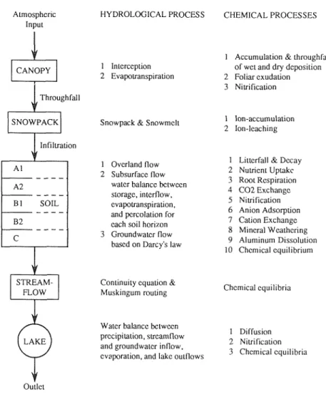
The ILWAS model conceptualizes a spatially heterogeneous watershed system in subcatchments, stream segments and lake(s). Each subcatchment contains compartments representing the canopy, the snowpack, and the soil
layers. The lake is divided into horizontally mixed layers to allow for calculation of temperature and water quality profiles. Basically, the model is composed of a hydrologie module and a chemical module, both split into a number of submodels. The hydrologie module routes precipitation from the vegetative canopy to lake outlet. It includes l) interception and évapotranspiration; 2) snowpack and snowmelt simulation; 3) overland flow; 4) subsurface water movement; 5) stream and lake routing.
The chemical module calculates the pH, the concentrations of alkalinity, the major cations (Ca2 +, M g2 +, K+, N a+, and N H j ) and anions (SOf-, N O J , Cl~,
and F~), nomomeric aluminum and its organic and inorganic complexes, organic acid analogues and dissolved inorganic carbon. It simulates 1) the canopy processes of accumulation and throughfall of wet and dry deposition, exudation, and wash-off; 2) the snowpack processes of ion-accumulation and ion-leaching; 3) the soil processes of cation exchange, anion adsorption, mineral weathering, C 02
exchange, and organic matter decomposition; 4) the chemical equilibria occurring in the aqueous phase. A schematic and processes summary of the IL WAS model are given in Fig. 1.
Atmospheric Input CANOPY V Throughfall SNOWPACK Infiltration ^f A l A2 Bl SOIL B2 STREAM-FLOW HYDROLOGICAL PROCESS 1 Interception 2 Evapotranspiration
Snowpack & Snowmelt
1 Overland flow 2 Subsurface flow
water balance between storage, interflow, évapotranspiration, and percolation for each soil horizon 3 Groundwater flow
based on Darcy's law
Continuity equation & Muskingum routing
Water balance between precipitation, streamflow and groundwater inflow, evaporation, and lake outflows
CHEMICAL PROCESSES
1 Accumulation & throughfall of wet and dry deposition 2 Foliar exudation 3 Nitrification
1 Ion-accumulation 2 Ion-leaching
1 Litterfall & Decay 2 Nutrient Uptake 3 Root Respiration 4 C02 Exchange 5 Nitrification 6 Anion Adsorption 7 Cation Exchange 8 Mineral Weathering 9 Aluminum Dissolution 10 Chemical equilibrium Chemical equilibria 1 Diffusion 2 Nitrification 3 Chemical equilibria Outlet
25 Sensitivity analysis of the surface water acidification model ILWAS
Because of its complexity, the ILWAS model requires extensive input data. For complete simulation, five input source files need to be read including control variables, lake-watershed characteristics, rate coefficients, meteorological data, and precipitation and air quality data.
SENSITIVITY ANALYSIS
The sensitivity of the ILWAS model to parameter variations was estimated as follows. First, the variable whose effect on the system response was to be estimated was selected and a reasonable range of values was defined for this variable. Next, the model was run for several values of this variable within the selected range. The simulated system responses were then examined. If the system responses showed a large variation, the selected input variable was defined as a sensitive variable. The sensitivity analysis was performed by using the Panther Lake watershed data (August 1978 to August 1981). The lake outlet hydrogen ion concentration was taken as the principal model output for evaluating the effects of changes in external input variables and internal watershed variables.
External input variables
The external input variables included six meteorological variables (precipitation, temperature, atmospheric pressure, cloud cover, dewpoint temperature and wind speed). The results show t h a t precipitation and temperature are the most sensitive input variables, and other meteorological variables are not sensitive. A result obtained from this analysis on monthly data is shown in Fig. 2 (a and b).
7.500-1 6.900- 6.300- 5.700- 5.100-a + A
111 111
\
I
! \ i i ORIGINAL AVE. RAIN AVE. TEMP3
K
a ORIGINAL 0 AVE. CLOUD A AVE. PRESSUR + AVE. WIN X AVE. 0EWP0IN * FINAL 80.00 MONTH (A) 20.00 MONTH (B)FIG. 2 Lake outflow pH as a function of time. Symbols indicate pH values obtained with monthly meteorological variables used by Chen et aL (1983) (ORIGINAL), with average annual value of indicated variable, and with the simultaneous use of four mean annual variables (FINAL).
It is evident (Fig. 2b) t h a t the average value (of observed values over 3 years) of one or all of the insensitive météorologie variables does not affect the pH value of the lake outflow very much. These 4 insensitive variables (atmospheric pressure, cloud cover, wind speed and dew point) only affect the lake evaporation rate. Consequently, if the watersheds do not have lakes, these 4 variables would not affect the result at all.
1 .DUU 1 .200 -Œ Ll_ UJ O ° 0.800-CD © A \ \ \
V\\
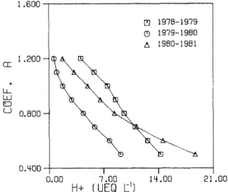
\ \ 1 1978-1979 1979-1980 1980-1981 1 0.00 7.00 , 14.00 H+ (UEQ L1) 21.00FIG. 3 Effect of changes of total soil depth on lake outflow H+
concentration. The existing soil depth is multiplied by the coefficient A shown in the ordinate.
2.400-C\J CJ 1.600- 0.000-0.00 7.00 H+ CONC, m 1978-1979 © 1979-1980 1980-1981 14.00 . UEQ L1) 21.00
FIG. 4 Effect of vertical hydraulic conductivity on basin outflow H+ concentration. The actual hydraulic conductivity if multiplied
27 Sensitivity analysis of the surface water acidification model ILWAS Internai watershed variables
Because of the great number of parameters (more than 130) in the several compartments comprising the model, it is impractical to conduct a sensitivity-analysis of all of them. However, some parameters in each compartment of the model are obviously key parameters because they influence or control others. For example, the plant type in the canopy, soil depth and the infiltration rate in the soil compartment, snowmelt rate in the snowpack compartment, and watershed slope in the surface flow are important parameters. With the most important parameters in each compartment selected, each of these parameters was changed individually and the ILWAS model simulation was performed. Finally, the results were compared to determine which compartment had the most effect on the lake outlet hydrogen ion concentration or pH value. The following results were obtained.
Soil compartment
The sensitivity analysis of the soil component was performed in 4 parts: a) the effect of the total depth, b) the effect of the thickness of each individual soil layer, c) the effect of reducing the number of soil layers and d) the effect of the hydraulic conductivity on lake outflow acidity. The depth of each layer appears explicitly in the water balance equation:
Aj Zj ^ = Aj P ^ - Aj Ep j - Pj Aj + 1 - Lj (l)
where
Aj = area of layer j (cm2 )
Zj = thickness of layer j (cm)
9\ = volumetric water content of layer j
P j - i = percolation from layer j - 1 into layer j Epj = évapotranspiration from layer j (cm s~l) Lj — lateral flow from layer j (cm3 s- )
The depth of each of the five layers was multipled by a coefficient varying from 0.40 to 1.20, all other parameters were kept constant, and likewise the hydraulic conductivity of all 5 soil layers was multipled by a coefficient varying from 0.1 to 2.0, all other parameters being kept constant. It is seen that the soil compartment has a large acid buffering capacity and demonstrates the most significant effect on the pH value of the basin outflow. In the Panther Lake watershed, as the total soil thickness increases, the acidity of lake outflow decreases (Fig. 3).
With increased vertical hydraulic conductivity, more water can percolate through deep soil, so the basin outflow becomes less acidic (Fig. 4).
Surface slope
The principal variable affecting the overland flow is the slope of the surface as the surface runoff is calculated from:
L o = i - W (D - D0)5/3 S1/2 n (2) where = surface runoff (cm3 s~ ' ) D Dn n S = depth of water (cm),
= max. detention storage (cm) = Manning's roughness coefficient = slope 8.0006 . 8.0006 8.0006 7 - 5.333- 4.000-• 0RIGINRH0.07) © MELT ROTE:0.01 + MELT RATE:0.10 0.00 12.00 24.00 MONTH 36.00
FIG. 5 Lake outflow pH for different snowmelt rate coefficients From these results, it is seen that a small a value (0.01) results in underestimation of the acidity peak and in a delay of its occurrence. The amplitude of the acidity peak is overestimated by a high a value (0.1).
The slope also appears in the expression for the lateral flow in the saturated soil layers:
Lj = Kj W SZsj (3)
where
Lj = the lateral flow from layer j
Kj = the saturated hydraulic conductivity of layer j (cm s"1)
W = the subcatchment width (cm) S = hydraulic gradient
29 Sensitivity analysis of the surface water acidification model ILWAS
The effect of changing the surface slope on the H+ concentration in basin
outflow is an increase in the acidity of the outflow as the slope decreases. As the value of the slope approaches 0.5 times the original slope, H+ concentration in
outflow eventually increased to 18 /xeq l- 1 from an original value 7.47 fxeq 1_ 1
for the first simulation year.
100.0-LL) CD Œ 50.0-X CJ LU O CC UJ Q_ 0.0- -50.0-H 1978-1979 © 1979-1980 A 1980-1981 0.00 7.00 < 14.00 H+ (UEQ L:1) 21.00
FIG. 6 Outflow H+ concentration as a function of percent change of
coniferous forest cover to deciduous forest cover.
Snowmelt
The snowmelt is estimated by the following relationships
M0 = a (T - Ts) [0.4 + sin (0.0087 /?)]
M
Mr = 0.0039 (T - Tg) PT (5) where M0 Mr a T TsP
P T— air temperature-induced melting rate in open areas (cm d a y- 1)
= rain-induced melting rate,o(cm d a y- 1)
= rate coefficient (cm d a y- 1 °C~})
= mean basin air temperature ( C)
= incipient snow formulation temperature ( C)
= aspect of the subcatchment (degrees measured clockwise from the North) = throughfall rate (cm d a y- 1) .
Panther Lake outflow exhibits sharp peaks of acidity during spring snowmelt. Several values of the snowmelt rate coefficient were investigated and the results are shown in Fig. 5.
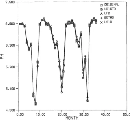
7.5006 . 9 0 0 - 6.300- 5.700- 5.100t,500 -H ORIGINAL O UD1STD A LFD + BETflD X LfllD 0.00 10.00 20.00 30.00 MONTH — 1 — 40.00 50.00
FIG. 7 Outflow pH using annual average values for four deciduous parameters. UDISTD is uptake of trees; LFD is litter fall rate; BETAD is foliar exudation rate; LAID is leaf area index.
Canopy
The forest cover on Panther Lake watershed includes 7 5 % hardwood (dominated by beech and maple), 14% mixed forest, 10% lowland coinferous forest and 1% wetland. The deciduous forest is thus the dominant species for this watershed. For deciduous canopy the acidity of the throughfall decreases with the leaf area index because of the important leaf exudation. In contrast, the coniferous canopy is particularly efficient in the collection of dry deposition, and because of higher leaf area index the coniferous canopy gives higher fluxes of all ionic species. To test the hypothesis that the canopy controls, in part the watershed outflow acidity, the proportion of coniferous cover was decreased to 3 % and increased up to 50%.
The canopy compartment demonstrated a smaller effect than other compartments. As the watershed vegetation type was changed from deciduous to coniferous, the basin outflow becomes acidic (Fig. 6); however, this change was not significant compared to the changes brought about by varying the soil depth or the watershed slope.
The sensitivity analysis was also performed to determine if an accurate determination of several monthly canopy parameters is necessary. The results obtained by using annual average values of the canopy parameters are not significantly different from those obtained using monthly values (Fig. 7).
31 Sensitivity analysis of the surface water acidification model ILWAS
CONCLUSIONS
The conclusions from the sensitivity analysis are:
(a) the amount of cloud cover, atmospheric pressure, wind speed, and dewpoint are not important meteorological inputs and can be replaced by yearly average values or by empirical equations;
(b) the soil buffering capacity demonstrates significant effect on the pH value of the basin outflow.
ACKNOWLEDGEMENTS The authors wish to express their appreciation to Dr. R.A. Goldstein of E P R I for the ILWAS code and Panther Lake watershed data, Dr. S.A. Gherini of Tetra Tech Inc. for his assistance. The Project was funded in part by the U.S. Geological Survey under Project G 1016-03 through the Purdue University Water Resources Research Center.
REFERENCES
Chang, F.J., Delleur, J.W. & Rao, A.R. (1986) Implementation, Sensitivity Analysis and Application of the "ILWAS" model of Acid Precipitation Impacts to Panther Lake and Walker Branch Watersheds. Purdue Univ. Water Resources Research Center Report No. 176.
Chen, C.W., Gherini, S.A. Hudson, J.M. & Dean, J.D.Q983) The Integrated Lake-Watershed Acidification Study. Vol. 1: Model Principles and Application Procedures. E P R I report EA-3221.
Christophersen, N., Seip, H.M. & Wright, R.F. 1982. A Model for Stream Water Chemistry at Birkenes, Norway, Wat. Resour. Res. 18, 977-996. Cosby, B.J., Wright, R.F., Hornberger, G.M. & Galloway, J.N. (1985)
Modeling the Effect of Acid Rain Deposition: Estimation of Long-Term Water Quality Responses in a Small Forest Catchment, Wat. Resour. Res.
21, 1591-1601.
Gherini, S.A., Mok, L., Hudson, R.J.M., & Davis, G.F. (1985) The ILWAS Model: Formulation and Application", Water. Air and Soil Pollutions 26, 425-459.
Goldstein, R.A., Gherini, S.A., Chen, C.W., Mok, L. & Hudson, J.M. (1984) Integrated Lake-Watershed Acidification Study (ILWAS): Mechanistic Ecosystem Analysis, Phil. Trans. R. Soc. London, B. Vol. 305, 409-425.