貼圖空間重要取樣之即時半透明顯像技術

全文

(1)國立交通大學多媒體工程研究所碩士論文. 貼圖空間重要取樣之即時半透明顯像技術 Real-Time Translucent Rendering using Texture Space Importance Sampling. 研究生：張志文指導教授：莊榮宏. 中華民國. 教授. 九十六. 年九月.

(2) 貼圖空間重要取樣之即時半透明顯像技術 Real-Time Translucent Rendering using Texture Space Importance Sampling. 研究生：張志文. Student： Chih-Wen Chang. 指導教授：莊榮宏. Advisor： Jung-Hong Chuang. 國立交通大學多媒體工程研究所碩士論文. A Thesis Submitted to Institute of Multimedia Engineering College of Computer Science National Chiao Tung University in partial Fulfillment of the Requirements for the Degree of Master in Computer Science. September 2007 Hsinchu, Taiwan, Republic of China. 中華民國九十六年九月.

(3) 貼圖空間重要取樣之即時半透明顯像技術. 研究生 : 張志文. 指導教授 : 莊榮宏博士林文杰博士. 國立交通大學資訊學院多媒體工程研究所. 摘要我們提出了一個利用貼圖空間的即時半透明材質顯像方法，貼圖空間的取得來自於模型表面參數化(surface parameterization)。我們將原先在三維模型表面上的積分轉換成一個在二維貼圖空間的積分式，並利用了以進入幅射量(irradiance)為基礎的重要取樣(importance sampling)來計算二維貼圖空間的積分。我們的架構可以在動態光源、動態材質以及即時的情況下利用少量的前置運算資料 (precomputation overhead)產生正確的半透明材質影像。當半透明現象明顯地由區域效果(local effects)所主導時，我們方法會受困於取樣數量需要相當大的問題。為了克服這問題，我們提出了混合式架構。在這架構裡，我們展示半透明材質顯像如何能被分解成區域效果(local effects)以及全域效果(global effects)。我們應用我們的貼圖空間重點取樣方法在全域效果的計算上。對於區域效果的計算則是結合兩個現有的即時半透明顯像方法[2,15]。我們的混合式架構在動態的材質下，可以用穩定效能與取樣數量來顯像半透明材質。. i.

(4) Real-Time Translucent Rendering using Texture Space Importance Sampling. Student: Chih-Wen Chang. Advisor: Dr. Jung-Hong Chuang. Institute of Multimedia Engineering College of Computer Science National Chiao Tung University. ABSTRACT We present a novel approach for real-time translucent rendering by using the texture space of the model surface, which is achieved from surface parameterization. We convert the integration over a 3D model surface into an integration over a 2D texture space. We apply importance sampling based on the irradiance for the integration over the texture space. We propose a threestage GPU-based rendering approach for translucent rendering. Our method can render accurate translucent image in real-time under dynamic environment about light and materials with lower precomputation overhead. Our method suffers from problem of sample number when the appearance of translucency is dominant to local effect. We propose hybrid method to overcome this problem. In our hybrid method, we show how the translucent rendering can be decomposed as local effects and global effects. We apply our GPU-based texture space importance sampling approach on the evaluation of global effects. The local effects are evaluated by the combination of two available methods for real-time translucent rendering [2, 15]. Our hybrid method can steadily render dynamic translucent material without changing the number of samples.. i.

(5) Acknowledgments. I would like to thank my advisors, Professor Jung-Hong Chuang, and Wen-Chieh Lin for their guidance, inspirations, and encouragement. I am grateful to Tan-Chi Ho for his comments and advices. Thanks to my colleagues in CGGM lab.: Yu-Shuo Lio, Chia-Lin Ko, Ya-Ching Chiu, Yung-Cheng Chen, Yueh-Tse Chen, Chih-Hsiang Chang, Hsin-Hsiao Lin, Kuang-Wei Fu, and Ying-Tsung Li for their assistances and discussions. I also want want to thank senior colleagues, Yong-Cheng Cheng, Yi-Chun Lin, Chao-Wei Juan, and Roger Hong. It is pleasure to be with all of you in the pass two years. Lastly, I would like to thank my parents for their love, and support.. ii.

(6) Contents 1. 2. Introduction. 1. 1.1. Thesis Overview . . . . . . . . . . . . . . . . . . . . . . . . . . . . . . . . .. 2. 1.1.1. Contribution . . . . . . . . . . . . . . . . . . . . . . . . . . . . . . .. 4. 1.1.2. Outline . . . . . . . . . . . . . . . . . . . . . . . . . . . . . . . . . .. 4. Background. 5. 2.1. Literature Review . . . . . . . . . . . . . . . . . . . . . . . . . . . . . . . . .. 5. 2.2. Fundamental of Realistic Image Synthesis . . . . . . . . . . . . . . . . . . . .. 7. 2.2.1. Radiometry . . . . . . . . . . . . . . . . . . . . . . . . . . . . . . . .. 7. 2.2.2. Reflectance Distribution Function . . . . . . . . . . . . . . . . . . . .. 10. 2.2.3. The Rendering Equation . . . . . . . . . . . . . . . . . . . . . . . . .. 12. 2.2.4. Tone-reproduction Operator . . . . . . . . . . . . . . . . . . . . . . .. 12. Light Transport of Subsurface Scattering . . . . . . . . . . . . . . . . . . . . .. 13. 2.3.1. The Volume Rendering Equation . . . . . . . . . . . . . . . . . . . . .. 15. 2.3.2. The Diffusion Approximation . . . . . . . . . . . . . . . . . . . . . .. 15. The Dipole Diffusion Approximation . . . . . . . . . . . . . . . . . . . . . . .. 17. 2.3. 2.4 3. Texture Space Importance Sampling Technique. 20. 3.1. Texture Space Importance Sampling . . . . . . . . . . . . . . . . . . . . . . .. 21. 3.1.1. 21. Reformulation of Rendering Equation . . . . . . . . . . . . . . . . . .. iii.

(7) 3.1.2 3.2. 3.3. 3.4 4. 5. Monte Carlo Importance Sampling . . . . . . . . . . . . . . . . . . . .. 23. Implemetation on GPU . . . . . . . . . . . . . . . . . . . . . . . . . . . . . .. 23. 3.2.1. Precomputation . . . . . . . . . . . . . . . . . . . . . . . . . . . . . .. 24. 3.2.2. Run-Time . . . . . . . . . . . . . . . . . . . . . . . . . . . . . . . . .. 25. Hybrid Approach . . . . . . . . . . . . . . . . . . . . . . . . . . . . . . . . .. 30. 3.3.1. Separation of Diffusion Function . . . . . . . . . . . . . . . . . . . . .. 30. 3.3.2. Method for Local Translucency . . . . . . . . . . . . . . . . . . . . .. 32. Discussion . . . . . . . . . . . . . . . . . . . . . . . . . . . . . . . . . . . . .. 35. Result. 41. 4.1. GPU-based Texture Space Importance Sampling . . . . . . . . . . . . . . . . .. 41. 4.2. Hybrid Method . . . . . . . . . . . . . . . . . . . . . . . . . . . . . . . . . .. 48. Conclusion. 50. 5.1. Summary . . . . . . . . . . . . . . . . . . . . . . . . . . . . . . . . . . . . .. 50. 5.2. Future Work . . . . . . . . . . . . . . . . . . . . . . . . . . . . . . . . . . . .. 51. Bibliography. 53. iv.

(8) List of Figures 1.1. Two different views of translucency without reflection. . . . . . . . . . . . . .. 2. 2.1. Plane angle and solid angle [18]. . . . . . . . . . . . . . . . . . . . . . . . . .. 9. 2.2. BRDF and BSSRDF [10]. . . . . . . . . . . . . . . . . . . . . . . . . . . . . .. 11. 2.3. An incoming ray is transformed into a dipole source for the diffusion approximation [19]. . . . . . . . . . . . . . . . . . . . . . . . . . . . . . . . . . . . .. 18. 2.4. The graph of Rd . . . . . . . . . . . . . . . . . . . . . . . . . . . . . . . . . .. 19. 3.1. An overview of our framework. Red points on the right image are generated samples. Model is Max Planck with marble material. The middle image of top row is visualization of normal direction. . . . . . . . . . . . . . . . . . . . . .. 24. 3.2. Inverse CDF sampling [3]. . . . . . . . . . . . . . . . . . . . . . . . . . . . .. 26. 3.3. Two different data orders for evaluating cumulative distribution function : Row major order and mipmap-based order. . . . . . . . . . . . . . . . . . . . . . .. 3.4. 27. Graph of weighting function and diffusion function. Rp is 2.4141 and K is 1.5 for weighting function. σa is 0.0024, σs0 is 0.70, and η is 1.3 for diffusion equation (parameters of red channel for skimmilk [10]). . . . . . . . . . . . . .. 31. 3.5. Graph of importance function for skimmilk material. . . . . . . . . . . . . . .. 32. 3.6. Image with (a) Full Rd function, (b) Local Rd function, and (c) Global Rd function. Model is 10mm MaxPlanck and material is Skimmilk. . . . . . . . .. v. 33.

(9) 3.7. Translucent Shadow Map [15] : (a) Irradiance map rendered from light view with filter. (b) A filter pattern with 21 samples. . . . . . . . . . . . . . . . . .. 34. 3.8. Overview of ”Efficient Rendering of Local Subsurface Scattering” [2]. . . . . .. 34. 3.9. Our method for local translucency. (a) Irradiance map rendered from light view with filter. (b) Filter pattern with 17(4x4+1) samples. . . . . . . . . . . . . . .. 35. 3.10 System overview of our hybrid method. The local and global effect are computed over the projection space and the texture space respectively. . . . . . . .. 38. 3.11 System overview of our ideal method. The local and global effect are both computed over the texture space. . . . . . . . . . . . . . . . . . . . . . . . . .. 39. 3.12 Diagram of adaptive sampling method on (a) texture space and (b) model space. Red point is current sample; Blue point is next sample; Green points are intersection of path and boundary of triangle. . . . . . . . . . . . . . . . . . . . . .. 40. 3.13 Result samples of adaptive sampling method on (a) texture space and (b) model space for one outgoing point at the forehead. The color in (b) is the visualization of diffusion function Rd(xi , xo ) for the outgoing point. . . . . . . . . . . . . . 4.1. 40. Result image using our method in Table 4.2. (a) MaxPlanck with skimmilk and 900 samples in 53.4 fps (b) Parasaur with skin1 and 1600 samples in 42.9 fps (c) TexHead with marble and 2500 samples in 19.4 fps.. 4.2. . . . . . . . . . . . .. 43. Top row are rendered by our method using 1600 samples in 29.8 fps. Second row are rendered by LTSM using 1600 samples in 8.0 fps. Third row are rendered by LSS[2] under same condition in 2.9 fps. . . . . . . . . . . . . . . . .. 4.3. Result image rendered by our method and by Jensen and Buhler [9] with 10mm igea. . . . . . . . . . . . . . . . . . . . . . . . . . . . . . . . . . . . . . . . .. 4.4. 45. Result image rendered by our method and by Jensen and Buhler [9] with 40mm igea. . . . . . . . . . . . . . . . . . . . . . . . . . . . . . . . . . . . . . . . .. 4.5. 44. 45. Result image using our method with different model size. Model sizes are 10, 25, 40, 55, 70mm from left to right. . . . . . . . . . . . . . . . . . . . . . . .. vi. 46.

(10) 4.6. Images of Parasaur model with skimmilk material is rendered with different texture resolution. . . . . . . . . . . . . . . . . . . . . . . . . . . . . . . . . .. 4.7. (a)(b) Images of cow head with marble material with difference parameterization result.(b)(d) Corresponding texture space of (a) and (b). . . . . . . . . . .. 4.8. 47. 47. Result images of skin1 material with different model scale. (a)(b)(c) are rendered by our texture space importance sampling method. (d)(e)(f) are rendered by our hybrid method. . . . . . . . . . . . . . . . . . . . . . . . . . . . . . . .. 4.9. 48. Result images of difference material with 10mm size. (a)(b)(c) are rendered by our texture space importance sampling method. (d)(e)(f) are rendered by our hybrid method. . . . . . . . . . . . . . . . . . . . . . . . . . . . . . . . . . .. vii. 49.

(11) List of Tables 2.1. Some examples of projected area. . . . . . . . . . . . . . . . . . . . . . . . .. 4.1. Performance of preprocessing in our method with difference model in millisecond (ms). . . . . . . . . . . . . . . . . . . . . . . . . . . . . . . . . . . . . .. 4.2. 8. 42. Performance of integration in our method with difference model in frame per second (fps). . . . . . . . . . . . . . . . . . . . . . . . . . . . . . . . . . . . .. 42. 4.3. Performance of preprocessing in LSS with difference model in millisecond (ms). 43. 4.4. Performance of integration in LSS with difference model in frame per second (fps). . . . . . . . . . . . . . . . . . . . . . . . . . . . . . . . . . . . . . . . .. viii. 43.

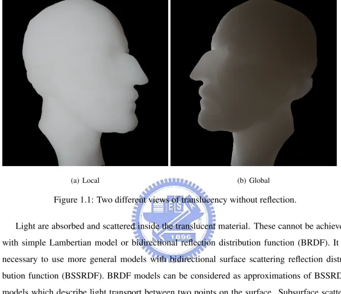
(12) CHAPTER. 1. Introduction Translucent materials are commonly seen in real world, e.g., snow, leaves, paper, wax, human skin, marble, and jade. When light transmits into a translucent object, it can be absorbed and scattered inside the object. This phenomenon is known as subsurface scattering. Subsurface scattering diffuses the scattered light and blurs the appearance of geometry details. Therefore, the appearance of translucent materials often looks smooth and soft, which is a distinct feature of translucent materials. Additionally, in some cases, light can pass through a translucent object and light the object from behind. These visual phenomena make rendering translucent objects a very complicate and important problem in computer graphics. It is necessary to simulate subsurface scattering to the appearance of translucent materials. Figure 1.1 shows two different views of a translucent object, demonstrating the local and global subsurface scattering effects. The appearance of translucency can be decomposed into two parts according to the cause of translucency. One is local effect that makes the geometry details blurred, which is mainly contributed from the nearby area of the outgoing point. The other is global effect that allows light to pass through translucent objects and light it from behind, which will lights up thin geometry details. In global effect, light rays are gathered from all the other points over the model surface.. 1.

(13) 1.1 Thesis Overview. (a) Local. 2. (b) Global. Figure 1.1: Two different views of translucency without reflection. Light are absorbed and scattered inside the translucent material. These cannot be achieved with simple Lambertian model or bidirectional reflection distribution function (BRDF). It is necessary to use more general models with bidirectional surface scattering reflection distribution function (BSSRDF). BRDF models can be considered as approximations of BSSRDF models which describe light transport between two points on the surface. Subsurface scattering can be treated as participating medium with specific boundary because of absorption and scattering. The shape of boundary also influences the appearance of translucency. Therefore, it needs huge amount of time to simulate the overall effect.. 1.1. Thesis Overview. Recent Researches on rendering translucent materials still suffer from the efficiency problem. Several papers [1, 7, 8, 14, 15, 21] tried to solve the problem using the pre-computation method, which requires 3D models and translucent materials to be static. Some other research [2, 15].

(14) 1.1 Thesis Overview. 3. evaluate subsurface scattering in run-time, but mostly focusing on local subsurface scattering rather than global subsurface scattering. To devise a real-time translucent rendering approach, we investigate that the major problem is sampling over the surface of an arbitrary 3D model. This inspires us to use the texture space of a model surface. Texturing is a technique for efficiently modeling the property of surface, which has been developed for real-time rendering and supported by graphics hardware for a long time. Surface parameterization was introduced to computer graphics as a method for mapping texture onto surface, which will generate a bijective texture space for given model surface. The texture space consists with the space of model surface. Integration over 2D texture space is easier, more efficient and without losing information of surface. In this thesis, we propose a real-time translucent rendering method using graphics hardware with low precomputation overhead. We convert the integration over a 3D model surface into an integration over a 2D texture space. Monte Carlo importance sampling is powerful and efficient method to accurately evaluate integration in most rendering application which generate realistic images, e.g., ray tracing, global illumination, direct illumination from environment maps. Hence, we apply Monte Carlo importance sampling based on irradiance for the integration over the 2D texture space, and propose a three-stage rendering approach for translucent rendering. We name this approach ”GPU-based Texture Space Importance Sampling”. Our texture space importance sampling method can render accurate global translucent effect with low sample number, but render local effect poorly with same number of samples. The necessary number of samples for accurate result will be very high if the appearance of translucency is dominated by the local effect. In order to overcome this drawback, we propose a hybrid method that evaluate the local effect and global effect with two difference approach. We show how the translucent can be decomposed as local effects and global effects. By this work, we apply our method on the rendering of global effects. For the local effects, we use the combination of the works of Mertens et al. [15] and the works of Dachsbacher and Stamminger [2]. We name this modified method ”Local Translucent Shadow Map”..

(15) 1.1 Thesis Overview. 1.1.1. 4. Contribution. The contributions of this thesis can be summarized as : • We reformulate the integration from a 3D model surface into a 2D texture space. • We apply Monte Carlo importance sampling to evaluate the integration over the 2D texture space based on the irradiance. • We implement our approach on graphics hardware and render accurate translucent image in real-time. • Our GPU-based texture space importance sampling method can render translucency with dynamic light and materials. • We show how the translucent can be decomposed as local effects and global effects. • We proposed a hybrid method to render local effects and global effects individually. • Our hybrid method can render accurate result image with stable sample number and performance. • We propose an efficient and accurate method for rendering translucent material with lower overhead than other precomputation-based approaches.. 1.1.2. Outline. The rest of the thesis is organized as follows : Chapter 2 gives the literature review, the background of realistic rendering and theory for translucent rendering. Chapter 3 presents the GPUbased texture space importance sampling method and hybrid method we propose for real-time translucent rendering, which includes algorithms and implementation details. Chapter 4 shows our experimental result from our approach. In the end, conclusions and future work are discussed in Chapter 5..

(16) CHAPTER. 2. Background. This chapter introduces the related work about translucent rendering. Then the background knowledge for realistic rendering and theory for translucent rendering will be introduced. It is divided into three parts: the first part is the foundation of physically accurate rendering in computer graphics. The second part describes essential theory for the rendering of translucent materials, the volume rendering equation. Finally, a practical equation, the dipole diffusion approximation, is introduced. The dipole diffusion approximation is proposed by Jensen et al.[10], on which recent relevant researches and ours are based to render translucent materials.. 2.1. Literature Review. Traditionally, subsurface scattering has been approximated as Lambertian diffuse reflection or BRDF models. Lambertian or BRDF models consider only the reflectional relation between incident and outgoing radiance at single point. Nicodemus et al. [17] proposed BSSRDF model which considers the light scattering relation between the incident flux at a point and the outgoing radiance at another point on surface. They formulated the subsurface scattering equation. 5.

(17) 2.1 Literature Review. 6. without analytic solution. Hanrahan and Krueger [6] first proposed a method for simulating subsurface scattering by tracing light rays inside an object. Their approach, however, can only be applied to thin objects, such as leaf and paper. Light scattering in thick objects is too complicated to be fully traced. Recently, Jensen et al. [10] proposed an analytic and complete BSSRDF model, in which BSSRDF is divided into a single scattering term and a multiple scattering term. Single scattering term is contributed by light that scatters only once inside an object; Light rays that scatter more than once contribute to the multiple scattering term. Jensen et al. approximated the multiple scattering term as a dipole diffusion process. The diffusion approximation works well in practice for highly scattering media where ray tracing is computationally expensive [6, 20]. This approach is much faster than Monte Carlo ray tracing, because the scattering effect is evaluated without simulating the scattering situation inside the model. Several recent papers exploit the diffusion approximation to render translucent materials [1, 2, 7–9, 13–16, 21]. Jensen and Buhler [9] proposed a two-stage hierarchical rendering technique to efficiently render translucent materials in interactive frame rate with acceptable error bound. Keng et al. [12, 13] further improved this approach using a cache scheme. Lensch et al. [14] modified Jensen’s formulation into a vertex-to-vertex throughput formulation. They precompute the throughput and use the information to render in real-time frame rate. Carr et al. [1] further improve this approach by using parallel computation and graphics hardware. Hao et al. [7, 8] precompute the contribution of light from every possible incoming directions and use spherical harmonics to compress the data. With the precomputation, images can be rendered in real-time. Wang et al. [21] presented a technique for interactive rendering of translucent objects under all-frequency environment maps. They reformulate both the equation of single and multiple scattering terms based on the precomputed light transport. Most of the papers above use precomputation techniques and require the scene and property of model to be static. Both Mertens et al. [15] and Dachsbacher and Stamminger [2] proposed methods for computing translucent effects in run-time without precomputation. Their ideas are similar but using different approaches. Mertens et al. [15] focused on local subsurface.

(18) 2.2 Fundamental of Realistic Image Synthesis. 7. scattering. They render the irradiance image from light view and evaluate the local subsurface scattering by sampling the irradiance in a small area around the outgoing point. Dachsbacher and Stamminger [2] extended the concept of shadow map by first rendering the irradiance image from light view and then evaluating translucent effects by applying filtering around the projected position of the outgoing point on irradiance image. This approach can catch both local and global subsurface scattering, but the effects of global subsurface scattering are not preserved sufficiently because only an area of single incident point, rather than all incident points, is taken into account.. 2.2. Fundamental of Realistic Image Synthesis. In this section, we first introduce radiometry and basic terminologies used to describe light. We then briefly discuss the interaction between light and surface, and introduce the rendering equation. Finally, we talk about how to display the high-dynamic-range images with energy information on low-dynamic-range devices, which is also known as tone-reproduction operator. [3, 18]. 2.2.1. Radiometry. Since the middle of the sixteenth century, there have been several attempts to develop models for the behavior of light, such as geometry optics, wave optics, electromagnetic optics, and photon optics [10]. The basic terminology used among them is radiometry, a measurement of optical radiation, which is electromagnetic radiation within the frequency range between 3 × 1011 and 3 × 1016 Hz. This range corresponds to wavelength between 0.01 and 1000 micrometers (µm), and includes the regions commonly called the ultraviolet, the visible, and the infrared.. Before we introduce the quantities and units used in radiometry, we explain two basic terms: projected area and solid angle..

(19) 2.2 Fundamental of Realistic Image Synthesis. 8. Projected area is defined as the orthogonal projection of a surface onto a plane perperidicular to the unit direction. The differential form is dAproj = cos(β)dA, where β is the angle between the local surface normal and the line of sight. We can integrate dAproj over the visible surface area to get Aproj =. Z. cos(β)dA. A. Here we list some examples of projected area assuming that there are no obstacles in the line of sight (Table 2.1). Shape. Area (visible parts). projected area. Flat rectangle A = Length · W idth Aproj = Length · W idth · cosβ Circular disc. A = πr2. Aproj = πr2 cosβ. Sphere. A = A = 2πr2. Aproj = 2πr2 cosβ. Table 2.1: Some examples of projected area. Solid Angle is an extension of the plane angle from two dimensions to three dimensions. Recall the definition of a plane angle [18] is ”One radian is the plane angle between two radii of a circle that cuts off on the circumference an arc equal in length to the radius.” The definition of a solid angle [18] extends to ”One steradian (sr) is the solid angle that, having its vertex in the center of a sphere, cuts off an area on the surface of the sphere equal to that of a square with sides of length equal to the radius of the sphere.” The solid angle of an object is thus the area of the projection of the object onto a unit sphere. Note that two objects different in shape can still subtend the same solid angle. We can think of the differential solid angle as representing both a direction and an infinitesimal area on the unit sphere, as seen in Figure 2.1. The most basic quantity in radiometry is the photon. The energy eλ of a photon with a wavelength λ is eλ = hc/λ where h is Planck’s constant, and c is the speed of light. eλ is measured in joules (J). Spectral radiant energy Qλ in nλ photons with wavelength λ is Qλ = nλ eλ = nλ. hc . λ.

(20) 2.2 Fundamental of Realistic Image Synthesis. 9. Figure 2.1: Plane angle and solid angle [18]. Radiant energy Q is the energy computed by integrating the spectral radiant energy over all possible wavelengths: Q=. Z ∞ 0. Qλ dλ.. Radiant flux or radiant power Φ is the time rate of flow of radiant energy: Φ=. dQ , dt. where t is measured in second. Radiant flux is often just called the flux.. Radiant flux area density M , B or E is defined as the differential flux per differential area at a surface location x: M (x) = B(x) = E(x) =. dφ , dA. where M and B is referred to as radiant existence or radiosity, which is the flux leaving from a surface, E is referred to as irradiance, which is the flux arriving at a surface.. Radiant intensity I is defined as the differential flux per differential solid angle dω : I(ω) =. dφ . dω.

(21) 2.2 Fundamental of Realistic Image Synthesis. 10. Radiance L is defined as the differential flux per differential projected area per differential solid angle: L(x, ω) =. d2 φ . cosθdAdω. Radiance is a five-dimensional quantity (three for position and two for direction), which is the most important quantity in radiometry, since it could most closely represent the color of an object. Most light receivers, such as cameras and the human eye, are sensitive to radiance, while the response curve of these sensors may be different.. 2.2.2. Reflectance Distribution Function. The interaction between light and material is complicated in the real world. In this section, we will introduce two theoretical models used to describe the scattering and reflection of light by materials.. The Bidirectional Scattering Reflectance Distribution Function (BSSRDF) is the most general model of light transport, which relates the differential reflected outgoing radiance dLr at xo in direction ωo to the differential incident flux dΦi at xi from direction ωi [17]: S(xi , ωi , xo , ωo ) =. dL(xo , ωo ) . dΦ(xi , ωi ). The BSSRDF is eight-dimensional (four for two positions in local two-dimensional coordinates and four for two directions) and costly to evaluate, so there are only few papers in computer graphics that address explicit computation of BSSRDF. The Bidirectional Reflectance Distribution Function (BRDF) is an approximation of the BSSRDF, which assumes that light enters and leaves the material at the same point (i.e., xo = xi ). BRDF reduces the BSSRDF to a six-dimensional function (two for position in local two-dimensional coordinates, four for two directions) [17]: fr (x, ωi , ωo ) =. dL(x, ωo ) dL(x, ωo ) = . dEi (x, ωi ) Li (x, ωi )(ωi ·N )dωi.

(22) 2.2 Fundamental of Realistic Image Synthesis. 11. Figure 2.2: BRDF and BSSRDF [10]. where N is the normal at x. BRDF defines the relationship between differential outgoing reflected radiance and differential incident irradiance and is widely used in photo-realistic rendering. It has some interesting properties: • The BRDF can take any positive value, and varies with wavelength. • The BRDF is independent of the direction, in which light flows, fr (x, ωi , ωo ) = fr (x, ωo , ωi ). This is a fundamental property that is used by most global illumination algorithms, since that makes it possible to trace light path in both directions. • The value of the BRDF for some incident direction ωa is independent of the possible presence of irradiance along other incident direction ωb , so the BRDF behaves as a linear function with respect to all incident directions. We can compute the reflected radiance Lr in any direction by integrating the incident radiance Li : Lr (x, ωo ) =. Z Ω. fr (x, ωi , ωo )Li (x, ωi )(ωi ·N )dωi .. • The BRDF must satisfy the constraint of energy conservation : Z Ω. fr (x, ωi , ωo )(ωo ·N )dωo ≤1, ∀ωi .. (2.1).

(23) 2.2 Fundamental of Realistic Image Synthesis. 2.2.3. 12. The Rendering Equation. The rendering equation is a mathematical formulation of the steady-state equilibrium distribution of energy in a scene without participating media. It forms the mathematical basis for producing realistic images. The rendering equation expresses the outgoing radiance Lo as the sum of the emitted radiance Le and the reflected radiance Lr : Lo (xo , ωo ) = Le (xo , ωo ) + Lr (xo , ωo ). By using BRDF model and Equation 2.1 to replace the reflected radiance we get : Z. Lo (xo , ωo ) = Le (xo , ωo ) +. Ω. fr (xo , ωi , ωo )Li (xo , ωi )(ωi ·N )dωi .. (2.2). This is the basic form of the rendering equation describing all light transport in a scene without participating media. The major difference between BRDF and BSSRDF is how to formulate the reflected radiance. In the case of BSSRDF, we can get : Lo (xo , ωo ) = Le (xo , ωo ) +. 2.2.4. Z Z A. Ω. S(xo , ωi , xi , ωo )Li (xi , ωi )(ωi ·N )dωi dxi .. (2.3). Tone-reproduction Operator. Up to now, all we discuss about is computing the correct radiometric values for each pixel in the final images. These values are measured in radiance that can be computed at a specific point in space and in a specific direction. However, these physically based radiance values do not appropriately indicate how the human eye perceives the environment because the human visual system is very complicated and does not simply respond linearly to changing levels of illumination. Tone-reproduction operator, or tone-mapping operator, is therefore presented to solve this problem by exploiting the limitations of the human visual system to display a high-dynamicrange picture onto a low-dynamic-range display device. There are various tone-mapping operators have been presented in literatures. In general, they function by creating a local scale.

(24) 2.3 Light Transport of Subsurface Scattering. 13. factor for each pixel in the high-dynamic range image based on the local adaptation luminance of the pixel and the high-dynamic-range value of the pixel. The resulting value produced by tone-mapping operators is typically an RGB value in the range from 0 to 1 that can be displayed on the output device.. 2.3. Light Transport of Subsurface Scattering. With rendering equation we can computed accurate radiance for each pixel and generate color image by applying tone-reproduction operator. Before simulating translucency, we must have accurate BSSRDF model. In this section, we deals with the light transport theory for translucent materials, and the construction of BSSRDF model. In light transport theory, photons traveling in a medium will collide with the medium, causing them to be absorbed or change directions (scattering). Absorption means the energy carried by photons is converted into other types of energy, for instance, the energy could be converted from radiation to kinetic energy of particles in the medium. The probability that a photon gets absorbed in a medium, per unit of distance along its direction of propagation, is called the absorption coefficient σa (x) and the probability that a photon gets scattered in a medium is called the scattering coefficient σs (x). These two coefficients are all measured in the unit of length, e.g., 1/m or 1/mm. This means that a photon traveling a distance ∆x in a medium has a chance σa ∆x and σs ∆x of being absorbed and scattered, respectively. The change in radiance L in the direction w due to out-scattering could be modeled as the following equation: (ω·∇)L(x, ω) = −σs (x)L(x, ω), and the change due to absorption could be modeled as: (ω·∇)L(x, ω) = −σa (x)L(x, ω)..

(25) 2.3 Light Transport of Subsurface Scattering. 14. We often combine the two coefficients to the extinction coefficient σt (x) as σt (x) = σs (x) + σa (x), and the combined loss in radiance is given by: (ω·∇)L(x, ω) = −σt (x)L(x, ω).. (2.4). On the other hand, when photons move through the media, there will also be a gain in radiance due to in-scattering of light from other directions. The change due to in-scattering is modeled by: (ω·∇)L(x, ω) = σa (x). Z Ω. p(x, ωi , ω)Li (x, ωi )dωi ,. (2.5). where the incident radiance, Li , is integrated over all possible directions. p(x, ω, ωi ) is the phase function describing the distribution of the scattered light. We assume that the phase function is normalized,. R Ω. p(x, ωi , ω)dωi = 1, and is a function only of the phase angle, p(x, ωi , ω) =. p(x, ωi ·ω). The mean cosine g of the scattering angle is defined as g =. R Ω. (ωi ·ω)p(ωi ·ω)dωi .. It indicates the type of scattering in the medium. If g is positive, the medium is predominantly forward scattering; if g is negative, the medium is predominantly backward scattering; if g equals zero, the phase function is constant and the medium results in isotropic scattering. Most translucent materials are strongly forward scattering with g ¿ 0.7. Such strongly peaked phase functions are costly to simulate in media with multiple scattering since the probability of sampling in the direction of the light source will be low in most situations. In this case we can benefit from a powerful technique known as the similarity of moments, which allows us to change the scattering properties of the medium without significantly influencing the actual distribution of light [9, 10]. Specifically, we can modify the medium to have isotropic scattering by changing the scattering coefficient to σs0 = σs (1 − g), where σs0 is the it reduced scattering coefficient. The absorption coefficient remains unchanged, and we get the reduced extinction coefficient σt0 = σs0 + σa ..

(26) 2.3 Light Transport of Subsurface Scattering. 15. In addition to the gain in radiance due to in-scattering, there is also a gain in radiance due to volume emission Le from the medium (i.e., a flame), and it is given by: (ω·∇)L(x, ω) = σa (x)L(x, ω).. (2.6). By combining Equation 2.4,2.5, and 2.6 we get a linear integro-differential equation, which is the so called light transport equation, or radiative transport equation: (ω·∇)L(x, ω) = σa (x)L(x, ω) − σt (x)L(x, ω) + σa (x). 2.3.1. Z Ω. p(x, ωi , ω)Li (x, ωi )dωi .. (2.7). The Volume Rendering Equation. In computer graphics, the light transport equation is often represented in another form, which is derived by integrating Equation 2.7 on both sides for a segment of length s subject to the appropriate boundary conditions [3, 10]. L(x, ω) =. R s −τ (x,x0 ) e σ. 0. )Le (x0 )dx0. +. R s −τ (x,x0 ) e σ. 0. ). 0. 0. a (x. a (x. R Ω. p(x0 , ωi , ω)L(x0 , ωi )dωi dx0. (2.8). + e−τ (x,x+sω) L(x + sω, ω) where τ (x, x0 ) (often called optical depth) is given by: τ (x, x0 ) =. R x0 x. σt (z)dz. Equation 2.8 is. the so called volume rendering equation, which is much more complicated than the rendering equation because the light is influenced by light at every point in space, not just the points on other surface.. 2.3.2. The Diffusion Approximation. The light transport equation, either in the form of Equation 2.7 or Equation 2.8, is a fivedimensional equation with integrals, which is very difficult to solve even when the light is scattered isotropically in the medium. It also difficult to construct analytic BSSRDF model from Equation 2.8. Therefore, we need to use the diffusion approximation to make it feasible.

(27) 2.3 Light Transport of Subsurface Scattering. 16. to solve the light transport equation [10, 20]. The diffusion approximation is based on the observation that as the number of scattering events increases, the angular dependence tends to be smoothed out, i.e., the light distribution in highly scattering media tends to become isotropic. The diffusion approximation begins by dividing the radiance into two components: the unscattered radiance (or reduced radiance) Lu and the scattered radiance (or diffuse radiance) Ld . The un-scattered radiance is the radiance that reaches point x directly from a light source, or from the boundary of the participating medium. It decreases exponentially with the distance traveled through the medium : 0. Lu (x + ∆x, ω) = e−σt ∆x Lu (x, ω). The diffuse radiance is radiance scattered one or more times in the medium. As stated above, after many scattering events, the angular dependence of diffuse radiance tends to be smoothed out, so the diffusion approximation can use the first four terms of the spherical harmonic expansion to represent Ld : Ld (x, ω)≈. 3→ 1 − φ(x) + E (x) · ω. 4π 4π. (2.9). where phi(x) = Ω Ld (x, ω 0 )dω 0 is the 0th-order spherical harmonic, called the radiant R → − fluence and E (x) = Ω Ld (x, ω 0 ) · ω 0 dω 0 is the 1st-order spherical harmonic, called the vector R. irradiance. Substituting the diffusion approximation (Equation 2.9) to the light transport equation (Equation 2.7) yields the classic diffusion equation: D∇2 φ(x) = σa φ(x) − S0 (x) + 3D∇S1 (x),. (2.10). where D = 1/3σt0 ; and S0 (x) and S1 (x) represents the 0th -order and the 1st -order spherical harmonic expansions of the source term, respectively. The diffusion equation can be solved analytically for special cases [10], or numerically by using a multi-grid method [20]. However, in the case of translucent materials, we are only.

(28) 2.4 The Dipole Diffusion Approximation. 17. interested in the outgoing radiance at the material surface as a function of the incoming radiance. Therefore we can further simplify the solution of the diffusion equation using the dipole diffusion approximation, which we will describe in next section.. 2.4. The Dipole Diffusion Approximation. The dipole diffusion approximation, which approximates the volumetric source distribution using a dipole (i.e. two point sources), was originally developed in medical physics community. The idea was proposed by Eason et al. [4] for modeling the back-scattering of light by blood. Farrell et al. [5] used a single dipole to represent the incident source distribution for the noninvasive determination of tissue optical properties in vivo. Jensen et al. [10] then introduced the dipole diffusion approximation to computer graphics community for modeling the subsurface light transport. The dipole diffusion approximation consists of positioning two point sources near the surface to approximate an incoming light see Figure 2.3. One point source, the positive real light source, is locate at the distance zr beneath the surface, and the other one, the negative virtual light source, is located above the surface at a distance zv . By using the dipole diffusion approximation to solve diffusion equation, we can get the following expression for the radiant exitance Mxi (xo ) at surface location xo due to incident flux Φ(xi ) at xi (see [9, 10] for the details of derivation): dMxi (xo ) = where α0 =. e−σtr sv e−σtr sr α0 [zr (1 + σtr sr ) 3 + zv (1 + σtr sv ) 3 ]dΦ(xi ). 4π sr sv. (2.11). σs0 σt0. is the reduced albedo which describe the relative importance of scattering versus q √ absorption; σtr = 3σa σt0 is the effective transport coefficient; sr = r2 + Zr2 and sv = q. r2 + Zv2 are the distance from xo to the positive real light source and the negative virtual light. source; r = kxo + xi k is the distance from xo to xi ; zr = lu and zv = (1 + 4A/3)lu are the distance from the dipole source to the surface as shown in Figure 2.3. The mean-free path lu = 1/σt0 is the average distance at which the light is scattered. Finally, the boundary condition.

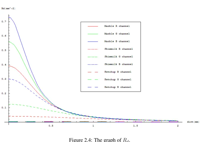
(29) 2.4 The Dipole Diffusion Approximation. 18. Figure 2.3: An incoming ray is transformed into a dipole source for the diffusion approximation [19]. for mismatched interfaces is taken into account by the A term which is computed as A =. 1+Fdr , 1−Fdr. where the diffuse Fresnel term Fdr is approximated from the relative index of refraction η by : Fdr = −. 1.440 0.710 + 0.668 + 0.0636η. + η2 η. By using Equation 2.11, the subsurface illuminance then could be computed as: S(xo ) =. R. =. R. =. R. =. R. A. dM( xi )(xo ). α0 A 4π [zr (1. + σtr sr ) e. −σtr sr. s3r. α0. 0 A E (xi ) 4π [zr (1 + σtr sr ) A. + zv (1 + σtr sv ) e e−σtr sr s3r. −σtr sv. s3v. ]dΦ(xi ) −σtr sv. + zv (1 + σtr sv ) e. s3v. (2.12). ]dxi. E 0 (xi )Rd (xi , xo )dxi. where E 0 (xi ) is the inside irradiance at point xi . Rd (xi , xo ) is the diffuse BSSRDF defined as the ratio of radiant exitance to incident flux. Figure 2.4 shows the graph of Rd which has exponentially decreasing property..

(30) 2.4 The Dipole Diffusion Approximation. 19. Substituting Fresnel transmittance into 2.9. Finally, the diffuse radiance L(xo , ωo ) can be computed as: L(xo , ωo ) = Ft (η, ωo )B(xo ) B(xo ) E(xi ). =. R. =. R. A Ω. E(xi )Rd (xi , xo )dxi. (2.13). Ft (η, ωi )(ωi ·Nxi )L(xi , ωi )dωi. where E(xi ) is the irradiance at incident point xi ; and B(xo ) is the radiosity at outgoing point xo . The dipole diffusion approximation introduced by Jensen et al. [10] is widely used by following researchers in computer graphics community. Our framework is based on Equation 2.13.. Figure 2.4: The graph of Rd ..

(31) CHAPTER. 3. Texture Space Importance Sampling Technique. Our development of a texture space importance sampling technique for real-time translucent rendering is based on the following observations : • According to the works of Jensen et al.[9, 10], the evaluation of translucency is an integration over a model surface. Sampling and integration over the model surface is complicated and time consuming. • A three-dimensional model surface can be converted into two-dimensional texture space by parameterization. Integration over the texture space is easier, more efficient and without loss of information of the 3D surface. • Monte Carlo importance sampling is a powerful and efficient method to accurately evaluate integration in most rendering applications. With appropriate probability density function and sampling strategy, Monte Carlo importance sampling can reduce the required number of samples and speed up computation.. 20.

(32) 3.1 Texture Space Importance Sampling. 21. • Graphics hardware is a powerful tool for parallel computation, and is widespread used in real-time rendering and general purpose computation. For the sake of efficiency, we render translucent effects by evaluating the integration over 2D texture space. We can achieve real-time performance by using the parallel computation of Monte Carlo importance sampling and graphics hardware. In this chapter, we propose a GPU-based texture space importance sampling method for rendering translucent materials. When the appearance of translucency is dominated by the local effect, the necessary number of samples for accurate result will be very high. To overcome this efficient issue, we also propose a hybrid approach to reduce the necessary number of samples.. 3.1. Texture Space Importance Sampling. In this section, we describe our texture space importance sampling method for translucent rendering. First we convert the integration over the model surface in Equation 2.13 into the integration over texture space. Monte Carlo importance sampling is applied based on the irradiance function to evaluate the integration over the texture space. Finally, we adopt the mipmap technique and GPU acceleration to develop a three-stage translucent rendering approach.. 3.1.1. Reformulation of Rendering Equation. Integration of outgoing radiosity B(xo ) in Equation 2.13 is the most important process to render translucent materials. However, it is also computationally expensive to sum up the contributions from all surface points. A straightforward way to compute the radiosity is to simply evaluate integration [3, 11] using uniform sampling over the object surface, as proposed by Jensen and Buhler [9]. A spatial hierarchy on the samples can be built to speed up the computational performance. However, this approach has several drawbacks. First, uniform sampling over a 3D surface is time consuming. Geometry modeling techniques need to be applied to ensure that mutual distance among sam-.

(33) 3.1 Texture Space Importance Sampling. 22. ples is the same. Second, the number of samples over the model surface could be very high if an accurate integration result is needed, especially when the appearance is dominated by the local translucent effect. It would require lots of time and memory to maintain the data structure of samples. We avoid the expensive sampling process over a model surface by convert the integration into the texture space. Since the input model is triangle mesh, the integration can be represented as summation of triangle faces. B(xo ) =. NF Z X j=1 Fj. E(xi )Rd (xi , xo )dxi ,. (3.1). where NF is the total number of triangle faces, and Fj is the area of the jth triangle face. After parameterization, each triangle face will be associated unique texture coordinate, which is bijective to the 3D model space. In theory, we can directly convert the integration of triangle face into texture space, but triangle area in texture space may be shrunk or enlarged in the parameterization process. In order to obtain correct integration results, we scale the area size for each triangle face. B(xo ) =. AjS Z E(xi )Rd (xi , xo )dxi , j j=1 AT Tj NF X. (3.2). where AjS and AjT are area size of triangle face on 3D model surface and on 2D texture space respectively; Tj is the jth triangle face in texture space. The texture space usually contains some regions that are not mapped to any triangle face. In these regions, the area size of triangle face AjS and irradiance E(xi ) are both zero. These area do not influence the integration of the whole texture space because of the zero value. Therefore, we can merge integration of each triangle face into a unique texture space. B(xo ) = =. PNF AjS R j=1 Aj T. R T. Tj. E(xi )Rd (xi , xo )dxi. (3.3). E 0 (xi )Rd (xi , xo )dxi. where T is the texture space of the model surface; E 0 (xi ) = AjS E(xi )/AjT is the product of the irradiance term and the area scaling term..

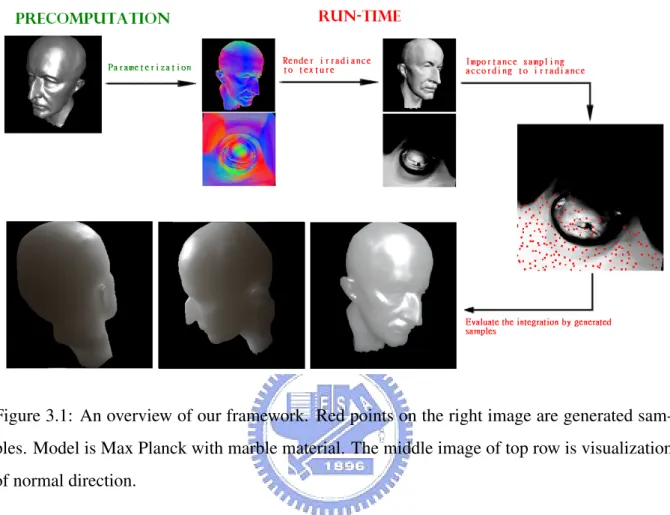
(34) 3.2 Implemetation on GPU. 3.1.2. 23. Monte Carlo Importance Sampling. We apply importance sampling [3, 11] to Equation 3.3 to reduce the number of samples without losing too much accuracy. Importance sampling distributes samples according to a probability density function over the space of integration. When the number of samples increases to infinite, the result of importance sampling will converge to the true integral value. We need to define an appropriate probability density function to capture the appearance of translucency. Importance sampling can not be applied to the product of irradiance function E 0 (xi ), and diffusion function Rd(xi , xo ). Comparing these two functions, we observe that importance sampling based on Rd(xi , xo ) will force samples to locate near the outgoing point, as shown in the work of [2, 15]. The feature is more biased to local subsurface scattering. On the other hand, importance sampling based on the irradiance function is more biased to the effect of global subsurface scattering. Therefore, we define our probability density function over texture to be proportional to the value of the irradiance function E 0 (xi ). Note that samples generated according to irradiance can be shared for every outgoing point since the irradiance function remains unchanged in run-time. 0. p(xi ) = E (xi )/. Z T. E 0 (xi )dxi. (3.4). With N samples distributed based on the probability density function, the integration of outgoing radiosity can be derived as follow : B(xo ) = = 0 where Eavg =. 3.2. R T. 1 PN E 0 (xi )Rd (xi ,xo ) i=1 N p(xi ) 0 PN Eavg i=1 Rd (xi , xo ) N. (3.5). E 0 (xi )dxi is the integration of irradiance over texture space.. Implemetation on GPU. In this section, we will describe implementation details of our approach. Figure 3.1 shows the overview of our approach that consists of a precomputation step and three-stage translucent.

(35) 3.2 Implemetation on GPU. 24. Figure 3.1: An overview of our framework. Red points on the right image are generated samples. Model is Max Planck with marble material. The middle image of top row is visualization of normal direction. rendering in run time. In the precomputation, we need generate a texture space for an input mesh. The color images of the second column of top row in Figure 3.1 are visualization of normal direction in 3D space and texture space. In run-time, we develop a three-stage translucent rendering method on GPU, including rendering the irradiance to texture space, importance sampling according to the irradiance, and evaluating of the integration.. 3.2.1. Precomputation. In our design of texture space, we can use any kind of parameterization method, as long as every triangle face is mapped on texture space and no overlapping for any two triangle faces. We can use maya auto-mapping method, handmade texture mapping or method proposed by research of parameterization etc... The triangle mesh and associated texture coordinates will be the input.

(36) 3.2 Implemetation on GPU. 25. of the run-time rendering. The quality of parameterization affects the accuracy of our importance-sampling-based integration. If triangles are shrunk or enlarged too much, undersampling or supersampling may happen inside those triangles. Therefore, area preserving parameterization or signal specified parameterization are preferred more accurate integration. In our implementation, an area preserving parameterization method proposed by Yoshizawa et al. [22] is used.. 3.2.2. Run-Time. In run-time, we develop a three-stage translucent rendering method on GPU, including rendering the irradiance to texture space, importance sampling according to the irradiance, and evaluating of the integration. As shown in Figure 3.1, we first render the irradiance in Equation 3.3 into texture space, which will be stored as a color texture. Then we apply importance sampling based on the irradiance. We use inverse cumulative distribution function (ICDF) and generate N samples. In the final stage, we computed the outgoing radiance by generated samples, apply tone reproduction, and output the final color. These three stage are all implemented on GPU using OpenGL, OpenGL extension, shading language, and shader model 2.0. Render Irradiance to Texture At the first stage, we render the irradiance E 0 (xi ) into texture space. In our experiments, point light sourcesd are used. Therefore, we evaluate the irradiance of model surface in pixel shader and render it into the associated texture coordinate. In addition, we also render position xi in 3D domain of model surface to texture. Importance Sampling We apply inverse cumulative distribution function technique (ICDF) to generate N samples distributed according to the probability density function as show in Equation 3.4. CDF is a function that cumulates the probability density function in sequence, defined as F (xi ) =. R xi z0. p(z)dz,. where z0 is the beginning of the sequence. Samples can be generated according to the given distribution p(xi ) by inverse cumulative distribution function with uniformly generated variable.

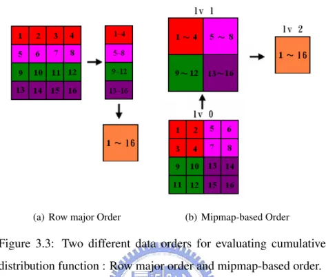
(37) 3.2 Implemetation on GPU. 26. u over the interval [0,1). The resulting samples are F −1 (u). This technique is illustrated in Figure 3.2.2.. Figure 3.2: Inverse CDF sampling [3]. When generating cumulative distribution function, the order of sequence can be arbitrary. In the case of two dimension space, the row major order is usually used. Figure 3.3(a) shows a row major order on 4x4 texture. The inverse result F −1 (u) can be derived by binary searching of the data structure. The row major can not fully utilize the features of GPU, texture structure and parallel computation. Therefore, we use mipmap-based order, as shown in Figure 3.3(b). The process of cumulation can be performed by mipmap construction of GPU. Inverse result F −1 (u) can be derived by traversing the mipmap structure from top level to the lowest level. In this stage, we first use mipmap construction to generate the cumulative distribution function F (x). Because the inverse process of each sample with associated u can be performed independently, we generate samples in pixel shader. We render an image which contains at least N pixels. Each pixel is assigned a value u which is generated uniformly over the interval [0,1). Then, N samples are generated according to the given distribution p(x). Just like previous stage, we render the information of samples into a 2D texture, as an input of final stage. The pseudo code of sampling is shown in Algorithm 3.1..

(38) 3.2 Implemetation on GPU. 27. (a) Row major Order. (b) Mipmap-based Order. Figure 3.3: Two different data orders for evaluating cumulative distribution function : Row major order and mipmap-based order. Evaluation of the translucency With information of samples, we can evaluate the radiance at each outgoing point of model surface. For each rendered pixel, we fetch all samples by 2D texture look up and sum up the contribution of translucency. The equation for computing outgoing radiance is shown below : − L(xo , → ωo ) = =. 1 − F (η, → ωo )B(xo ) π t → − 0 PN Ft (η,ωo )Eavg i=1 Nπ. (3.6) Rd (xi , xo ). − In Equation 3.6, the diffusion function Rd (xi , xo ) the Fresnel transmittance Ft (η, → ωo ) contain operation of trigonometric, square root, and exponential function, which are complicated instruction. In order to reduce the computation cost of integration, we store the function as a texture. According to the Equation 2.12, the diffusion function Rd (xi , xo ) can be represented as one dimension function about the distance between xi and xo . Rd (xi , xo ) = Rd (r) where r = |xo − xi | is the distance between the incident and the outgoing point..

(39) 3.2 Implemetation on GPU. 28. Therefore, we scale the diagonal length of input object to 1, and store the diffusion function Rd (r) as a one dimension texture with interval [0,1]. We do the same thing on Fresnel − transmittance Ft (η, → ωo ) by using dot product of normal and view direction as parameter. We transform the radiance to color using DirectX’s HDR Lighting, which is a tone mapping algorithm commonly used in real-time high dynamic range lighting. We approximate the aver0 age radiance Radavg of rendered pixels by the average irradiance Eavg computed at the second. stage. Therefore, we can integrate the tone mapping into the final stage without any additional pass. The equation for computing outgoing radiance is shown below : Radscale (x, y) = Color(x, y). =. Rad(x,y) Radavg 1+Radscale (x,y) Radscale (x,y). After tone mapping, we add specular effect by phong lighting and generate the final image..

(40) 3.2 Implemetation on GPU. 29. Algorithm 3.1: The algorithm of sampling by traverse mipmap structure. int LVmap = M; // Level number of mipmap (10 for 1024x1024) 0 float Eavg ;. // Average of irradiance function. float P;. // associated probability. vec2 loccurrent =vec2(0.5,0.5);. // Sample loc in current level. vec2 locnext ;. // Sample loc in next level. vec2 texelnext [4];. // four corresponding texel loc in next level. float Ij ,Inext =0.0;. // temporal variable. 0 P*= 4.0*Eavg ;. // Change probability to irradiance value. texelnext [0]=vec2(-0.5,-0.5);. texelnext [1]=vec2( 0.5,-0.5);. texelnext [2]=vec2( 0.5, 0.5);. texelnext [3]=vec2(-0.5, 0.5);. for(int i = LVmap -1 ; i ≥ 0 ; i–) { // Start from second level to lowest level for(int j=0;j<4;j++) { texelnext [j] /=2.0; // fetch irradiance of texel j in next level Ij = texture2DLod (loccurrent +texelnext [j],i); if( P > 0.0) { locnext = texelnext [j]; Inext = Ij ; P -= Ij ; } } loccurrent = loccurrent + locnext ; P += Inext; P *= 4.0; }.

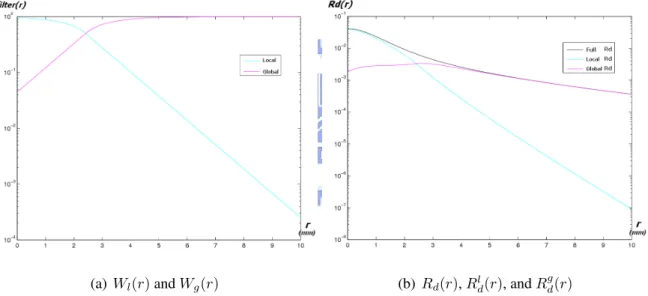
(41) 3.3 Hybrid Approach. 3.3. 30. Hybrid Approach. The diffusion term is the most costly to sample for translucent materials since it depends on lighting from a large fraction of the model surface. Jensen and Buhler [9] evaluated the integration by uniform sampling over the model surface. In order to generate accurate result image, the use the mean-free path `u as the maximum distance between neighboring samples. `u = 1/σt0 is the average distance at which the light is scattered. Therefore, the approximate number of points the used is A/(π(`2u ) for a given object. When σt0 of the material property or model size is large, the number needed for accurate result will be very high. In this case the appearance of translucency will be dominant to local effect. This problem also happens for our texture space importance sampling method. In order to overcome this problem, we decompose the integration equation into a local term and a global term. We apply our texture space importance sampling method on the global term. For the local term, we combine two run-time translucent method proposed by Mertens et al. [15], and by Dachsbacher and Stamminger [2].. 3.3.1. Separation of Diffusion Function. We decompose the diffusion function Rd(xi , xo ) into a local term and a global term by an exponential weighting function. The detail diffusion function is described in section 2.3. The weighting equation is shown below : Wl (r) = {. 1.0− 0.5e−(r−Rp )·K r ≤ Rp 0.5e−(r−Rp )·K r > Rp. ,. Wg (r) = 1.0 − Wl (r). where Rp is the position where the contributions of the global and local term are equal, and K is a constant. Therefore, the outgoing radiosity B(xo ) in Equation 2.13 can be reformulated as.

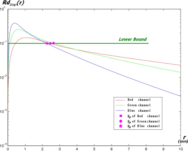
(42) 3.3 Hybrid Approach. 31. following : B(xo ) =. R. =. R. =. R. A A A. E(xi )Rd (xi , xo )dxi E(xi )Rd (r)(Wl (r) + Wg (r))dxi E(xi )Rd (r)Wl (r)dxi +. R A. .. E(xi )Rd (r)Wg (r)dxi. = Bl (xo ) + Bg (xo ) where r = |xo − xi | is the distance between the incident and outgoing point. Figure 3.4 show example of filter function, and divided diffusion function, Rdl (r) = Rd (r)Wl (r) and Rdg (r) = Rd (r)Wg (r). The extreme high value of short distance is retained in the local term, and the global term preserves the function value of far distance, as shown in Figure 3.4(b).. (a) Wl (r) and Wg (r). (b) Rd (r), Rdl (r), and Rdg (r). Figure 3.4: Graph of weighting function and diffusion function. Rp is 2.4141 and K is 1.5 for weighting function. σa is 0.0024, σs0 is 0.70, and η is 1.3 for diffusion equation (parameters of red channel for skimmilk [10]). The center of weighting function Rp is not easy to be assigned. The global term will still contain the distinct local effect if Rp is too small. If Rp is too large, the global term will leave for nothing. We develop an automatic way to assign Rp . We define an importance function by the product of diffusion and circumference of distance. RdImp (r) = Rd (r) ∗ 2πr..

(43) 3.3 Hybrid Approach. 32. We set a importance lower bound (10−1 in our experiment), and find the intersection with importance function. Rp is assigned to the largest intersection value. Figure 3.5 shows an example of importance function, importance lower bound, and Rp of color channels for Skimmilk. We apply our texture space importance sampling method on on local term and global, the result image is shown in Figure 3.6.. Figure 3.5: Graph of importance function for skimmilk material.. 3.3.2. Method for Local Translucency. Mertens et al. [15] and Dachsbacher and Stamminger [2] both proposed methods for computing translucent effects in run-time without precomputation. These two methods were developed.

(44) 3.3 Hybrid Approach. (a) Full. 33. (b) Local. (c) Global. Figure 3.6: Image with (a) Full Rd function, (b) Local Rd function, and (c) Global Rd function. Model is 10mm MaxPlanck and material is Skimmilk. based on a similar idea : evaluating the integration on projection plane. Mertens et al. render the irradiance map from the light view, similar to the concept of shadow map, and then evaluate integration by applying a fixed filter on the irradiance map, as shown in Figure 3.7. For each rendered pixel the filter is located at the center of projected location. Dachsbacher and Stamminger proposed another approach ”Efficient Rendering of Local Subsurface Scattering” [2]. They render irradiance map from the camera view and apply importance sampling on the projection plane for each pixel, as show in Figure 3.8. There is a problem for method proposed by Dachsbacher and Stamminger. They render irradiance map from camera view and evaluate the integration. If the camera turns to the other side of light source, there will be almost no irradiance caught by the map. Mertens et al. used a fixed filter with 21 samples in their method. Their method is not flexible enough to render all kinds of translucent materials in arbitrary size. Therefore, we propose to combine these two different methods. We render an irradiance map from light view, and designed a flexible filter based on the importance sampling strategy over projection plane in [2]. The integration of.

(45) 3.3 Hybrid Approach. (a). 34. (b). Figure 3.7: Translucent Shadow Map [15] : (a) Irradiance map rendered from light view. Figure 3.8: Overview of ”Efficient Render-. with filter. (b) A filter pattern with 21 sam-. ing of Local Subsurface Scattering” [2].. ples. radiosity B(xo ) in Equation 2.13 is reformulated as following : B(xo ) =. R. =. R. A P. E(xi )Rd (xi , xo )dxi E(xi )Rd (xi , xo )dxi 2 dxi. .. (3.7). Where P is the space of projection plane; And dxi is the corresponding depth of xi from light view; We generate N sample with associated area size over projection plane. Then, we can evaluate the integration as a summation of each sample. B(xo ) =. PN. =. PN. i=1. E(xi )Rd (xi , xo )A(xi )dxi 2. 0 i=1 E(xi )Rd (xi , xo )A (xi ). .. (3.8). where A(xi ) is the corresponding area for a sample on the projection plane, and A0 (xi ) = A(xi )dxi 2 . A(xi ) is fixed once we decide the sample pattern, but A0 (xi ) is adaptive according to the exact depth of a sample in run-time. We replace the fixed filter pattern with 21 samples in [15] for flexibility. We generate an circular sample pattern with LxC + 1 samples, as shown in Figure 3.9. L is the number of circles and C is the number of samples in each circle. The additional sample is the center of the filter. Samples in same circle will be uniformly distributed by angle. We determine the radii.

(46) 3.4 Discussion. 35. of each circle by using the importance sampling strategy on the projection plane proposed by Dachsbacher and Stamminger [2]. Therefore, we can evaluate the local with flexibility between performance and quality. We name this modified method ”Local Translucent Shadow Map”.. (a). (b). Figure 3.9: Our method for local translucency. (a) Irradiance map rendered from light view with filter. (b) Filter pattern with 17(4x4+1) samples.. 3.4. Discussion. Our hybrid method uses two difference concepts to render local and global translucent effects. Both methods convert the integration over model surface to integration over another space domain. One is 2D texture space and the other is 2D projection plane. Figure 3.10 shows the system overview of our hybrid method. The integration of local effects and global effects can be evaluated simultaneously in the same pass. Additional pass is needed to render the irradiance map to the projection plane from the light view..

(47) 3.4 Discussion. 36. Originally, we try to design a method to evaluate the local translucent effect on the texture space. Hence, we can compute the local and global effect over the same domain, texture space. The overview is shown in Figure 3.11. We develop another importance sampling strategy based on the diffusion function Rd(xi , xo ). We study the distribution of Rd(xi , xo ) on texture space for each outgoing point xo , and find out the situation is too complicated to analyze because of the stretch of angle and distance. We assume the texture space is isometric mapping, which means there is no stretch on the path of any two points. On the texture of isometric mapping, we can easily apply the importance sampling strategy to evaluate the integration of local effect, similar to the method proposed by Dachsbacher and Stamminger[2]. Unfortunately, parameterization of isometric mapping is only exist in theory. Current method for parameterization only minimize some kind of error stretch, like area preserving, angle preserving etc.., but can not eliminate the stretch. Therefore, we develop an adaptive sampling method on current texture to approximate the importance sampling on isometric mapping. For each rendered pixel, we start from the texture location of pixel and generate samples iteratively along one direction. Next sample is determined by the direction, distance, and stretch of current sample. This method did not work very well in our experiment. Stretch is independent for each triangle, and the difference of stretch may be vary large for adjacent triangles in some case. In our method of adaptive sampling, we only consider the information of current sample. Therefore, the change along the path of current sample and next sample can not be took into account, which makes significant errors appear,as shown in Figure 3.12. The difference of stretch make the path in three-dimensional model space to change direction when passing the boundary the triangle. Figure 3.13 shows an example of this problem sampling method for one point on the forehead of MaxPlanck. As you can see, the shape and direction of sampling is still circular because the path crosses few triangle at the beginning. When the distance between two samples is increased, the path is turning into another direction. The shape of sampling is not circular anymore..

(48) 3.4 Discussion. 37. In order to overcome this problem, extra information need to be take into account. This will force us to lose the advantage of GPU-based texture space importance, rendering translucent material with lower precomputation overhead. Therefore, we use another approach to evaluate the local effect of translucency..

(49) 3.4 Discussion. 38. Figure 3.10: System overview of our hybrid method. The local and global effect are computed over the projection space and the texture space respectively..

(50) 3.4 Discussion. 39. Figure 3.11: System overview of our ideal method. The local and global effect are both computed over the texture space..

(51) 3.4 Discussion. 40. (a). (b). Figure 3.12: Diagram of adaptive sampling method on (a) texture space and (b) model space. Red point is current sample; Blue point is next sample; Green points are intersection of path and boundary of triangle.. (a). (b). Figure 3.13: Result samples of adaptive sampling method on (a) texture space and (b) model space for one outgoing point at the forehead. The color in (b) is the visualization of diffusion function Rd(xi , xo ) for the outgoing point..

(52) CHAPTER. 4. Result. All experiments are performed on Intel core 2 due E6600 2.4GHz PC using NVIDIA Geforece 8800 GTX graphics hardware. Most of our models are scaled to 10 mm and rendered in 512 × 512 screen resolution using difference scattering parameters described in [10].. 4.1. GPU-based Texture Space Importance Sampling. Performance Table 4.1 and 4.2 show the performance of our texture space importance sampling method using a resolution of 1024 × 1024 for irradiance map with difference sample numbers. We decompose performance into two part, preprocessing and integration. Preprocessing includes rendering irradiance to texture and importance sampling. Integration include the final stage of run-time, evaluation of the translucency. Figure 4.1 shows three difference result image of our method. We compare our method with ”Efficient rendering of Local Subsurface Scattering” LSS [2] in performance. Table 4.3 and Table 4.4 shows the performance of LSS. The performance of. 41.

(53) 4.1 GPU-based Texture Space Importance Sampling. 42. preprocessing in our method and LSS are both around 6 ms to 7ms. The computation cost our of integration in LSS is about 8 ∼ 9 times of our method.. Model. Number. of. Samples. Triangle. 49. 100. 169. 256. 400. 900. 1600. 2500. Sphere(28K). 28560. 5.31. 5.29. 6.47. 5.20. 5.25. 5.14. 5.12. 5.60. CowHead. 2072. 5.34. 5.23. 4.86. 5.11. 5.16. 5.14. 4.86. 4.70. TexHead. 8924. 5.30. 5.26. 5.10. 5.31. 5.46. 5.42. 5.14. 4.59. MaxPlanck. 9951. 5.29. 5.11. 5.33. 5.19. 5.31. 5.29. 4.95. 4.65. Parasaur. 7685. 5.29. 5.43. 5.17. 5.52. 5.41. 5.71. 6.25. 6.15. Table 4.1: Performance of preprocessing in our method with difference model in millisecond (ms).. Model. Number. of. Samples. Triangle. 49. 100. 169. 256. 400. 900. 1600 2500. Sphere(28K). 28560. 448.6. 242.3. 179.7. 101.5. 65.9. 29.8. 16.5. 10.4. CowHead. 2072. 1123.0. 623.7. 393.3. 267.4. 177.3. 81.0. 45.1. 28.4. TexHead. 8924. 822.6. 448.5. 277.1. 187.5. 122.5. 55.7. 30.8. 19.4. MaxPlanck. 9951. 783.9. 430.1. 268.0. 180.5. 118.0. 53.4. 29.8. 18.7. Parasaur. 7685. 1069.9. 602.1. 377.5. 258.6. 168.3. 76.2. 42.9. 27.0. Table 4.2: Performance of integration in our method with difference model in frame per second (fps)..

(54) 4.1 GPU-based Texture Space Importance Sampling. 43. Figure 4.1: Result image using our method in Table 4.2. (a) MaxPlanck with skimmilk and 900 samples in 53.4 fps (b) Parasaur with skin1 and 1600 samples in 42.9 fps (c) TexHead with marble and 2500 samples in 19.4 fps.. Model. Number. of. Samples. Triangle. 49. 100. 169. 256. 400. 900. 1600 2500. TexHead. 8924. 6.27. 6.26. 6.12. 6.37. 6.51. 6.49. 6.73. 6.90. MaxPlanck. 9951. 6.16. 6.82. 6.95. 6.18. 6.42. 6.18. 5.46. 6.26. Parasaur. 7685. 5.93. 6.05. 6.04. 6.04. 6.12. 5.97. 5.86. 5.95. Table 4.3: Performance of preprocessing in LSS with difference model in millisecond (ms).. Model. Number. of. Samples. Triangle. 49. 100. 169. 256. 400. 900. 1600. 2500. TexHead. 8924. 108.6. 53.3. 30.7. 20.4. 13.2. 5.7. 3.2. 2.1. MaxPlanck. 9951. 100.2. 50.1. 29.1. 18.7. 11.9. 5.3. 2.9. 1.9. Parasaur. 7685. 145.8. 70.0. 41.3. 27.6. 17.4. 7.7. 4.3. 2.8. Table 4.4: Performance of integration in LSS with difference model in frame per second (fps)..

(55) 4.1 GPU-based Texture Space Importance Sampling. 44. Compare Quality to Real-Time Method We compare our result image to LSS and ”Local Translucent Shadow Map” (LTSM) which is described in section 3.3.2. Figure 4.2 shows image of 10mm MaxPlanck with marble material in difference views by three methods. Because Dachsbacher and Stamminger rendered the irradiance map from camera view, irradiance will be caught poorly when the camera turn to the other side of light source. ”Local Translucent Shadow Map” can both render local and global effects, but same noticeable error will occur at the boundary of shadow map, as shown in the second row of Figure 4.2.. Figure 4.2: Top row are rendered by our method using 1600 samples in 29.8 fps. Second row are rendered by LTSM using 1600 samples in 8.0 fps. Third row are rendered by LSS[2] under same condition in 2.9 fps..

(56) 4.1 GPU-based Texture Space Importance Sampling. 45. Compare Quality to Non-Real-Time Method We also compare our result image to non-real-time method proposed by Jensen and Buhler [9]. Figure 4.3 and 4.4 show 10 mm and 40 mm igea rendered by our method and non-realtime method with different materials. As you can see from image, our texture space importance sampling method can real-time render translucent materials which is almost no difference with non-real-time method.. (a) skin1 Ours. (b) skin1 Jensen. (c) skin2 Ours. (d) skin2 Jensen. Figure 4.3: Result image rendered by our method and by Jensen and Buhler [9] with 10mm igea.. (a) skin1 Ours. (b) skin1 Jensen. (c) skin2 Ours. (d) skin2 Jensen. Figure 4.4: Result image rendered by our method and by Jensen and Buhler [9] with 40mm igea. Our approach can render dynamic translucent material. Figure 4.5 shows examples of dynamic size from 10 mm to 70 mm. The dominate appearance of translucency changes from the global effects to the local effects with the model size..

(57) 4.1 GPU-based Texture Space Importance Sampling. 46. (a) skimmilk. (b) skin1. (c) skin2. Figure 4.5: Result image using our method with different model size. Model sizes are 10, 25, 40, 55, 70mm from left to right..