Calibration of Radar Beam Weighting Effect for
2-D Angular Imaging of VHF Atmospheric Radar
Using Multiple Beam Directions
#Jenn-Shyong Chen
1, Jun-ichi Furumoto
21 Department of Computer and Communication Engineering, Chienkuo Technology University
No. 1 Jieshou N Rd, Changhua City, Taiwan, [email protected]
2 Research Institute for Sustainable Humanosphere, Kyoto University
Uji, 611–0011, Japan, [email protected]
Abstract
An approach using multiple beam directions is proposed for VHF atmospheric radar to yield an effective weighting pattern of radar beam for 2-D angular imaging. Such obtained beam pattern is found to be adaptive to signal-to-noise ratio of data. A practical radar experiment was conducted to demonstrate the proposed approach.
Keywords : Beam Weighting Effect, Radar Imaging, VHF Atmospheric Radar
1. Introduction
Radar technique using multiple receivers is capable of detecting the direction of arrival (DOA) of signal sources. It is termed coherent radar imaging (CRI) [1] when used with the VHF atmospheric radar. The CRI technique is expected to recover the angular turbulent structure in the atmosphere with some advanced algorithms of signal analysis such as Capon’s method [2], and consequently, the DOAs of echo centers of the atmospheric structure can be estimated. However, the DOAs are usually biased owing to the weighting effect of radar beam pattern. Modification of DOAs with a simulated radar beam pattern usually leads to an unrealistic result. In view of this, a practical approach to mitigation of the radar beam weighting effect is pursued in this study.
2. Calibration Approach
The polar diagram of the backscatter power detected by VHF atmospheric radar can be written as exp(-sin2θ/sin2θ
s), where θ is zenithal angle and θs is an estimate of aspect sensitivity
(termed aspect angle). The effective power distribution as a function of θ can be regarded as the product of exp(-sin2θ/sin2θ
s) and the radar beam weighting function, exp(-sin2θ/sin2θo), in which θo
is the half beam width of a vertical radar beam [3].
For an off-vertical radar beam and a tilted layer or non-homogeneous angular distribution of scatterers, the polar diagram of the backscatter power may not center on zenith. Therefore, the effective power distribution along the line of the tilted radar beam can be expressed
⎥ ⎦ ⎤ ⎢ ⎣ ⎡ ⎥ ⎦ ⎤ ⎢ ⎣ ⎡ = s 2 2 Ts o 2 2 T sin ) sin -(sin -exp sin ) sin -(sin -exp ) P( θ θ θ θ θ θ θ (1)
where θT is the off-zenith angle of the radar beam direction and θTs is the center of the scattering
distribution. Eq. (1) is valid for θT and θo less than ~10o [3]. Then it gives the polar diagram of the
backscatter power: sin ) sin -(sin exp ) P( sin ) sin -(sin -exp ) A( o 2 2 T s 2 2 Ts ⎥ ⎦ ⎤ ⎢ ⎣ ⎡ = ⎥ ⎦ ⎤ ⎢ ⎣ ⎡ = θ θ θ θ θ θ θ θ (2)
CRI-obtained power distribution (or termed brightness distribution) is supposed to indicate P(θ). Based on this, A(θ) can be retrieved theoretically after a proper correction of P(θ) with a suitable value of θo. An estimate of θo is thus needed, as addressed in the following.
Considering two symmetrically tilted radar beams that are transmitted almost simultaneously, the CRI brightness distributions of the two oblique radar beams originate basically from the same A(θ). Therefore, the backscattered power distributions, A1(θ) and A2(θ), retrieved
from the two oblique radar beams are expected to be close. Such an expectation is valid especially around the zenith where the viewing regions of the two oblique radar beams overlap most greatly. Referring to [4], the following estimator can be used to calculate the difference between A1(θ) and
A2(θ) around the zenith:
∑ ⎥ ⎦ ⎤ ⎢ ⎣ ⎡ + = ∑ = Δ = = N 1 i 1 i i 2 i 2 i 1 N 1 i 1 i 2 i 2 i 2 i 1 ) ( A ) ( A 2 -) ( A ) ( A ) ( )A ( A )] ( A -) ( [A E θ θ θ θ θ θ θ θ (3)
where N is the number of the brightness values estimated around the zenith and along the line of the two oblique radar beams. Giving various values of θo in (2) will result in different values of ΔE.
In (3), ΔE=0 for A1(θ)=A2(θ); if A1(θ)≠A2(θ), however, ΔE>0 and ΔE usually gets larger as
the difference between A1(θ) and A2(θ) is larger. According to this, the value of θo which makes ΔE
smallest can be regarded as the optimal half beam width (termed effective beam width and denoted as θe hereafter). Such obtained θe varies with some parameters of echoes; especially the
signal-to-noise ratio (SNR).The relationship between θe and SNR is expected to vary with the off-zenith
angle of the two symmetrically tilted radar beams, which can be comprehended as follows. The traditionally used radar beam width, θo, is given by assuming a Gaussian-shaped angular intensity
distribution in the radar beam, which is only suitable for the angular region within ~θo. To give a
more accurate description of angular intensity distribution in the radar beam, different values of θo
are needed for different off-beam-direction angles if the Gaussian form is employed. The zenithal direction, where the effective beam width θe is estimated to represent the value of θo, corresponds to
different off-beam-direction angles for various oblique radar beams; hence the value of θe varies
with the off-zenith angle of the oblique radar beam. Consequently, the values of θe estimated from
various oblique radar beams can be used to take shape the radar beam weighting pattern.
3. Instrument and Radar Imaging
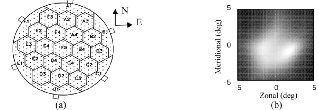
The above calibration approach was demonstrated by using the Middle and Upper (MU) atmosphere radar in Japan (34.85oN, 136.11oE; central frequency: 46.5 MHz). Fig. 1a shows the
antenna array configuration of the MU radar, in which A1~F5 indicate 25 antenna groups. These antenna groups can be combined arbitrarily for transmission and reception. In this study, full array was used for transmission, and nineteen antenna groups A2, A3, A4, B2, B3, B4, C2, C3, C4, D2, D3, D4, E2, E3, E4, F2, F3, F4, F5, were set for reception. Radar plus length was 1 μs and sampling time
step was also 1 μs, giving a range resolution of 150 m and a sampling height interval of 150 m, too. Radar beam was vertical. More characteristics and capabilities of the MU radar can refer to [5].
5 0 - 5 -5 0 5 Zonal (deg) −5 0 5 5 0 5 N E Meridional (d eg) (a) (b)
Figure 1: (a) MU VHF radar. The number of antennas (Yagi) is 475, and the radius of the array is ~55 m. A1 to F5 denote twenty five antenna groups. (b) Angular brightness distribution retrieved by Capon’s method. The brightness values are normalized and displayed in linear scale.
A variety of inversion algorithms can be employed to deal with multiple-channel signals/echoes; in this study the Capon method was employed [2], [6]. The Capon method is
time-saving and suitable for distributed target like refractivity irregularities in the atmosphere, which can be used with the CRI data in both time and Doppler frequency domains. In this study, the time-domain calculation was executed to estimate the so-called angular brightness brightness− P(θ) in (2). One example is shown in Fig. 1b, where two scattering centers were observed.
4. Calibration Results
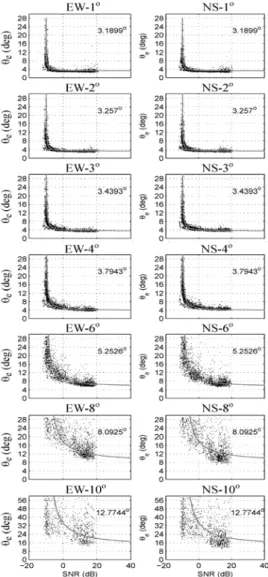
Fig. 2 shows the scatter diagram of θe versus SNR. As seen, θe approaches to some values
as SNR is getting large. On the other hand, θe increases dramatically as SNR is close to ~-10 dB.
Based on the feature in Fig. 2, it is possible to find a set of equations for fitting the relationship between θe and SNR at different off-beam-direction angles, as follows:
1) Give a set of θo for all beam pairs that can indicate the effective beam widths at infinite SNR.
Such a value set, denoted as θoe hereafter, can be assigned approximately by extending the
dependent relationship in Fig. 2 to very high SNR. For example, if the set of θoe=[2.80o, 3.00o,
3.50o, 4.00o, 5.50o, 8.50o, 12.50o] are given for the beam pairs tilted to the zenith angles of
θT=[1o, 2o, 3o, 4o, 6o, 8o, 10o], then a cubic curve,
2 3 T 1 oe
=
c
θ
+
c
θ
(4)is capable of depicting the relationship between θoe and θT. Fig. 3 shows the fitting result, with
the constants c1≒0.0096 and c2≒3.1803. Such obtained cubic equation can be employed to
estimate effective beam widths at infinite SNR for various off-beam-direction angles, by regarding the off-zenith angle θT as the off-beam-direction angle of a radar beam.
2) Substitute the value of θoe, estimated with (4) for an off-beam-direction angle (i.e., the variable
θT), into the following equation which describes the relationship between θe and SNR (in dB):
oe 4 2 3 e 10
θ
θ
θ
+ + + = SNR c c oe (5) where c3≒1.4751 and c4≒-9.7430 for the fitting curves shown in Fig. 2. Notice that c1−c4 areconstants resulting from fitting processes.
Eqs. (4) and (5) are empirical and they are not unique. In addition, in the use of (5) SNR must be larger than -10 dB to avoid a negative θe. In view of this, other expressions which can
describe the relationship between θe and SNR well can also be employed.
Fig. 4 exhibits two examples of original and modified CRI brightness distributions, presented with contour lines. As seen, the contour map corrected by a fixed beam width is unrealistic (Fig. 4(b)), which is of no use. By contrast, the contour map rectified with an adjustable beam width reveals some noticeable features (Fig. 4(c)): (1) in the left column, the raw contour map shows a double–center pattern, which also appears in the corrective map but with a larger separation between the two centers; (2) in the right column, the single echo center in the raw map changes to double echo centers. In view of this, correction of radar beam weighting effect on CRI brightness is indeed crucial sometimes; it may revise the number and locations of echo centers, the brightness width, and then reveal some concealed information in the radar echoes of the atmosphere. Extended works of the present study are: (1) validating the proposed approach for various radar parameters and atmospheric conditions; (2) applying the proposed approach to practical issues such as measurements of vertical wind and aspect sensitivity of the atmosphere.
References
[1] R. F. Woodman, “Coherent radar imaging: Signal processing and statistical properties,” Radio Sci., vol. 32, no. 6, pp. 2372–2391, doi:10.1029/97RS02017, 1997.
[2] J. Capon, “High-resolution frequency-wavenumber spectrum analysis,” Proc. IEEE, vol. 57, no. 8, pp. 1408-1418, 1969.
[3] W. K. Hocking, R. Rüster, P. Chechowsky, “Absolute reflectivities and aspect sensitivities of VHF radio wave scatterers measured with the SOUSY radar,” J. Atmos. Terr. Phys., vol. 48, pp. 131–144, 1986.
[4] J.-S. Chen, M. Zecha, “Multiple-frequency range imaging using the OSWIN VHF radar: Phase calibration and first results,” Radio Sci., vol. 44, no. 1, RS1010, doi:10.1029/2008RS003916, 2009.
[5] G. Hassenpflug, M. Yamamoto, H. Luce, S. Fukao, “Description and demonstration of the new Middle and Upper atmosphere Radar imaging system: 1-D, 2-D and 3-D imaging of troposphere and stratosphere,” Radio Sci., vol. 43, RS2013, doi:10.1029/2006RS003603, 2008. [6] R. D. Palmer, S. Gopalam, T.-Y. Yu, S. Fukao, “Coherent radar imaging using Capon’s
method,” Radio Sci., vol. 33, no. 6, pp. 1585-1598, doi:10.1029/98RS02200, 1998.
Acknowledgments
This study was supported by the National Science Council of ROC (Taiwan) through grants NSC98-2111-M-270-001 and NSC99-2111-M-270-001-MY2.
Figure 3: Relationship between effective beam width and off-zenith angle of the radar beam direction for the condition of infinite SNR. The fitting curve results from (4).
Figure 4: Contoured CRI brightness distribution (self-normalized): (a) original, (b) modified with the half beam width of 3.46o,
and (c) modified with adaptable beam width. Plus sign indicates the mean location of echo center. Contour levels are ten.
Figure 2: Scatter diagram of effective beam width (θe) versus signal-to-noise ratio (SNR).
The curves result from (5). The value given in each panel is the effective beam width estimated with (4) for the condition of infinite SNR.