2004 IEEE International Conference on Systems, Man and Cybernetics
A Tabu Search Algorithm for Satellite Imaging
Scheduling*
Wei-Chen Lin
Department
of
Electrical Engineering National Taiwan UniversityTaipei,
106,
TAIWAN
[email protected]Abstract
-
This paper deals with the daily imaging scheduling problem f o r a low-orbit, earth observation satellite, which belongs f a a class of single-machine scheduling problems. Its salient features includesequence-dependent setup effects, job-assembly
characteristics, and time window constraints. Instead of looking for the global optimal solutions, we adopt a promising evolutionary approach. Tabu Search. to solve
this scheduling problem. Numerical results demonsbwte that the approach is effective and efficient in applications to the realproblems.
Keywords: Satellite Scheduling, Tabu Search
1
Introduction
This paper deals with the daily imaging scheduling problem for a low-orbit, earth observation satellite, ROCSAT-I1 [9]. The daily imaging scheduling problem considers various imaging requests with different reward opportunities, changeover efforts between two consecutive imaging tasks, cloud coverage effects, and the resource availability of the spacecraft. It belongs to a class of single-machine scheduling problems with salient features of sequence-dependent setup times, job-assembly, and the constraint of operating time windows.
The ROCSAT-I1 daily imaging scheduling problem is NP-hard in computational complexity [ 5 ] . For problems of such high complexity, dynamic programming and exhaustive search techniques are either too time- consuming
or
impracticalfor
optimal solutions. Rule- basedor
heuristic approaches can reduce the computation time drastically but the resultant optimality is not guaranteed. Mathematical programming approaches, such as Lagrangian relaxation [4], have the advantage of computational efficiency when the optimization problems are decomposable. In many cases, the computational times increase almost linearly with the problem size. However, a heuristic is usually needed to modify the dual solution into a feasible solution. Tabu search [l] is a meta-heuristic designed for tackling hard combinatorial optimizations problems. Contrary to random searchDa-Yin Liao
Department
of
Information ManagementNational Chi-Nan
University Puli, Nantou, 545, T A I W A Napproaches such as simulated annealing (SA) where randomness is extensively used, Tabu search is based on intelligent searching to embrace more systematic guidance of adaptive memory and leaming.
The daily imaging scheduling problem
of
an earth observation satellite involves dispatching a set of imaging tasks to cameras on the satellite. Verfaillie et al. [8] considered this problem as a valued constraint satisfaction problem and solved by a Russian doll search (RDS)algorithm. Tounsi and David [6] modified the algorithm with the idea of successive search method. Experiment results show that their algorithm improves the performance by 11% over the traditional algorithm.
Vasquez and Hao [7] formulated the daily imaging scheduling problem of SPOT 5 [lo] as a generalized version of the multi-dimensional knapsack model including a large number of binary and ternary logical constraints. They proposed a Tabu search algorithm by integrating important features of a neighbourhood, dynamic Tabu tenure mechanism, techniques for constraints handling, intensification, and diversification to
determine which photographs to be taken.
Lin et a1 [2], [3] adopted the Lagrangian relaxation and snbgradient optimization technique to solve the daily imaging scheduling problem of ROCSAT-11. Based on the dual solution, a greedy heuristic is developed to re- allocate imaging tasks to a feasible schedule. This greedy heuristic is quick and easy to implement. However, it could probably be trapped in a local optimum. Intelligent search techniques such as Tabu search can help escape from the local optimal trap.
In this paper, we adopt the Tabu search approach to generate a sound satellite imaging schedule within allowable computation time. Our Tabu search algorithm consists of three Tabu steps: exploration, intensification, and diversification, which use the same Tabu-search- engine. Figure 1 shows the framework of our Tabu search algorithm.
lw!,wF] : opportunity window of task i, w: and w; are
<(I) ~dedls Aj
Bi
the time frame available for processing task i; : suitability of task i at time I ;
: penalty of incompleteness ofjob j , Ai 2 0 ; : suitability benefit of task i, B. t 0 ;
s m m
: *
-
i
l.--r---'---
'
T
-m
:
L....
L
---
1 [wt,wn.] :the nth cloud coverage area, n=l,...8
Exploration is the basis of the Tabu search algorithm. It explores efticiently and extensively over constraint- related search spaces. The results include the kernel schedule, defined as the best schedule found within exploration step, and the flipping information of decision variables. These results are then used to create the search spaces for intensification and diversification steps.
Intensification focuses on the search to exploit regions of the space that the search history suggests to be promising. On the other hand, diversification undertakes to explore regions that differ from regions previously visited.
In
our algorithm, intensification forces the search to exploit exclusively the areas around the kernel schedule. Diversification drives the search to explore areas that are either new or not frequently visited.The remainder of this paper is organized as follows. Section 2 presents the ROCSAT-I1 daily imaging scheduling problem formulation. Solution methodology is described in Section 3. Section 4 conducts the numerical experiments and demonstrates its ability in the applications to ROCSAT-II imaging scheduling. Finally, in Section 5 concluding remarks are made.
2
ROCSAT-I1 Imaging Schedulingg
Let us define some notations before modeling the satellite imaging scheduling problem.
Notations
T : scheduling time horizon; I
J
i
:job index,jcJandJ=IJI;4
I
: time period index, + l , . . , , T ; : collection of imaging job requests; : collection of tasks o f j o b j ; : collection of all tasks, I =
U
Ii ;i d i, k Pi ck? S!d M D
: task index, i, k d and I=lA;
: imaging (processing) time of task i;
: unit cost of setup from processing tasks k to i; : setup time from processing tasks k to i; : image storage capacity of Solid State Recorder;
: available power before the imaging operations : imaging mode of task i, mi E {Panchromatic
: image size of task i;
: power required for processing task
i;
: power required for setup from task k to i ; begin;
(PAN), Multi-Spectral (MS), PAN+MS);
a,, : a step function indicating that task
i
is 1, 'dt 2 hi;0, 'dt < h i ;
processed, where ai, =
P,
: a binary variable indicating job j is complete, 0, if +I) = 1, V i c I j ; where pj ={
, otherwise;
YE, : decision variable for setup from processing l , V t > h j - s k i ;
0, otherwise; tasks k to i, where ykit =
Define a task to be a basic operation of image acquisition over an area of the earth. Since an imaging request may need more than one tasks, let a job be the collection of all the tasks to fulfill the request. Some assumptions are made as follows.
I . 2. 3.
4.
A task can belong to a job only and can only be processed at most once during the time horizon. Only a task is processed or Setup at a time.
All the imaging requests are released and given at the beginning of the scheduling time horizon.
There are N distinct areas with cloud coverage above them during the scheduling time horizon.
Initial Setup Constraint: Assume that the initial state of
the satellite
is
setup to a dummy task, 0, where, sot = 0 , CO, = 0 , and vo, = 0 , vi E I.
As there is one and only onetask that can be setup from task 0, we have
Seruu Constraints: An imaging operation cannot commence its processing before completing its setup. We have
I 1=0
I i r
a,,
=IYII(,-$k,)3
'di, 1. (2) Machine Cauacitv Constraints: Since there is only onecamera equipped with the satellite, at any time, there is at most one task being processed or setup on the satellite, that is,
Storape Caoacitv Conslraint: The images acquired are
a ground station. As the total available memory on board is limited, this may impose constraints on the selection of images as well as their scheduling. The total size of images taken should be less than the available image storage capacity before imaging operations take place.
(4)
Power Consumption Construin/: The total power
consumption for imaging and setup operations should he less than the available power,
D.
Window of Cloud Coveruee: The mission of ROCSAT-I1 is to acquire substantially cloud-free images. We accomplish this by employing cloud coverage prediction data sets from the weather forecast data from Central Weather Bureau (CWB). Any task that intends to take images of a cloud-covered area is considered invalid.
b , a [ w ~ - p , , w ~ j V i , n = l , . . _ , N . (6) Binary Cons/ruints: As the variables a,
fi,
and y are all of either 0's or l's, the following binary constraints should be satistied.a , ~ { 0 , 1 } , V ~ E I J . (7-1)
Pj
E {0,1},Yi
E J . (7-2) Yki, E(0,1}, V k , i E I , t . (7-3) The objective of our satellite imaging scheduling problem has three folds: (i) to minimize the weighted number of incomplete jobs, (ii) to maximize the suitability benefits of imaging within the window of opportunity, and (iii) to minimize the total setup costs incurred. Mathematically, it is formulated assubject to constraints (1) to (7).
In (P), the first term is for the weighted number of incomplete jobs, the second for preferences of placements within the window of opportunity, and the third for the costs incurred by setup operations. For tackling the job- assembly effects, the weighted number of incomplete jobs is decoupling into the weighted number of incomplete tasks. Hence, a new mathematical formulation is defined as (P'), which serves as a lower bound of (P) and is solved by our Tabu search algorithm.
. . .
subject to constraints (1) to (7),
3 Tabu Search Scheduling
'3.1 Unconstrained and Constrained Search Space Define the unconstrained search space S to be composed of all binary vectors of I elements, where S = { ( a j , , a z r ,
. .
.,
a ,
) E {O,ly ). Note that the size of S maybe huge for large number of I. Moreover, a solution has to satisfy all the constraints. Denote C he the constrained
search space that is composed of all binary vectors of
I
elements, satisfying the initial setup constraint, setup constraints, machine capacity constraints, and windows of cloud coverage, i.e.,
C= {s E S
I
s satisfies constraints ( I ) to (3), (6), and (7)). Vasquez and Hao [7] indicate that high quality sub- optimal solutions are located at the frontier of feasibility. Often these solutions are difficult to reach uniquely from the feasible side. A more effective way is to allow the search to oscillate around the feasibility frontier, increasing the chance to reach good solutions. Hence, we relax the constraints of storage capacity (3) and power consumption (4) to accelerate the search.3.2 Neighborhood and Move
Define neighborhood function N: C + (2'-0) as follows. Let s=(alr.a2
,,...,
~ , , ) E c . s'=(a;,,a;,,.__,
a;,) is a neighbour of s, i.e. s' E N ( s ) , if and only if the followingconditions are satisfied ( I ) There exists one and only one task i such that U, = O and a;, = I ( I s i i I ) ; and (2)
sf =(a;,&
,...,
a;,).c.
Thus, s' can be obtained by adding an imaging task, say a,,, into s and at the same time removing some tasks from s to maintain the feasibility of the resultant schedule
SI. Let mv(i)=
(a,,
: O + 1)U (akr : 1+
~ , k E~ , k
# i )denote such a move. The number of possible moves from a schedule s equals the number of variables in s with its
value equal to 0. N(s)
has exactly IZI neighbouring schedules.
From the definition of decision variable a , , the switch of its value from 0 to 1 represents not only which image but also determine the time to take the image.
3.3 Tabu List Management
A Tabu list Tis to prevent the search from short-term cycling. For example, 1
+
0+
1+
0+.
.
.
, Each timewhen a move mv(i)= (ai, : 0
+
1) U (a& : 1+
O,k E I , k # i ) carries out, the moves m v ( j ) = ( a j , : O + I ) and mv(k)= (ab : 0+
1) will be the classified Tabu for some following iterations (Tabu tenure) to avoid resetting the values of aj, and a , from 0 to 1. The number of iterations, iterfin). during which a move mv(ni). m = j , k, is the classified Tabu is dynamically defined as below [ 6 ] .iter(m) = a x freq(m), a is a constant
where freq(m) is the number of times that a,,,, has been flipped from 1 to 0 from the beginning of the search. Therefore, the Tabu tenure of a move depends on the flipping frequency of the decision variable, which is to
penalize a move that repeats too often.
In order to implement the Tabu list, a vector @ of I
elements is used. ’ Each element @(i) (1
<
i 5 I ) records thesum of i m ( i ) and the cument number of iterations. In this way, it is very easy to know if a move mv(i) is a Tabu or not at iteration 1. If @(i) > I, in$;) is a forbidden move; otherwise, mv(i) is a possible move.
3.4 Resolution of Constraint Violation
1.2.1 1-0 be the set of indices of ker‘ that are equal to 0 and 1-1 those equal to 1.
1.2.2 I c_ L O contains the indices of elements where flipping of these elements does not affect the elements of Ll even after repairing the constraint violations.
1.2.3 D collects the indices of elements having a flipping frequency lower than the average. 1 . 3 1 - 0 , s c k e r ‘
2.1 Call Tabu-Search-Engine with I Step 2: // Intensification
2.2 I t 0 , s - (0,O ,..., 0) Step 3: //Diversification
3.1 Call Tabu-Search-Engine with D
3.2 I t 0 , k e r * c (0,O
,...,
0 ) , s c best solution found from step 3.13.3 c o u n f t counr+l
// end of while Step 4: // Output s*.
if (not ‘$ai, = = I, I 5 i 5 I within s*)
else
// end of if
then do output << “the schedule is infeasible” do output << “the schedule is feasible”
Tabu-Search-Engine Step 0 //Assumption
0.1 Lets and s* be respectively the current and the best schedules.
During the iterative searching in Tabu-Search-Engine, 0.2 krc 0 , j r e q t {O,O,.’..,O) 0.3
Step 1: //Searching
Let ni(s) be the set of candidate moves from s
the storage capacity constraint (3) and power consumption constraint (4) are relaxed. That is, after the searching the neighborhoods of current schedule s, the storage capacity and power consumption constraints may be violated by the resultant schedule. Each time when there is any
(%f(s) induces a particular search space C I, or 0). while there are possible moves exist in N ( s )
1.1 Compute the best move mv(i) (break ties randomly).
// m<i) c arg ,m!n
&),
f(*): primal function. constraint violation, the scheduled task is removed to r a h ( r )minimize the cost and a new setup relationship is then built. Continue this step until no relaxed constraint is violated.
3.5 Tabu Search Imaging Scheduling Algorithm The stopping criterion is defined by a maximum number of iterations allowed. It is proportional to the problem size. Each Tabu step is triggered and stops automatically by the Tabu list management, whenever no more moves are admissible. The Tabu search algorithm is given below.
Tabu Search Imaging Scheduling Algorithm (TSISA) Step 0: //Initialization
0.1
0.2 counr c 0 // Iteration number IC 0 Le?-*, s, and s a t {O,O,
.
.., 0) //Initialize the Tabu list, k e P , s, and s*nhlle coum < count-mar Step 1: //Exploration
1.1 Call Tabu-Search-Engine with
c
1.2 Compute I, D with freq and ker’
1.2 s t s+mv(i), P . e q ( i ) t t , I c I
U
( m v ( i ) ) , 1.3 // Resolve the violations on storage capacityconstraint and power consumption constraint (for Exploration and Intensification).
while there is any relaxed constraint violation
1.3.1 Remove task i* from s, where i* is the index of ker c ker U s
ai.( E s and s e arg man [ f ( s ) - f ( s \
(pi.,})].
1.3.2 Adjust setups among the remaining tasks i n s
// end of while
1.3.3 if /[s)< f ( s * ) then s* t s ll end
of
while4
Numerical
Experiments
Numerical experimentation is conducted
to
assess the performance of the proposed satellite daily imaging scheduling algorithm. Features of job assembly, setup effects, cloud coverage, and opportunity windows are considered in the test cases. The algorithm is first tested with a projected ROCSAT-I1 daily imaging scenario to demonstrate its applicability to the realistic problem.Algorithmic properties of both computational efficiency and optimality are further explored with respect to job- assembly, setup effects, and time window constraints, respectively. In order to demonstrate the efficiency and effectiveness
of
our approach, the scheduling algorithm based on Lagrangian relaxation approach [2], [3] is adopted as the comparative algorithm.We implement both the Tabu search and Lagrangian relaxation algorithms in C language. All the experiments are conducted in a PC with dual INTEL Xeon-2.4GHz CPUs with 1 GB memory.
4.1 ROCSAT-11 Daily Imaging Scheduling
Consider a test scenario of the daily imaging scheduling problem of ROCSAT-XI. As shown in Fig. 2, there are five imaging jobs, Jobs 1-5, which are composed of nine tasks. These five imaging jobs consider the conditions of wide-spread tasks (Job I), large-area tasks (Job 2 ) , separate-but-in-a-same-strip tasks (Job 3), cross-stripped tasks (Job 4), and consecutive tasks (Job S), respectively. The time window of each task is determined by the geographical limitation of the task. The setup time between any two tasks is proportional to their geographical distance, and the setup cost is twice the value of the corresponding setup time. The parameters and coefficients o f the cost functions are listed in TABLE 1. The scheduling time horizon is of 100 time periods. Two cloud coverage areas areassumed with totally 4 time periods of invalid imaging operations.
I ,
I
114 116 118 120 122 124 126
Longitude (deg E)
Fig. 2 . A Projected Case (Source: NSPO) Define imaging loading as the ratio of total processing times over the scheduling horizon. Three test cases of light, heavy and overloaded imaging loads are designed. The required imaging time is 67 time periods for the light- loaded case, 80 for the heavy-loaded case, and 93 for the overloaded one.
TABLE 1 . 5 JOBS, 9 TASKS IN 100 TIME PEMODS
%ti-t.*
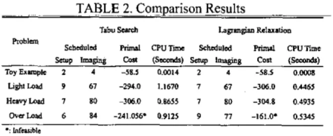
Numerical results of these three test cases are summarized in TABLE 2. The proposed Tabu search approach gets sound schedules for light and heavy loading cases, respectively. No feasible schedule is obtained for the overloaded case. TABLE 2 also shows the comparison results of both our proposed approach and the Lagrangian relaxation approach. Note that the proposed Tabu search approach is superior to Lagrangian relaxation approach in optimality but with little increase in computation time.
~~ ~ . ~~~~ TABLE ~~~~~~ 2. Comparison Results
T.bu sumh bp&C Rl1U.ti.m Srbcdulcd PMVl CPUTmX khdulcd m CPUame Roblen UgNlOld 9 67 -2s.O 1.1670 7 67 -306.0 0.4461 H I W W 7 80 -306.0 9.8655 I SO - 3 0 4 8 0.4931 "bid 6 84 -241.016. 0.9IZ5 9 17 -161.0. 0.535 *: hka.,bk 4.2 Algorithmic Features
In order to further explore the algorithmic features of our satellite daily imaging scheduling algorithm, 19 test cases are designed and simulated. All the test data are based on a realistic problem (case No. 5 in TABLE 3) as their baseline data set. The baseline problem considers 25 imaging jobs (J = 25) with 100 tasks (I = 100) to be scheduled within a time frame of 600 seconds
(T
= 600) when the satellite traverses the vicinity of the target area. The setup time and cost between any two consecutive tasks are randomly generated with mean setup time and variance to he one second, respectively. For each imaging task, its opportunity window, suitability function, and imaging mode are all randomly generated. The imaging size and power consumption factors of each task are assumed to he identical. They are 1 for PAN, 1.5 for MS, and 2 for PAN+MS. The power required to setup from taskk
to taski,
is set to he v b = l.Oxsb, V k, i. For all cases, their corresponding coefficients in the objective function are set to A, = 150, V j , B, = 15, V i, andCS
=2.0xsk,, V
k,
i. Each test case is simulated with 10 scenarios randomly. The loading of each test case is set to 66.7%. Simulation results are summarized in TABLE 3.The results
of
GroupI
indicate that there are no significant differences in optimality for different numbers of jobs. Also, the number of jobs has no impacts on the computational time. We therefore conclude that number of jobs has no direct impacts on both the optimality and the computational time. In order to study the setup effects on the satellite scheduling algorithm, five test cases are designed in Group 11. Results indicate that the costs become worse and the computational times become larger as the increase of setup times. The effects due to different lengths of time windows are designed and studied in Group 111. Note that the average costs become worse when the lengths of time windows decrease. However, the impact of computational time is not significant.In summary, most of the CPU times spent in the regular cases (in the same size of the baseline problem) are less than 385 seconds. The costs in most of the test cases are less than those of the Lagrangian relaxation approach. Therefore, we conclude that this daily imaging scheduling algorithm is quite efficient for realistic applications to provide a sound imaging schedule to the earth observation satellite.
5
Conclusions
This paper presents the development of a daily imaging scheduling system of an earth observation satellite, ROCSAT-11. The daily imaging scheduling problem of satellite belongs to single machine scheduling problems with salient features of sequence-dependent setup, job-assembly, and constrained operating time windows. It is formulated as an integer programming problem, which is NP-hard in computational complexity. We have developed an effective Tabu search algorithm to solve this problem. This Tabu search algorithm combines some ideas to make the searching effective and efficient. Those ideas include constrained neighborhood searching, greedy-based flipping process, and frequency-based dynamic Tabu tenure. Intensification and diversification
steps are used to avoid of being trapped in local optimum. Numerical results on three test scenarios of the daily imaging scheduling problem of ROCSAT-I1 and 19 realistic problems have shown the effectiveness of this algorithm. Comparison results also show our algorithm is superior to the Lagrangian relaxation approach in optimality but with little increase of computational time.
Future research may extend the algorithm to include realistic issues such as seasonal refreshment and coordination between multiple satellites. On the other hand, the developed algorithm deals with the scheduling problem assuming no machine failure and exclusions of imaging with cloud coverage. Extensions to this research may handle these stochastic issues.
References
[I] F. Glover and M. Laguna, Tabu Search, Kluwer Academic
Publishers, 1997.
[2] W:C. Lin, D:Y. Liao, C:Y. Liu, and Y:Y. Lee, “Daily Imaging Scheduling of An Earth Observation Satellite,” lEEE lnfernalional Conference on Siweiiis, Man, and
Cybernefics, Vol. 2, pp. 1886-1891,2003.
[3] W:C. Lin, D.-Y. Liao, C:Y. Liu, and Y:Y. Lee, “Daily Imaging Scheduling of An Earth Observation Satellite,” to amear in
..
IEEE Transaclio~ts on Sixlems, Man, andCybernetics, 2004.
141 P. B. Luh and D. J. Hoitomt. “Schedulin~ of Manufacturine
.1
-
-
Systems Using the Lagrangian Relaxation Technique,” IEEE Trans. on Aufomaric Corsfrol, Vol. 38, No. 7, pp. 1066-1079, 1993.
[SI M. Pinedo, Scheduling Theog,, Algon‘lhms, and Sj~sfms-2nd
Edifion, Prentice Hall 2002.
[6] M. Tounsi and P. David, “Successive Search Method for Valued Constraint Satisfaction and Optimization Problems,”
Proceedings o/rhe 13fh Infernarionol Conference on Took
w,ifh Arfi~~iallnlelligence, pp. 341-347, 7-9 Nov. 2001. [7] M. Vasquez and J. K. Hao, “A Logic-Constrained Knapsack
Formulation and . A Tabu Algorithm for the Daily Photograph Scheduling of An Earth Observation Satellite,”
Conipk&nal Opfim$aafion andAjy1icafions 20, No. 2, pp.
137-157.2001.
[8] G. Verfaillie, M. Lemaitre, and T. Schiex, “Russian Doll Search for Solving Constraint Optimization Problems,” In M I - 9 6 , Portland, Oregon, USA, 1996.
[9] NSPO: htm:ll~~~..nsno.eov.hv/.
[IO] Spot Image Spot 5 :
l~ttn:lluuu..sno~imaee.fr~o~nelsvste~~ future1 svot5lwelcome.htm.