A genetic algorithm approach for set covering problems

(1)

A

Genetic Algorithm Approach

for

Set Covering Problems

Wen-Chih

H u n g

,

Cheng-Yan

Kao+ and

Jorng-Tzong Horng*

Department of Computer Science and Information

Engineering

National

Taiwan University, Taipei, Taiwan

*National Central University, Chungli, Taiwan

+ All correspondences should be sent t o the second author.

Abstract

In this paper, we introduce a genetic algorithm approach for set covering problems. Since the set covering problems are constrained optimization problems we utilize a new penalty function t o handle the constraints. In addition, we propose a mutation operator which can approach the optima from

both sides of feasible/infeasible borders. We experiment with our genetic algorithm t o solve several instances of computationally difficult set covering problems that arise from computing the l-width of the incidence matrix of Steiner triple systems. We have found better solutions than the currently best- known solutions for two large test problems.

1 Introduction

Set Covering Problems (SCPs) [5] are difficult zero- one optimization problems. They are often encountered in a wide area of applications such as resource allocation [12] and scheduling [l, 21.

Fulkerson et al. [5] have given two empirically difficult set covering problems arising from S teiner triple systems. F'ulkerson et al. suggest that these are good problems for evaluating the computational efficiency of integer programming and set covering algorithms because they have far fewer variables than numerous solved problems in literature; however, experience shows that they are hard t o com- pute and verify.

The @-width of a (0,l)-matrix A is the minimum number of columns that can be selected from A such that all row sums of the resulting submatrix of

A are

at least

p.

Here /3 is an integer parameter ranging from zero t o the smallest row sum of the matrix A.

The l-width of A is:

w ( A ) = mineTz

subject to Ax 2 e,, ₍₁₎

z E (0, 1 Y ,

where e,, is an n-vector of ones and e,,, an m-vector of ones. The l-width is a set covering problem. The incidence matrix A that arises from Steiner triple systems has precisely 3 ones in each row. This matrix is also characterized as follow: for every pair of columns j and IC there is exactly one row

i

for which aij = a;k = 1. The incidence matrix of Steiner triple systems can be constructed by a recursive formulation 151.

computational experience with Ag, A15, A27 and

A45. They are able t o solve A9 with a cutting plane code after generating 44 cuts, but this cutting plane method is unsuccessful on the three larger problems. In contrast, using an implicit enumeration algorithm similar t o one developed by Geoffrion [6], they are able t o solve A15 and by further inspecting

the optimal solution, A27 can be solved in reason- able computer time. But several attempts at solving the problem A45 fail. Table 1 summarizes sev-

eral instances of the Steiner triple systems, showing that the sizes of optimal covers are known for few of them.

F'ulkerson, Nemhauser and Trotter [5] d' lSCUSS

2 Related Works

Karmarkar [8] gives an interior-point approach to solving 0-1 integer programming problems. Such problems, which are NP-complete in general, are converted t o nonconvex quadratic programs over polytopes. He experiments with the Steiner triple systems using his approach in [9] and produces the best known covers for all test instances. Because of nonconvex programming, some local optima

may be encountered during solution and the effect caused by the local optima becomes much more se- rious as the problem size is larger. This fact can be found from his result that his approach takes only about 6 minutes for problem As1 while over 56 hours and 226 hours for problems A135 and A243

(2)

respectively.

Fe0 and Resende [4] pursue a non-deterministic method for solving the difficult Steiner triple systems. The procedure is based on Chvatal’s itera- tive cost t o benefit greedy approach [3]. In order to improve upon ChvStal’s heuristic they introduce randomization. This heuristic also provides the best known solutions to all instances attempted in literature. However, our results are better than those of Fe0 and Resende.

Liepins et al. [IO, 111 investigate genetic algo- rithms for set covering problems with two types

of crossover operators in conjunction with three penalty functions and two multi-objective formulations. They do not experiment on the Steiner triple systems. Their results are encouraging and point to the greedy crossower, tight upper bounds for cost of completion of covers (as a penalty function P 3 ) , and Pareto based selection of the gene pool as promising techniques.

3 A

G A for Set Covering Prob-

lems

Genetic Algorithms (GAS) are search and optimization algorithms based on the mechanics of natural selection and natural genetics. The genetic search proceeds over a number of generations. “Survival of the fittest” provides the pressure for populations t o develop increasingly fit individuals. The primary monograph on the topic is Holland’s [7] Adaptation in Natural and Artificial Systems. Having been es-

tablished as a valid approach t o problems requiring efficient and effective search, genetic algorithms are now finding more widespread applications in busi- ness, scientific, and engineering.

In order to apply GAS to a particular problem, we first need t o select an internal string representa- tion for the solution space. Set covering problems seem to have a highly desirable string representa- tion, namely, binary strings of length N in which

the j - t h bit represents whether the j - t h set Pj is in the cover or not. Further implementation of our approach is described below.

Selection Strategy

The purpose of selection in a genetic algorithm is to give more reproductive chances to those population members that are better fit. Our mechanism for selective pressure is the linear function described

by Whitley [15].

index = POPULATION-SIZE x

(bias - sqrt(bias x bias - 4.O(bias - 1 ) x random()))

/2.0/(bias - 1 ) .

( 2 )

where the function random() returns a random frac- tion between 0 and 1. A bias of 1.5 implies that the top ranked individual in the population is 1.5 times more likely to reproduce (on one reproductive cycle) than the median individual in the population. Crossover Operator

Instead of Liepins’ greedy crossover we adopt the uniform crossover operator proposed by Syswerda [14]. Syswerda suggests that the probability of 1’s in the mask string be 0.5. But we find that probability of 0.6 results in better performance for our algorithms. This probability is fixed for all trials. Penalty Function

Richardson et al. [13] suggest that the penalty func- tion approach is the most suitable approach for constrained optimization problems such a.s set covering problems. Their illustration also convinces us that the infeasible solutions should provide information and not just be thrown away, especially the “next- door neighbors” of the optima in Hamming space. In view of this, we define a new penalty function P3’ as follows:

Let A be the incidence matrix of the original set covering problem with columns p j and associated costs cj.

P3’:

If S is a cover, then cost = c c j . If S fails to be a cover, then

JES

1. Set S‘ to S. Set total-cost to 0.

2. Strike each column, say p’, in S’ and the rows covered by p1 from A. Add the cost associated with p’ to the total-cost. Let

this new matrix be A’ and set A to A’.

3. For the unused columns and uncov- ered rows, calculate the cost-ratios (cost

1

number-of-rows-uncovered = cj num- be r-o f-ro ws-un col iered)

.

4. Append to S’ the column, say p 2 , with the least cost-ratio (break ties ran- domly). Add the cost associated with

p 2 to the total-cost.

5. Strike column p 2 and the rows covered by p 2 from A. Let this new matrix be

(3)

6. If S' is a cover, return total-cost as the cost of S. Otherwise set A to A' and go to step 3.

We note that P3' is more complex than P3 and proceeds in a column-by-column manner instead of the row-by-row manner of P3. This column-by-column manner can estimate the Hamming distance from the optimum more accurately. Thus P3' is able to collect more information from the neighborhood of the optimal solutions.

M u t a t i o n O p e r a t o r

Richardson et al. [13] not only establish some guidelines for penalty function, they also suggest that

good search should approach the optima from both sides of the feasible/infeasible border. But they do not explain clearly how t o approach the optima.

To achieve this, we propose a mutation operator. Our mutation operator first randomly selects a bit, say b j , from a chromosome and then mutates b j based on some mutation rate. Whether the selected bit is mutated or not also depends upon the feasibility of the chromosome to be applied on. Our mutation operator is explained below. Note that we assume each cost c j associated with each column j

is non-negative

2

0). Note that there are two mutation rates use

6

with our mutation operator.

0 If the chromosome is feasible, then

mutation-rate = 0.85. m u t a t i o n s a t e = 0.1.

- if bj = 1 then mutate bj based on - otherwise (i.e., bj = 0), mutate bj based on

0 If the chromosome is infeasible, then

- if bj = 0 then mutate b, based on

- otherwise (i.e., bj = 1)

,

mutate bj based on Our genetic algorithms use the generational replace- ment. The best solution is copied into the next generation and replaces the worst solution. For all trials the population size is 80 and the crossover rate is 1.0. There are two generation sizes used, 250 and

400, depending upon the quality of the results.

mutation-rate = 0.85.

m u t a t i o n r a t e = 0.1.

4 Results and Comparisons

All

empirical experiments are implemented in

C

and the tests are carried out on SUN SPARC Station 2. The C compiler is used t o compile the codes with

- 0 2 optimization level. The computational experiment tests the genetic algorithms on five set covering problems that arise from Steiner triple systems:

A27, A45, Asl, A135 and A243. These test problems

are obtained in the same way as in [4] and [9]. We compare our genetic algorithm with the greedy genetics of Liepins et al. Their main im- plementation issues include g r e e d y crossover, p e n a l t y f u n c t i o n P3, and n o m u t a t i o n . Four genetic algorithms were investigated here to compare relative performance: (1) greedy-p3: greedy crossover with penalty function P3, (2) greedy-p3p: greedy crossover with penalty function P3', (3) uniform-p3: uniform crossover with penalty function

P3, and (4) uniform-p3p: uniform crossover with penalty function P3'. All do not use mutation. The selection strategy used is the linear selection mechanism instead of the Pareto based selection used by Leipins et al.

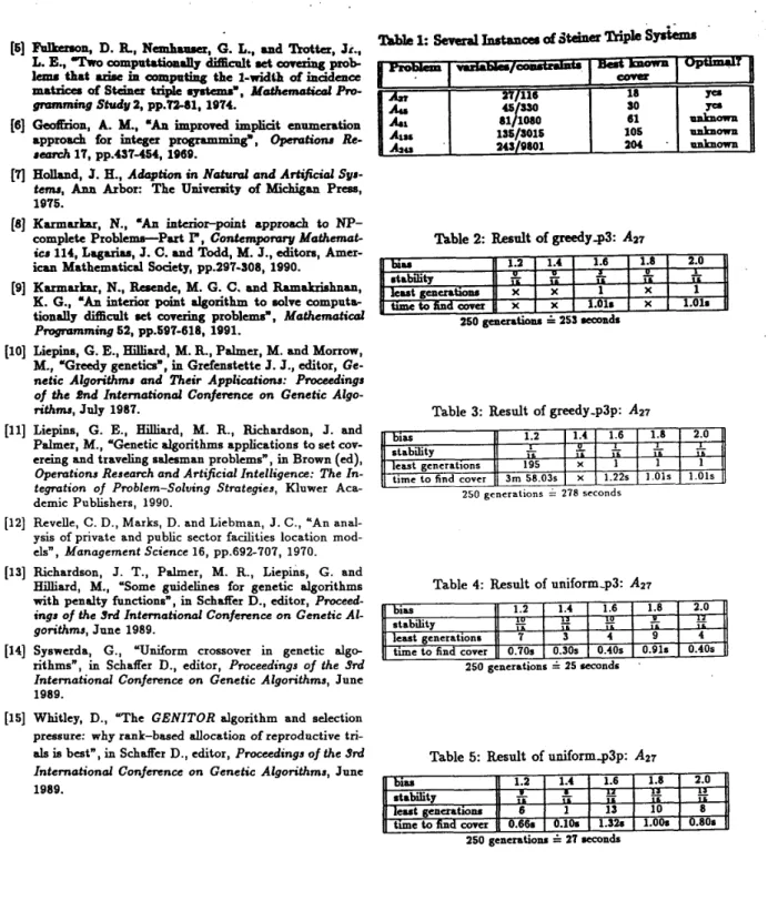
Table 2 t o Table 5 summarize the computational results of the above four genetic formulations on problem A27 whose optimal cover size is 18. The first row of these tables (i.e., bias) is the bias value in equation (2) and takes the values 1.2, 1.4, 1.6,

1.8 and 2.0. The second row (i.e., stability) is the proportion of optima found; i.e., stability means that the program meets optima m times in n runs. The third row (i.e., least generations) dedicates the smallest number of generations when the best so- lution is found. The fourth row shows the least amount of time required to identify the best solu- tion. Below each table there is also shown how many generations the corresponding formulation runs and the average total time it takes. From these we can compare the relative efficiency of all formulations.

From Table 2 to Table 5 we find that uniform crossover is about 10 times faster than greedy crossover and can produce more stable results than the greedy crossover; thai is, uniform crossover can find optima more quickly and easily than greedy crossover. In fact the greedy crossover is a little better than the ill-performed ChvAtal's heuristic men- tioned in [4].

We add our proposed mutation into uniform-p3p, resulting in a more complex genetic algorithm- mut -uniform-p3p.

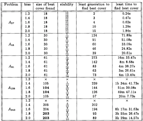
Table 6 summarizes the computational results of mut-uniform-p3p on problems A27 to A243. The

third column denotes the best cover size that mut-uniform-p3p finds corresponding to each bias value. Please notice that the fourth column (i.e., stability) is the proportion of cases when the optimal or best known covers described in Table 1

are found. The fifth column dedicates the smallest number of generations when the best cover is found. The sixth row shows the least amount of time in which the best solution is identified. Here

(4)

we set generation size to 400 for problem A81 and

250 for the others.

One important fact found in Table 6 is that mut-uniform-p3p finds a cover size 104 for A135.

This cover size is better than the currently best known solution 105. Here the stability includes the cases when cover size is 104 or 105. But it’s a pity that only one such case for 104 occurs in the 10 runs when bias is 1.6 or 1.8. Also note that in Table 6 mut-uniform-p3p finds a cover size 203 for A243.

This cover size is also better than the currently best known solution 204. The stability includes the cases when cover size is 203 or 204. But it’s a pity that only one such case for 203 occurs in the 10 runs when bias is 1.8 or 2.0. Our best solutions for A135

and A243 are shown in the Appendix.

5 Discussions

P3‘ does occasionally have difficulty finding solutions on smaller bias values. We have found several ignored rows (i.e., denoted by X ) in Table 6, indi- cating that using penalty function P3’ may produce a fittest (least-cost) solution which is not feasible at all. However we find that this occurrs only on smaller bias values and P3’ consistently finds lower cost solutions than P 3 . This fact suggests that more accurate estimates of the completion cost make better penalties.

In Table 6 we also find that when solving problem

A 2 7 , mut-uniform-p3p produces more stable results

than uniform-p3p in Table 5. That is, our proposed mutation operation can increase the stability of uniform-p3p. It is the same for larger problems.

From Table 6 we discover that

mut-uniform-p3p found cover sizes which are smaller t h a n t h e c u r r e n t l y b e s t known sizes for b o t h p r o b l e m s A135 a n d A243. Compared

with the results of Karmarkar’s interior-point ap- proach, our genetic algorithm is not as seriously af- fected by the local optima. The quality of solution found is highly related t o the bias value. For ex- ample, when solving problem A243, it takes over 8

hours to find cover size 204 on bias 1.6 while less than 4 hours t o find cover size 203 on bias 1.8 and 2.0.

6 Conclusions

In this paper, we have introduced a genetic algorithm approach for set covering problems. We have

In addition we demonstrate that uniform crossover is more efficient than the greedy crossover. We also propose a mutation operator that accelerates the convergence to the optimal solutions.

To illustrate the effectiveness of our resulting algorithm, mut-uniform-p3p, we apply it t o solve several instances of computationally difficult set covering problems. We have found optimal covers for two instances, A27 and A45, with known optimal solu-

tions and the best known covers for instances vary- ing in size from 81 variables and 1080 constraints t o 243 variables and 9801 constraints, i.e., A135

and A243, while taking much less time than the Kar-

markar approach experimented on the same set of test problems. In addition our genetic algorithm can find better solutions than the currently best known solutions for the two larger problems. Ear-

lier best approaches, including mathematical and stochastic algorithms, for these two problems were always trapped into a worse local optimum. This means that the ability of exploration and exploita- t i o n of genetic algorithms is much better than those of traditional optimization algorithms.

Appendix:

Best Solution of A135:

zj = 0, if j E { 3, 13, 14, 17, 23, 28, 34, 36, 48, 52, 53, 62, 66, 68, 70, 75, 76, 78, 80, 81, 94, 97, 101, 104, 105, 106, 118, 120, 121, 125, 134 }, optimal cover sizez104.

Our

Best Solutions

for A135

and

A243

Best Solution of A243:

zj = 0, i f j E { 5, 7, 9, 12, 13, 39,41, 48, 52, 59, 60, 63, 75, 79, 81, 89, 93, 99, 101, 102, 111, 119, 126, 129, 136, 143, 155, 194, 196, 200, 203, 209, 221, 223, 225, 227, 234, 235, 239, 240 }, optimal cover size=203.

References

[l] Arabeyre, J. P., Fearnley, J., Steiger, F. C. and Teather,

W., “The airline crew scheduling problem: a survey”,

Transportation Science 3, pp.140-168, 1969.

[2] Aubin, J., “Scheduling Ambulances”, Interfaces 22, pp.1-10, 1992.

[3] Chvbtd, V., “A greedy heuristic for the set cover- ing problem”, Mathematics of Operations Research 4,

pp.233-235, 1979.

[4] Feo, T. A. and Resende, M. G. C., “A probabilis- tic heuristic for a comDutationally difficult set cover-

described in detail the Procedure for generating a _{ing problem”, Operations Research Letters 8, pp.67-71,}

1989.

(5)

[SI Z ” n , D. RI Nunhauser, G. L., md %ta, Jr., L. E., ‘Two computrtioluny daficplt set cc+ng.prab- Laru that arise in computing the I-width of m a d a c e matrices d skinu triple sy”L=, Afothmrcrkcal - p r o -

gramming Studv 2, pp.72-8lIl974.

[SI GdEion, A. M., “An improved implicit enumeration approach for integer prog

-

2,

openations Re-

r e a d 17, pp.43744, 1969.

[7] Holland, J. H., Adaption i n Natud and Artificial Sys-

t e m , Ann Arbor: The University of Michigan Press,

1975.

[SI Karmarhu, N., “An intuior-poirtt approach to NP-

complete Problems--Part P’

,

Contemporary Mathemat- icr 114, Lagarins, J. C. and Todd, M. J., editom, Amer- ican Mathematied Society, pp.297-308, 1990.

[Q] Karmarhu, N., Reoende, M. G. C. and Ramakrishnan,

K. G., “An interior point algorithm to solve computa- tionally diScult set covering problemsa, M a t h e m a t i d Pmgmmming 52, pp.697-618, 1991.

(101 Liepins, G. E., Hilliard, M. R., Palmer, M. and Monow, M., “Greedy genetics”, in Grdenstettc J. J., editor, Ge- netic Algorithm and Their Applications: P d i n g s of the Snd Internationd Conference on Genetic Algo- rithms, July 1987.

[ll] Liepins, G. E., Hilliard, M. R., Richardson, J. and Palmer, M., “Genetic algorithms applications to set cov- ercing and traveling salesman problems”, in Brown (ed), Operations Research and Artificial Intelligence: The In- tegration of Problem-Solving Stmtegies, Kluwer Aca- demic Publishers, 1990.

[12] Revelle, C. D., Marks, D. and Liebman, J. C., “An anal- ysis of private and public sector facilities location mod-

els”, Management Science 16, pp.692-707, 1970. [13] Richardson, J. T., Palmer, M. R., Liepins, G. and

Hilliard, M., “Some guidelines for genetic algorithms with penalty functions”, in SchaiTer D., editor, Proceed- ings of the 3rd Intemational Conference on Genetic Al- gorithms, June 1989.

[14] Syswerda, G., “Uniform crossover in genetic a l g e rithms”, in Schaffer D., editor, Proceedings of the 3rd International Conference on Genetic Algorithms, June 1989.

[15] Whitley, D., “The GENITOR algorithm and selection pressure: why rank-based allocation of reproductive tri- als is best”, in SchaRer D., editor, Proceedings of the 3rd International Conference on Genetic Algorithms, June 1989.

Table 3: Result of greedy-p3p: A27

(6)

Table 6: Summary of results of mut-uniform-p3p

- least generation to

find best cover

least time to find best cover

2 0.24s 3 0.47s 4 0.62s 10 1.29s 15 1.84s 124 71.89s 91 51.08s 60 33.09s 46 24.82s 39 20.61s 273 16m 33.47s 142 8m 8.68s 83 4m 38.27s 63 3m 26.61s 73 4m 13.40s 239 l h 34m 41.73s 144 51m 39.08s 126 49m 47.11s 57 20m 7.73s 202 194 8h 17m 31.63s 93 3h 55m 26.47s 89 3h 29m 14.57s X X X X

Problem bias size of best stability cover found Ais6 A z r s -

G

1.4 105 104 1.6 1.8 104 2.0 105 10 1.2 X X 1.4 205 1.6 204 1.8 203 - 2.0 203 10 - Y - - 0 -

so

Y

- '40 -