三種不同資料結構下累積發生函數的無母數估計量研究

三種不同資料結構下累積發生函數的無母數估計量研究

Nonparametric Estimation of the Cumulative Incidence Function

under Three Types of Data Structures

研 究 生：陳建豪 Student：Chien-Hao Chen

指導教授：王維菁 Advisor：Weijing Wang

國 立 交 通 大 學

統 計 學 研 究 所

博 士 論 文

Submitted to Institute of Statistics College of Science

National Chiao Tung University in partial Fulfillment of the Requirements

for the Degree of PHD

in

Statistics

July 2008

Hsinchu, Taiwan, Republic of China

三種不同資料結構下累積發生函數的無母數估計量研究

學生：陳建豪

指導教授

王維菁

國立交通大學統計學研究所博士班

摘

要

在本論文中，我們考慮兩個在生物醫學上常被應用的量：累積發生函數以及長期

發生率；針對感興趣的發生原因，我們探討這兩個量的無母數估計。在三種不同

的資料結構下(競爭風險和治癒模式在右設限存在下、競爭風險在左截切存在

下)，我們分別應用三種不同的想法去得到無母數估計量：分解法，加權法以及

補值法。在本文中，我們證明出在每一種資料結構下，使用不用想法所得到的無

母數估計量都是相同的。另外，我們也利用數值分析來比較在競爭風險和治癒模

式下，何者的無母數估計量更為有效率。

Nonparametric Estimation of the Cumulative Incidence Function

under Three Types of Data Structures

student：Chien-Hao Chen

Advisors：Dr.

Weijin Wang

Institute of Statistics

National Chiao Tung University

ABSTRACT

In this thesis we consider nonparametric inference of the cumulative incidence

function for a particular type of failure and its long-term incidence rate, both of which

are useful descriptive measures for biomedical data with multiple endpoints. A unified

framework is provided to study different inference techniques under various

incomplete data structures. Specifically three approaches, namely decomposition,

weighting and imputation, are studied under data settings which include the

conventional competing risks data, the framework of a cure model and truncated

data. Identity between these methods for each data structure is examined. Numerical

examples are provided for comparing the first two data formulations.

Key words: Competing Risks; Cure models; Imputation; Inverse probability weighting;

Multi-state model; Nonparametric inference; Sufficient follow-up; Truncation.

誌

謝

首先，感謝我的指導教授王維菁老師的指導，使我在統計的領域中有更為寬廣

的視野，同時並不斷的指正、鼓勵，當我遇到困難時，指引我正確的研究方向，

才能順利的完成這篇論文。另外，也要感謝黃信誠老師，陳鄰安老師，徐南蓉老

師以及洪慧念老師撥冗前來擔任口試委員，並對本篇論文提出許多寶貴的意見，

讓我獲益非淺。

這幾年博士班的生活，衷心感謝統計所所有老師的諄諄教誨，以及用心的指

導。在此也感謝熱心的學長姐們，總是適時的給予幫助，使我解決了不少學習上

的難題。

最後，感謝家人以及好友們給予我的協助與鼓勵，有你們作後盾，我才能走的

那麼遠，並充滿勇氣的面對每一個挑戰。

陳建豪 謹誌于

國立交通大學

統計學研究所

Table of Contents

Chapter 1 Introduction

Chapter 2 Literature Review

Chapter 3 Competing Risks Data

3.1 Estimation of Cumulative Incidence Function 9 3.2 Estimation of Long-Term Incidence Rate 15

Chapter 4 Cure Model Framework

4.1 Estimation of Cumulative Incidence Function 22 4.2 Comparison of the two estimators 24 4.3 Estimation of long-term incidence rate 29

Chapter 5 Truncation Data

Chapter 6 Numerical Analysis

6.1 Simulation results 34

6.2 Analysis of Stanford Heart Transplant data 35

Chapter 7 Discussion

Chapter 1.

Introduction

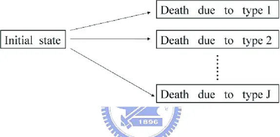
Multiple events data are commonly seen in many biomedical applications. Figure 1 depicts a common competing risks framework, in which there are J + 1 states, with state 0 being alive and states 1, 2, . . . , J corresponding to the J distinct types of death. Figure 2 describes another situation in which a subject receiving heart transplantation may experience two different paths (i.e. with/without rejection).

Figure 1: Competing risks of J distinct causes of death

Suppose that a person may experience one of J distinct types of failure or J different paths. Let T be the failure time of the first event and B be the indicator for the corresponding failure type taking values j = 1, . . . , J. The cumulative incidence function (CIF) for the jth cause of failure is defined as Fj(t) = Pr(T ≤ t, B = j). In the example

of heart transplant, let (B = 1) be the occurrence of rejection and (B = 2) be the death without rejection. In this case, F1(t) is the cumulative probability of experiencing

rejection by time t and F2(t) is the cumulative probability of death without rejection by

time t.

Under the conventional framework of competing risks, the cumulative incidence func-tion(CIF) can be considered as an extension of the Kaplan-Meier estimation with J = 1. Properties of the Kaplan-Meier estimator has been thoroughly studied in the literature. Specifically it is a product-limit estimator, satisfies the properties of redistribution-to-the-right and self-consistency, and is the nonparametric MLE. Recently Satten and Datta (2001) showed that the Kaplan-Meier estimator can also be expressed as an inverse-probability-of-censoring weighted average. In this thesis, we discuss how to generalize these inferential techniques to the estimation of CIF.

Most literature on CIF is developed under the competing risks framework. That is, one observes {(Ti, Bi)(i = 1, 2, . . . , n)} or its censored version. Nonparametric estimation

of Fj(t) in presence of right censoring has received substantial attention in the literature

(Anderson et al., 1993; Kalbfleisch and Prentice, 2002). The martingale expression of the nonparametric MLE(NPMLE) was given in Lin (1997), which is useful for large-sample analysis. Satten and Datta (1999) showed that the NPMLE can also be re-expressed by a product-limit representation with fractional risk sets. For the simple case of J = 2, two recent articles by Betensky and Schoenfeld (2001) and Wang (2003) studied the estimation of Fj(t) in the context of a two-state model. In practical applications, it

has been founded that the CIF estimate is often misused by practitioners. Golley et al. (1999) and Farley et al. (2001) explained the distinction between the estimate of the cumulative incidence function and the complement of the Kaplan-Meier estimator. We will also address this issue under the framework of cure model.

In this thesis, we apply different inference techniques to estimate Fj(t) and other

related quantities(i.e. the long-term incidence rate) under different types of data struc-tures. Chapter 2 reviews some relative papers about the cumulative incidence function. Chapter 3 considers the classical setting of competing risks data. Chapter 4 studies a different data formulation in the context of cure models in which subjects with B 6= j are treated as being cured and hence will never experience the cause of interest, B = j, despite of long-term follow-up. In Chapter 5, we extend the results to competing risks data subject to left truncation. Relationships between different inference approaches

are examined for each data structure. In Chapter 6 we provide numerical analysis to illustrate the difference between competing risks data and the data formulated based on the a cure model. Concluding remarks are given in Chapter 7.

Chapter 2.

Literature Review

In this Chapter, we focus on the competing risks setting. Let T be the failure time of the first event and B be the indicator for the corresponding failure type taking values

j = 1, . . . , J. Let S(t) = P r(T > t), F (t) = 1 − S(t) and

λ(t) = lim

∆t→0

Pr(T ∈ [t, t + ∆t)|T ≥ t)

∆t . (1)

The cumulative incidence function (CIF) of the jth event define as Fj(t) = Pr(T ≤

t, B = j) which is the cumulative probability of observing the jth event by time t.

However in practice, patients may drop out from the study or, at the end of the study, some may still have not developed any type of failure. Let C be the external censoring variable and assume that T and C are independent. Define Λj(t) =

R_t

0 λj(u)du, where

λj(t) is the cause-specific hazard function defined as

λj(t) = lim

∆t→0

Pr(T ∈ [t, t + ∆t), B = j|T ≥ t)

∆t . (2)

In presence of right censoring, observable variables become X = T ∧ C and ˜B = I(T ≤ C) · B. Let {(Ti, Ci, Bi) (i = 1, . . . , n)} be iid replications of (T, C, B). Observed data

can be expressed as {(Xi, δi, ˜Bi) (i = 1, . . . , n)}, where Xi = Ti∧ Ci and eBi = δi· Bi =

I(Ti ≤ Ci) · Bi.

Consider the special case of estimating S(t). The likelihood can be expressed as

n

Y

i=1

=

n

Y

i=1

[dΛ(Xi)]δiS(Xi).

It has been shown that the NPMLE places mass only at observed failure times. For the general case J > 1, the likelihood becomes

n Y i=1 {[ J Y j=1 dΛj(Xi)I( ˜Bi=j)] Y u≤Xi {1 − J X j=1 dΛj(u)}}.

Maximization of the above multinomial likelihood function, gives the MLE

dˆΛj(t) = P_n i=1_PI(Xi = t, eBi = j) n i=1I(Xi ≥ t) .

Lin(1997) showed that CIF has the following nice decomposition:

Pr(T ≤ t, B = j) = Z _t 0 Pr(T = u, B = j|T ≥ u)Pr(T ≥ u) = Z _t 0 S(u−)dΛj(u),

where S(u) = Pr(T > u) and Λj(t) =

R_t

0 λj(u)du. By a simple plug-in approach, Fj(t)

can be estimated by ˆ Fj(t) = Z _t 0 ˆ S(u−)dˆΛj(u), (3)

where ˆS(t) is the Kaplan-Meier estimator of Pr(T > t),

ˆ S(t) =Y u≤t {1 − P_n i=1_PI(Xi = u, δi = 1) n i=1I(Xi ≥ u) }

and dˆΛj(t) is the Nelson-Aalen estimator of dΛj(t), dˆΛj(t) = P_n i=1_PI(Xi = t, eBi = j) n i=1I(Xi ≥ t) .

Lin (1997) mentioned that (3) is also the NPMLE. The paper also derives the martingale expression of√n{ ˆF1(t) − F1(t)} in which weak convergence properties of the process can

be established. The results are useful for constructing confidence bands of Fj(t) based

on re-sampling techniques.

In survival analysis, there is a well-known relationship between the survival function and the cumulative hazard function. Specifically we have

S(t) = exp(−

Z _t

0

λ(u)du).

Therefore it seems natural to extend such a relationship to CIF and the cause-specific hazard function. However many researchers, including Golley et al. (1999) and Lin (1997) and Farley et al. (2001), found that

1 − Fj(t) ≥ exp(−

Z _t

0

λj(u)du).

We will clarify this issue by introducing another data structure, namely the cure model framework.

Chapter 3.

Competing Risks Data

Without external censoring, one observes {(Ti, Bi)(i = 1, . . . , n)}. The empirical

esti-mator of Fj(t) = E[I(T ≤ t, B = j)] is given by

¯ Fj(t) = n X i=1 I(Ti ≤ t, Bi = j)/n = n X i=1 Z _t 0 dI(Ti ≤ u, Bi = j)/n. (4)

Competing risks data in presence of right censoring, can be expressed as {(Xi, δi, ˜Bi)

(i = 1, . . . , n)}, where Xi = Ti∧ Ci and eBi = δi· Bi. Notice the indicator of interest,

I(Ti ≤ t, Bi = j) may be missing due to censoring and hence the empirical estimator

(4) is not applicable.

3.1.

Estimation of Cumulative Incidence Function

As mentioned in Chapter 2, the NPMLE of Fj(t) can be obtained explicitly by

ˆ FD j (t) = Z _t 0 ˆ S(u−)dˆΛj(u). (5)

Here we apply two useful principles for handling missing data to estimate Fj(t). One

way is treating I(X ≤ t, ˜B = j) as a biased proxy of I(T ≤ t, B = j) and then applying

the technique of weighting to correct the sampling bias. Notice that

E[I(X ≤ t, eB = j)

G(T −) |T ] = I(T ≤ t, B = j),

the following weighted average: ˆ F_jW(t) = 1 n n X i=1 I(Xi ≤ t, ˜Bi = j) ˆ G(Xi−) = 1 n Z u≤t P_n i=1dI(Xi ≤ u, ˜Bi = j) ˆ G(u−) , (6) where ˆ G(t−) = Y u<t {1 − P_n i=1_PI(Xi = u, eBi = 0) n i=1I(Xi ≥ u) }.

Imputation is another way to deal with incomplete observations. By writing Fj(t) =

R_t

0 Fj(du), it follows that

Fj(du) = E[I(T ∈ [u, u + du), B = j)] = E

h

E[I(T ∈ [u, u + du), B = j|X, eB)]

i

where E[I(Ti ∈ [u, u + du), Bi = j|Xi, eBi)] can be written as

I(Xi ∈ [u, u + du), eBi = j) + I(Xi < u, eBi = 0)

Pr(Ti ∈ [u, u + du), Bi = j)

S(Xi)

.

This approach yields the following self-consistent equation, bFI j(t) = R_t 0FbjI(∆u), where b FI j(∆u) = n X i=1 I(Xi = u, eBi = j)/n + n X i=1 I(Xi < u, eBi = 0) bFjI(∆u)/n bS(Xi). (7)

Note that the first component of bFI

j(∆u) is the original assigned mass at the failure time

point u and the second component is the mass re-distributed from previously censored observations. The estimator bFI

j(t) has the following explicit representation,

ˆ FI j(t) = Z u≤t P_n i=1dI(Xi ≤ u, ˜Bi = j) n −Pn_i=1I(Xi < u, ˜Bi = 0)/ ˆS(Xi) .

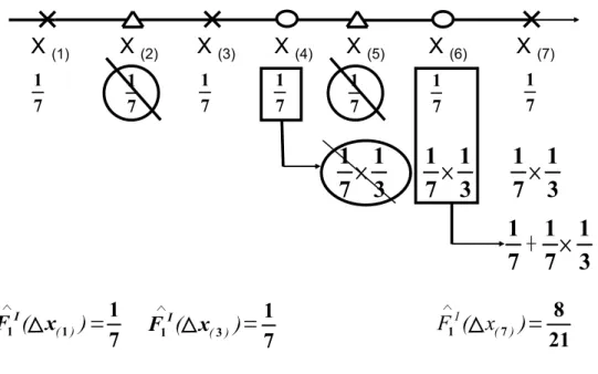
Figure 3 provides a simple example to illustrate the steps of mass re-distribution for estimating F1(t) when there are two types of failure. Let x(1) < x(2) < ... < x(n) be

ordered observations of Xi (i = 1, . . . , n) and δ(k) and eB(k) be the indicators associated

with x(k). At an observed point on the time line, the associated failure type is marked

as °, ×, and 4 for ˜B = 0, 1, 2, respectively. In the first step, every point is assigned

with mass 1/n = 1/7. As can be seen in (7), the mass assigned to points with ˜B = 2 has

no contribution to the calculation of bFI

1(t). Hence bF1I(x(1)) = 1/7 and bF1I(x(3)) = 2/7

since there are no censored observations with ˜B = 0 before these two points. The mass

assigned to the censored observation, x(4), will be evenly distributed to x(j) (j = 5, 6, 7)

and then the mass assigned to the censored observation, x(6), will be distributed to the

point on its right, x(7). The redistribution-to-the right algorithm works in the same way

as in the special case of Pr(B = 1) except that bFI

j(∆u) does not receive mass from other

1 7 1 7 1 7

X

X

X

X

X

X

X

Ø

1

1

7

3

Ø

1

1

7

3

Ø

1

1

7

3

,

Ø

1

1

1

7

7

3

F

x

(

)

1

7

(

)

F

x

1

7

F ( x

)

8

21

>

>

>

Figure 3: Mass calculation for estimation of ˆFI

1(t) based on the first data structure,

where ° : ˜B = 0;× : ˜B = 1;4 : ˜B = 2.

Now, we show that the above three estimators of Fj(t) are equivalent. Specifically

the jump sizes of the above estimators at time u are given by

ˆ

F_jD(∆u) = P_n

i=1I(Xi = u, eBi = j)

P_n

i=1I(Xi ≥ u)/ ˆS(u−)

, ˆ F_jW(∆u) = P_n i=1I(Xi = u, ˜Bi = j) n ˆG(u−) , and ˆ FI j(∆u) = P_n i=1I(Xi = u, ˜Bi = j) n −Pn_i=1I(Xi < u, ˜Bi = 0)/ ˆS(Xi) ,

where u = x(k) is an observed failure point with eB(k) = j.

Theorem 1:Identical relationship of bFD

j (∆u), bFjW(∆u) and bFjI(∆u)

According to the result of Satten and Datta (2001), we have ˆ S(u) = 1 − 1 n n X i=1 I(Xi ≤ u, δi = 1) ˆ G(Xi−) , (8) ˆ G(u−) = 1 − 1 n n X i=1 I(Xi < u, ˜Bi = 0) ˆ S(Xi) . (9)

By applying equation (9), it can be shown that the denominators of bFW

j (∆u) and bFjI(∆u)

are identical. In general, we can write

ˆ S(u−) ˆG(u−) = Y s<u ½ 1 − P_n i=1_PI(Xi = s, δi = 1) n i=1I(Xi ≥ s) − P_n i=1_PI(Xi = s, δi = 0) n i=1I(Xi ≥ s) + R(s) ¾ , where R(s) = ( P_n i=1I(Xi = s, δi = 1)) ( P_n i=1I(Xi = s, δi = 0)) (Pn_i=1I(Xi ≥ s))2 .

If there are no ties between failure and censored observations, R(s) should equal zero for all s and

ˆ S(u−) ˆG(u−) =Y s<u ½ 1 − P_n i=1I(Xi = s) P_n i=1I(Xi ≥ s) ¾ = 1 n n X i=1 I(Xi ≥ u) and hence bFW

j (∆u) = bFjD(∆u). Note that if there are ties between failures and

cen-sored observations, we can still make the same conclusion if we impose the conventional assumption that the failures had occurred just before the censored observations.

From now on, we write ˆFj(t) to denote any of the three representations. The

1 − F1(t) reduces to S(t) and 1 − ˆF1(t) reduces to the Kaplan-Meier estimator, ˆS(t).

Note that Satten and Datta (2001) has shown that

ˆ S(t) =Y u≤t {1 − P_n i=1_PI(Xi = u, δi = 1) n i=1I(Xi ≥ u) } = 1 − 1 n n X i=1 I(Xi ≤ t, δi = 1) ˆ G(Xi−) ,

which is a special case of equation (6). The numerator in ˆFj(∆u),

P_n

i=1I(Xi = u, ˜Bi = j), counts the number of observing

type j failure at time u. The denominator has three equivalent representations which measure the “effective sample size“ at time u adjusted for the underlying censoring mechanism. From the expression of ˆFW

j (∆u), we see that the effective sample size equals

n ˆG(u−) which is the (estimated) expected number of subjects that are not right censored

at time u. The expression of ˆFI

j(∆u) indicates that previously censored observations

should be excluded in the calculation of the effective sample size but their influence should be weighted according to their survival probabilities. The expression of ˆFD

j (∆u)

indicates that the effective sample size is larger than the number at risk since subjects who had died previously should be included in the adjusted sample size which accounts for the possibility of external censoring.

Despite of the equivalence, different representations of the some quantity may provide different applications. The connection with the nonparametric MLE is useful to establish the optimal property. The idea of imputation is related to the re-distribution to the right and self-consistent properties which may be adopted in other inference problems that

involve the covariate information or other censoring patterns. The weighted expression of ˆFW

j (t) is very useful for analytical analysis and may be generalized to other censoring

mechanisms if the effect of censoring can be formulated explicitly.

3.2.

Estimation of Long-Term Incidence Rate

The long-term incidence rate is defined as

πj = Pr(B = j) = lim

t→∞Pr(T ≤ t, B = j). (10)

Estimation of πj is not just a trivial extension of the previous results since as indicated

in (10), πj involves the tail information which may be missing if the quality of data

is the distribution of Fj(t) can not be recovered at the tail region. A crucial condition

which measures the quality of data for recovering the tail information is called “sufficient follow-up“. For competing risks data, define the following boundary points, τT = supt{t :

S(t) > 0},τC = supt{t : G(t) > 0}, and τX = supt{t : Pr(X > t) > 0}. Sufficient

follow-up requires τT ≤ τC, which means that the follow-up time is long-enough to recover the

whole information of S(t) despite of censoring. Let xj

max be the largest failure point for failure type j. When τT ≤ τC, τX = τT,

xj

max will be a valid estimator for τTj = supt{t : Pr(T > t, B = j) > 0} and hence

ˆ

πD

j = ˆFj(xjmax) will be a valid estimator for πj = Fj(τTj). Now, we show that ˆFj(xjmax)

the estimator, ˆ π_jW = n X i=1 I( ˜Bi = j) n ˆG(Xi−) .

Applying the idea of imputation, we need to estimate

E[I(Bi = j)| ˜Bi, Xi] = I( ˜Bi = j) + I( ˜Bi = 0)w(Xi), where w(Xi) = P r(Bi = j|Xi, ˜Bi = 0) = 1 S(Xi) Z _∞ Xi dFj(u).

This approach was considered by Wang (2003) under the framework of a two-path model, where πj represents the path probability. Using the plug-in principle, w(Xi) can be

estimated by ˆ w(Xi) = { Z _∞ Xi d ˆFj(u)}/ ˆS(Xi) (11)

and hence πj can be estimated by

ˆ πI j = 1 n n X i=1 {I( ˜Bi = j) + I( ˜Bi = 0) ˆw(Xi)}. Theorem 2: ˆπI j = ˆπWj = ˆπjD Proof: The estimator ˆπI j can be re-expressed as ˆ π_jI = 1 n n X i=1 n I( eBi = j) + I( eBi = 0) ˆw(Xi) o = 1 n n X i=1 ( I( eBi = j) + I( eBi = 0) ˆ S(Xi) " n X k=1 I(Xk > Xi, eBk = j) n ˆG(Xk−) #)

= 1 n n X i=1 I( eBi = j) + 1 n n X k=1 I( eBk= j) n ˆG(Xk−) " _n X i=1 I(Xk> Xi, eBi = 0) ˆ S(Xi) # . By equation (9), ˆ πI j = 1 n n X i=1 I( eBi = j) + n X k=1 I( eBk = j) n ˆG(Xk−) n 1 − ˆG(Xk−) o = n X k=1 I( eBk= j) n ˆG(Xk−) = ˆπW j .

Furthermore it follows that

ˆ πj = n X i=1 I( eBi = j) n ˆG(Xi−) = n X i=1 I(Xi ≤ xjmax, eBi = j) n ˆG(Xi−) = ˆFj(xjmax),

where xj_{max is the largest observed failure time for type j event.}

We see again that the three methods lead to the same estimator of πj, which will be

denoted by ˆπj.

For competing risks data, insufficient follow-up means that τT > τC. There will be

large censored observations at the tail so that ˆS(x(n)) > 0 and ˆG(x(n)) = 0, where x(n) is

the largest value of X. Consequently there will be some mass beyond xj

max which is not

estimable and hence ˆπj would underestimate πj. In fact, nonparametric estimation of

any quantity that involves the tail information has the problem of non-identifiability if follow-up is not sufficient. To accommodate the situation of insufficient follow-up, Wang (2003) suggested to impose an artificial assumption, Pr(B = j|T > τX) = πj, which

interest as in the whole support. The resulting estimator becomes ˘ π_jI = P_n i=1{I( ˜Bi = j) + I( ˜Bi = 0) ˆw(Xi)} ˘ n , (12) where ˘n = n − ncS(xˆ (n)) and nc = P_n

i=1I( ˜Bi = 0)/ ˆS(Xi). Alternatively, we can apply

the weighting approach to estimate πj by,

˘ πW j = 1 ˘ n n X i=1 I( eBi = j) ˆ G(Xi−) , and ˘ n = n − ncS(xˆ (n)) = n X i=1 I(δi = 1) ˆ G(Xi−) . Theorem 3: ˇπI

j(t) = ˇπWj (t)(adjusted for insufficient follow up)

Proof:

The original expression of ˘πI

j is given by ˘ π_jI = P_n i=1 n I( eBi = j) + I( e_S(XˆBi=0)_i) hP_n k=1 I(Xk>Xi, eBk=j) n ˆG(Xk−) io n − ncS(xˆ (n)) . To show n − ncS(xˆ (n)) = P_n i=1 I(δi=1) ˆ

G(Xi−), we need to consider the following two cases. Let

δ(n) be the indicator associated with x(n). If δ(n) = 1, which means that ˆS(x(n)) = 0, by

equation (8), we have Pn_i=1 I(δi=1)

ˆ

G(Xi−) = n. If δ(n) = 0 which implies that ˆG(x(n)) = 0 and

by equation (9), we have nc= P_n i=1 I( eBi=0) ˆ S(Xi) = n and hence n − ncS(xˆ (n)) = n(1 − ˆS(x(n))) = n X i=1 I(δi = 1) ˆ G(Xi−) .

Hence in either case, we have that n − ncS(xˆ (n)) = n X i=1 I(δi = 1) ˆ G(Xi−) ,

and it follows that

˘ πI j = P_n i=1I( eBi = j) . ˆ G(Xi−) P_n i=1I(δi = 1)/ ˆG(Xi−) .

Thus one can view ˘n as the sample size that only measures the identifiable region.

Chapter 4.

Cure Model Framework

In classical survival analysis, an implicit but sometimes implausible assumption is that every individual will eventually experience the event of interest. Cure models allow the possibility that a subject may not develop the event of interest despite of long-term follow-up. For more discussions on cure models, one can refer to the book by Maller and Zhou (1996). Data with multiple endpoints can be formulated in the context of cure models if a particular type of event, say type j, is of major interest. Under the framework of a cure model, those who will never experience this type of failure (B 6= j) are treated as being immune (cured, or non-susceptible) for the event of type j. One can define Tj as the hypothetical failure time such that

Tj = T · I(B = j) + ∞ · I(B 6= j).

For t < ∞ , the cumulative incidence function can be written as

Fj(t) = Pr(T ≤ t, B = j) = Pr(Tj ≤ t)

and hence its complement becomes

Sj(t) = Pr(Tj > t) = Pr(T > t, B = j) + Pr(B 6= j).

When there is more than one type of failure, 1 − πj = limt→∞Sj(t) > 0. In such a case,

It is useful to compare the failure time variables discussed in the paper via their hazard functions. The hazard functions for T and Tj are given by

λ(t) = lim ∆t→0 Pr(T ∈ [t, t + ∆t)|T ≥ t) ∆t (13) and ˜ λj(t) = lim ∆t→0 Pr(Tj ∈ [t, t + ∆t)|Tj ≥ t) ∆t , (14)

respectively. The relationship between a hazard function and its survival function holds for T and Tj such that

S(t) = Pr(T > t) = exp(− Z _t 0 λ(u)du), and Sj(t) = Pr(Tj > t) = exp{− Z _t 0 ˜ λj(u)du}.

In presence of competing risks, the cause-specific hazard for type j failure is defined as

λj(t) = lim

∆t→0

Pr(T ∈ [t, t + ∆t), B = j|T ≥ t)

∆t . (15)

Note that that λ(t) =PJ_j=1λj(t). It is easy to see that ˜λj(t) ≤ λj(t) since for t < ∞

Pr(Tj ∈ [t, t + ∆t)) = Pr(T ∈ [t, t + ∆t), B = j)

but Pr(Tj ≥ t) ≥ Pr(T ≥ t). The latter implies that the risk set at time t for Tj is a larger

Consequently Sj(t) = exp{− Z _t 0 ˜ λj(u)du} ≥ exp{− Z _t 0 λj(u)du}. (16)

In summary, we provide a new explanation of (16) which has been discussed in Lin (1997), and Gooley et al. (1997).

4.1.

Estimation of Cumulative Incidence Function

In the context of cure models, censored data based on Tj can be formulated as {( ˇXij, ˇδij) (i =

1, . . . , n)}, where ˇX_ij and ˇδ_ij are iid replications of ˇXj _{= T}

j ∧ C and ˇδj = I(Tj ≤ C)

respectively. It is important to note that ˇδ_ij = 0 corresponds to two possible situations of ˜Bi, namely ˜Bi = 0 and ˜Bi = k 6= j (k > 0), provided by the competing risks data

structure. However for the cure model considered here, when ˇδ_ij = 0, only ˇX_ij = Ci is

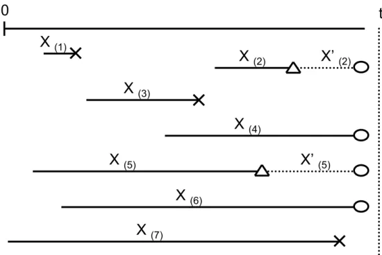
recorded and the information of other competing risks is ignored. Figure 4 illustrates the relationship between the two data structures. The first data structure can be converted to the second one if the failure time associated with ˜B = 2 is replaced by the time to

0

_t

X

X

X

X

X

X

X

X’

X’

Figure 4: Relationship between the two data structures. The difference is that the

second type of data extends the endpoint of the competing risk event marked by 4 to the

endpoint of external censoring marked by °.

By independence between Tj and C and equation (16), Sj(t) can be consistently

estimated by the Kaplan-Meier estimator,

ˇ Sj(t) = Y u≤t {1 − P_n i=1_PI( ˇXij = u, ˇδij = 1) n i=1I( ˇX j i ≥ u) }

and hence Fj(t) can be estimated by ˇFj(t) = 1 − ˇSj(t). As ˆFj(t), ˇFj(t) also has different

but equivalent representations. By similar arguments, one can show that

ˇ Fj(t) = n X i=1 I( ˇX_ij ≤ t, ˇδj_i = 1) n ˇG( ˇX_ij−) (17)

= Z u≤t P_n i=1dI( ˇX j i ≤ u, ˇδij = 1) n −Pn_i=1I( ˇX_ij < u, ˇδ_ij = 0)/ ˇSj( ˇXij) , (18)

which is also the nonparametric MLE, where

ˇ G(t) = Y u≤t {1 − P_n i=1I( ˇX j i = u, ˇδij = 0) P_n i=1I( ˇX j i ≥ u) }.

It should be mentioned that sometimes practitioners may estimate Fj(t) by the

comple-ment of the wrong Kaplan-Meier estimator

ˇ S0 j(t) = Y u≤t {1 − P_n i=1_PI(Xi = u, ˜Bi = j) n i=1I(Xi ≥ u) },

which actually estimates exp{−Λj(t)} but Sj(t) ≥ exp{−Λj(t)} as claimed in (16). The

misuse of 1 − ˇS0

j(t) to estimate Fj(t) has been noticed by many authors (Farley et al.,

2001; Gooley et al.,1999; Lin, 1997; Wang, 2003), just to name a few.

4.2.

Comparison of the Two Estimators

Now we compare the two estimators derived under different data structures based on their weighted expressions given in (6) and (17) respectively. We find that

I( ˇX_ij = u, ˇδ_ij = 1) = I(Xi = u, ˜Bi = j).

Hence these estimators only differ in the denominator that involves the estimator of

G(t). If the main purpose of inference was to estimate G(t), ˇG(t) is clear a better choice

since Pr(ˇδ = 0) ≥ Pr( ˜B = 0). In fact, ˇG(t) is less variable than ˆG(t). However the

turns out that a better estimator of G(t) does not necessarily yield a better estimator of

Fj(t). In the following, we show that ˆFj(t) has smaller asymptotic variance than ˇFj(t).

This phenomenon was first noticed by Tsai and Crowley (1998) in a different estimation problem that also involves inverse-probability-weighting. To better understand the effect of the estimator of G(t), we also evaluate two hypothetical estimators,

¯ Fj(t) = n X i=1 I(Xi ≤ t, ˜Bi = j) n ¯G(Xi−) (19)

where ¯G(t) =Pn_i=1I(Ci > t)/n, and

¯ F∗ j(t) = n X i=1 I(Xi ≤ t, ˜Bi = j) nG(Xi−) . (20)

Now, we show that although

0 = AVar(G(t)) ≤ AVar( ¯G(t)) ≤ AVar( ˇG(t)) ≤ AVar( ˆG(t)),

the relationship for the estimators of Fj(t) is reverse such that

AVar( ¯F_j∗(t)) ≥ AVar( ¯Fj(t)) ≥ AVar( ˇFj(t)) ≥ AVar( ˆFj(t)).

Theorem 4: AVar( ¯F∗

j(t)) ≥ AVar( ¯Fj(t)) ≥ AVar( ˇFj(t)) ≥ AVar( ˆFj(t)).

Proof:

Based on the martingale representation of ˆG(t), one can write √ n{G(t) − ˆG(t)} = n−1/2G(t) n X i=1 Z _t 0 dMci(u) Pr(X ≥ u) + op(1),

where

Mci(u) = I(Xi ≤ u, ˜Bi = 0) −

Z _u

0

I(Xi ≥ s)Λc(ds)

and Λc(s) is the cumulative hazard function of C. It follows that

√ n{ ˆFj(t) − Fj(t)} = 1 √ n n X i=1 Z _t 0 dI(Xi ≤ u, eBi = j) − dHj(u) G(u−) + √1 n n X i=1 Z _t 0 [ Z _u 0 dI(Xi ≤ s, eBi = 0) − I(Xi ≥ s)dΛc(s) Pr(Xi ≥ s) ]dFj(u) + op(1),

where Hj(t) = Pr(X ≤ t, eB = j). The asymptotic variance of ˆFj(t) equals Var(A(t)) +

2Cov(A(t), B(t)) + Var(B(t)), where

A(t) = Z _t 0 dI(X ≤ u, eB = j) − dHj(u) G(u−) , B(t) = Z _t 0 Z _u 0 dMc(s) Pr(X ≥ s)dFj(u) Mc(u) = I(X ≤ u, ˜B = 0) − Z _u 0 I(X ≥ s)Λc(ds). It follows that V ar(A(t)) = E[A2_{(t)] =} Z _t 0 dFj(u) G(u−) − F 2 j(t), V ar(B(t)) = Z _t 0 Z _t 0 E ·Z _u 0 dMc(s) Pr(X ≥ s)· Z _v 0 dMc(w) Pr(X ≥ w) ¸ dFj(u)dFj(v) = Z _t 0 Z _t 0 Z _u∧v 0 dhMc, Mci(s) Pr2_{(X ≥ s)} dFj(u)dFj(v),

= Z _t 0 Z _t 0 Z _u∧v 0 dΛc(s) Pr(X ≥ s)dFj(u)dFj(v). The covariance term equals

E[A(t)B(t)] = E (Z _t 0 dI(X ≤ v, eB = j) − dHj(v) G(v−) · Z _t 0 Z _u 0 dMc(s) Pr(X ≥ s)dFj(u) ) = Z _t 0 Z _t 0 1 G(v−) ·E ( h dI(X ≤ v, eB = j) − dHj(v) i · Z _u 0 dI(X ≤ s, eB = 0) − I(X ≥ s)dΛc(s) Pr(X ≥ s) ) dFj(u) = Z _t 0 Z _t 0 1 G(v−) ·E ( dI(X ≤ v, eB = j) · Z _u 0 dI(X ≤ s, eB = 0) − I(X ≥ s)dΛc(s) Pr(X ≥ s) ) dFj(u) = − Z _t 0 Z _t 0 1 G(v−)E ½ dI(X ≤ v, eB = j) · Z _u 0 I(X ≥ s)dΛc(s) Pr(X ≥ s) ¾ dFj(u) = − Z _t 0 Z _t 0 1 G(v−)E ½ dI(X ≤ v, eB = j) · Z _u 0 dΛc(s) Pr(X ≥ s) ¾ dFj(u) = − Z _t 0 Z _t 0 Z _u∧v 0 dΛc(s) Pr(X ≥ s)dFj(u)dFj(v).

Asymptotic variance of√n{ ˆFj(t) − Fj(t)} equals ·Z _t 0 dFj(u) G(u−) − F 2 j(t) ¸ − Z _t 0 Z _t 0 Z _u∧v 0 dΛc(s) Pr(X ≥ s)dFj(u)dFj(v). (21) Hence asymptotic variance of√n{ ˇFj(t) − Fj(t)} can be derived in the same way, which

is given by ·Z _t 0 dFj(u) G(u−) − F 2 j(t) ¸ − Z _t 0 Z _t 0 Z _u∧v 0 dΛc(s) Pr( ˇX ≥ s)dFj(u)dFj(v). (22)

Notice that (21) and (22) only differ by one term in the the second component. Because Pr( ˇX ≥ s) ≥ Pr(X ≥ s), it is easy to see that

AVar(√n{ ˇFj(t) − Fj(t)}) ≥ AVar(

√

n{ ˆFj(t) − Fj(t)}).

The asymptotic variance of √n{ ¯Fj(t) − Fj(t)} is

·Z _t 0 dFj(u) G(u−) − F 2 j(t) ¸ − Z _t 0 Z _t 0 Z _u∧v 0 dΛc(s) Pr(C ≥ s)dFj(u)dFj(v), (23) which can be further simplified as

·Z _t 0 dFj(u) G(u−) − F 2 j(t) ¸ − Z _t 0 Z _t 0 ( 1 G(u ∧ v)− 1)dFj(u)dFj(v),

and the asymptotic variance of√n{ ¯F∗

j(t) − Fj(t)} is Z _t 0 dFj(u) G(u−) − F 2 j(t). (24) It is clear that AVar( ¯F∗

4.3.

Estimation of long-term incidence rate

In presence of external censoring, the non-identifiable region for competing risks data refers to the set, {t : t > τT ∧ τC} and the non-identifiable region for data of the cure

model is {t : t > τ_Tj ∧ τC}. It is important to note that τTj < τT. Clearly the second set

is larger than the first one. When follow-up is sufficient, we have τ_Tj < τT < τC and both

data structures provide enough information for estimating π. However when follow-up is not sufficient, the two data structures contain different level of information about the tail distribution.

Based on the second type of data {( ˇX_ij, ˇδ_ij) (i = 1, . . . , n)}, sufficient follow-up re-quires τ_Tj ≤ τC, which implies that the length of follow-up is long enough to observe all

the susceptible with B = j. If τ_Tj ≤ τC, πj can be consistently estimated by the following

three expressions ˇ πj = 1 − ˇSj(xjmax) = n X i=1 I(ˇδ_ij = 1) n ˇG( ˇX_ij−) = 1 n n X i=1 © I(ˇδ_ij = 1) + I(ˇδ_ij = 0) ˇw( ˇX_ij)ª, where ˇ w(t) = P_n k=1I( ˇXkj > t, ˇδkj = 1) ˇFj(∆ ˇXkj) ˇ Sj(t) .

For the cure model, insufficient follow-up means that τ_Tj > τC. Consequently ˇπj

also underestimates πj. For competing risks data, the probability of the non-identifiable

region {t : t > τT ∧ τC} is identifiable and is estimated by ˆS(x(n)) which provides the

τX) = πj. However for the second data structure, the mass of the non-identifiable region

{t : t > τ_Tj ∧ τC} is still not identifiable without imposing distributional assumptions.

It seems that it is impossible to construct a valid estimator of πj nonparametrically.

The book by Maller and Zhou (1996) has thorough discussions on the problem of non-identifiability in the context of cure models.

Chapter 5.

Extension to Truncation Data

We discuss whether the two suggested estimation principles can be extended to incor-porate left truncation. Suppose that T is the age when the first failure occurs and B is the corresponding failure type. Let L be the age that a subject enters the study. If the sample only includes those who have not developed any type of failure, we can imagine that the sample is subject to left truncation such that only those with T > L can be included in the sample. Let (Ti, Bi, Li) (i = 1, . . . , m) be a random sample of

(T, B, L). Under left truncation, we only observe the sample (Ti, Bi, Li) (i = 1, . . . , n)

with Ti > Li and m is unknown. Let FL(t) = Pr(L ≤ t) be the distribution function of

L. For truncated data, the marginal functions S(t) and FL(t) can be estimated by the

Lynden-Bell estimators ˜ S(t) = Y u≤t {1 − P_n i=1I(Ti = u, Li ≤ u) P_n i=1I(Li ≤ u ≤ Ti) }, ˜ FL(t) = Y u>t {1 − P_n i=1I(Li = u, Ti ≥ u) P_n i=1I(Li ≤ u ≤ Ti) }.

We first study estimation of m and α = Pr(T ≥ L). Let F (t) = 1 − S(t). Based on the decomposition that α = R FL(u)dF (u), we have ˜αD =

R _˜

FL(u)d ˜F (u), where

˜

F (t) = 1 − ˜S(t). Based on another less straightforward decomposition,

we may estimate α by

˜

α(t) = P_n F˜L(t) ˜S(t−)

i=1I(Li ≤ t ≤ Ti)/n

.

The weighting approach can be applied based on the relationship

E[ 1 FL(T ) |T ≥ L] = 1 Pr(T ≥ L)E[ I(T ≥ L) FL(T ) ] = 1 α,

which implies that α can be estimated by

˜ αw = {1 n n X i=1 1 ˜ FL(Ti) }−1.

It is important to mention that, in presence of truncation, the method of imputation seems not applicable since an truncated observation is completely missing and even its existence is unknown. He and Yang (1998) considered estimation of α and, in their Theorem 2.2, it is shown that ˜α(t) = ˜αD _{for any t such that} Pn

i=1I(Li ≤ t ≤ Ti) > 0.

Now, we show that ˜α(t) = ˜αD _{= ˜α}w_.

Theorem 5: ˜α(t) = ˜αD _{= ˜α}w

Proof:

From (2.8)of He and Yang (1998), we have Pn_i=1I(Ti = t)/n = ˜FL(t)∆ ˜F (t)/˜αD and

hence ∆ ˜F (t) = ˜αDPn

i=1I(Ti = t)/n ˜FL(t). By taking summation over all t on both

sides of the previous identity, we have

1 = n X i=1 ∆ ˜F (Ti) = ˜αD n X i=1 1 n ˜FL(Ti) ,

which means that ˜αD _{= {}1

n

P_n

From the above two estimators, we see the jump sizes at time u are given by ˜ F_jw(∆u) = {1 n n X i=1 1 ˜ FL(Ti) }−1· { P_n i=1I(Ti = u, Bi = j, Ti ≥ Li) n ˜FL(u) }, and ˜ FD j (∆u) = { P_n i=1I(Ti = u, Bi = j, Ti ≥ Li) P_n

i=1I(Li ≤ u ≤ Ti)/ ˜S(u−)

}.

Proving ˜Fw

j (∆u) = ˜FjD(∆u) is the same as showing ˜αD = ˜αw.

It follows that the total sample size m can be estimated by

˜ m = R _˜ n FL(u)d ˜F (u) = n X i=1 1 ˜ FL(Ti) = P_n i=1I(Li ≤ t ≤ Ti) ˜ FL(t) ˜S(t−) . (26)

Since Pn_i=1I(Ti = u, Bi = j)/n is an estimator of Fj(∆u)Pr(L < u)/α, it follows that

Fj(∆u) can be estimated by

P_n

i=1I(Ti = u, Bi = j)/ ˜m ˆFL(u), where ˜m can be any of

the above estimators in (26). The method of decomposition yields the estimator

˜ Fj(t) = Z u≤t ˜ S(u−)d˜Λj(u), where ˜ Λj(u) = Z Pn i=1_PI(Ti = u, Bi = j, Li ≤ u) n i=1I(Li ≤ u ≤ Ti) .

Chapter 6.

Numerical Analysis

6.1.

Simulation Results

The purpose of the simulation studies was to examine the performance of ˆF1(t) and

ˇ

F1(t) in finite samples (i.e. n = 100 and n = 200). Suppose that there are two types of

failure. The indicator I(B = 1) was generated from a Bernoulli random variable with probability π1 and the latency variable for each type Tj|B = j was generated from an

exponential distribution such that Pr(Tj > t|B = j) = exp(−λj) (j = 1, 2). The failure

time of the first event was set to be T = I(B = 1)T1+ I(B = 2)T2. The independent

censoring variable C was generated from U(0, m). Hence

Pr( ˜B = 1) = Pr(ˇδ = 1) = π1· Pr(T ≤ C|B = 1),

which measures the probability of observing the first type of failure by time t in presence of external censoring. In addition to the two proposed estimators ˆF1(t) and ˇF1(t), the

hypothetical estimators ¯F1(t) and ¯F1∗(t) in (19) and (20) were also evaluated.

Table 1 displays the average bias and standard deviation of each estimator, based on 500 replications, when π1 = 0.9, λ1 = 0.8, λ2 = 1 and m = 5 which gives Pr( ˜B = 1) ≈

0.67. We see that the correct order of the asymptotic variances for the four estimators shown in (25) has already appeared when n = 100. The discrepancy gets larger when

t approaches to the tail. Table 2 shows the results when π1 = 0.9, λ1 = 0.8, λ2 = 1

estimators improves as n or Pr( ˜B = 1) increases. Table 3 displays the results when π1 = 0.5, λ1 = 0.8, λ2 = 1 and m = 10 which gives Pr( ˜B = 1) ≈ 0.44. Although

the relative performances of the four estimators are consistent with the previous two settings, the differences become less obvious when π1 and Pr( ˜B = 1) decrease.

6.2.

Analysis of Stanford Heart Transplant Data

For illustration, the methods discussed in the article were applied to analyze the Stanford transplant data (Crowly and Hu, 1977). The event of interest (B = 1) is rejection and the competing risk (B = 2) is death without rejection. Among 65 patients, 29 with rejection ( ˜B = 1), 12 died without rejection ( ˜B = 2) and 24 were censored ( ˜B = 0).

For the 12 patients without rejection ( ˜B = 2), we set ˇX = C, which is the time from

the date of acceptance to the end of the study in April 1974. The quantity of interest is F1(t) which represents the cumulative incidence probability of experience rejection by

time t. The two estimated cumulative incidence functions, ˆF1(t), and ˇF1(t), were shown

in Table 4 and plotted in Figure 5. When t > 500, we see that the discrepancy between ˆ

F1(t) and ˇF1(t) increases as t gets larger. It seems that ˇF1(t) is less reliable because of

heavy censoring in T1, the time to death without rejection.

To estimate π1, the probability of rejection, a naive estimate is 29/65 = 0.446.

If Pr( ˜B = 0) is very small, this estimate may be reliable. However in the present

reasonable. Applying our methods, the evidence of insufficient follow-up is clear since ˆ

S(x(n)) = ˆS(1350) ≈ 0.209. We found that x1max = 1350 and ˆπ1 = ˆF1(x1max) = 0.548.

The modified estimator in (12), which accounts for the unassigned mass in the tail, is ˘

π1 = 0.693. Which is a more reasonable estimator of π1 than the naive estimator.

time cu mu la ti v e i n ci den ce f un ct io n 0 500 1000 1500 2000 0 .0 0 .1 0 .2 0 .3 0 .4 0 .5

Figure 5: Two estimators of the cumulative incidence probability for the time to

rejection by time t based on the Stanford Heart Transplant data. ˆF1(t) : the dashed line;

ˇ

Chapter 7.

Discussion

We have demonstrated that, as the Kaplan-Meier estimator, the cumulative incidence function can be estimated via different approaches. We prove that these representations are equivalent under the settings discussed in the thesis. For future applications, these techniques may offer different alternatives in other contexts such as interval censoring or regression problems.

The inverse-probability-weighting representation is particularly useful in simplifying analytic work which has led to closed-form expressions of the asymptotic variances as shown in (21) and (22). It also allows us to compare the two estimators ˆFj(t) and

ˇ

Fj(t) analytically. The second structure allows one to use existing statistical packages

to estimate 1 − Fj(t) by the Kaplan-Meier estimator. However since the data ignores

the information provided by other competing risks, the resulting estimator has larger variance and also it seems unlikely to estimate the long-term incidence rate if the follow-up period is not long enough. In fact, the simulations indicate that the two estimators have larger difference in the tail region. In the extension to truncated data we found that the imputation fails but the weighting method still works.

Shen (2003) showed that the Lynden-Bell estimator for the left-truncation data can be expressed as inverse-probability-weighted average. To estimate the truncation prob-ability with left-truncated and right-censored data, Shen (2005) proposed two different

References

Andersen, P. K., Borgan, ∅., Gill, R. D., and Keiding, N. (1993). Statistical Models

Based on Counting Processes, New York: Springer-Verlag.

Betensky, R. A. and Schoenfeld, D. A. (2001). Nonparametric estimation in a cure model with random cure times. Biometrics, 57, 282-286.

Crowley, J. and Hu, M. (1977). Covariance analysis of heart transplant survival data,

Journal of the American Statistical Association, 72, 27-36.

Farley, T. M. M., Ali, M. M. and Slaymaker, E. (2001). Competing approaches to analysis of failure times with competing risks. Statistics in Medicine, 20, 3601-3610.

Fine, J. P. and Gray, R. J. (1999). A proportional hazards model for the subdistribution of a competing risk, Journal of the American Statistical Association, 94, 496-509.

Fine, J. P. (1999). Analyzing competing risks data with transformation models. J. R.

Statist. Soc. B, 61, 817-830.

Gooley, Leisenring, W., Crowley, J. and Storer, B. E. (1999). Estimation of failure probabilities in the presence of competing risks: mew representation of old esti-mators. Statistics in Medicine, 18, 695-706.

Kalbfleisch, J. D. and Prentice, R. L. (2002). The Statistical Analysis of Failure Time

Data, Wiley-Interscience.

Lin, D. Y. (1997). Non-parametric inference for cumulative incidence functions in competing risks studies. Statistics in Medicine, 16, 901-910.

Maller, R. A. and Zhou, S. (1996). Survival Analysis with Long-Term Survivors, Wiley: New York.

Satten, G. A. and Datta, S. (1999). Kaplan-Meier representation of competing risk estimates. Statistics and Probability Letters, 42, 299-304.

Satten, G. A. and Datta, S. (2001). The Kaplan-Meier Estimator as an Inverse-Probability-of-Censoring Weighted Average. The American Statistician, 55, 207-210.

Shen, P.-S. (2003). The product-limit estimates as an Inverse-Probability-Weighted Average. Communications in statistics, Part A-Theory and Methods, 32, 1119-1133.

Shen, P.-S. (2005). Estimation of the truncation probability with left-truncated and right-censored data. Nonparametric Statistics, 17, 957-969.

Tsai, W.-Y. and Crowley, J. (1998). A note on nonparametric estimators of the bivari-ate survival function under univaribivari-ate censoring. Biometrika, 85, 573-580.

Wang, W. (2003). Nonparametric estimation of the sojourn time distributions for a multi-path Model. J. R. Statist. Soc. B, 65, 921-936.

Table 1: Performance of ˆF1(t), ˇF1(t), ¯F1(t), and ¯F1∗(t) when π1 = 0.9 and Pr( ˜B = 1) ≈ 0.67. n=100 n=200 Fn(t) Fˆ1(t) Fˇ1(t) F¯1(t) F¯1∗(t) Fˆ1(t) Fˇ1(t) F¯1(t) F¯1∗(t) 0.1 0.339 0.340 0.340 0.342 0.272 0.272 0.273 0.275 (-0.982) (-0.982) (-0.983) (-1.051) (-0.522) (-0.522) (-0.522) (-0.587) 0.3 1.05 1.05 1.05 1.13 0.798 0.798 0.812 0.86 (-0.984) (-0.987) (-0.978) (-1.66) (-0.521) (-0.524) (-0.523) (-1.21) 0.5 1.73 1.74 1.82 1.98 1.28 1.29 1.35 1.57 (-1.06) (-1.07) (-1.06) (-3.27) (-0.530) (-0.538) (-0.535) (-2.8) 0.7 2.37 2.46 2.78 3.05 1.70 1.78 1.99 2.35 (-1.02) (-1.06) (-1.05) (-6.48) (-0.46) (-0.47) (-0.49) (-5.9) The first number in each cell is the standard deviation (×10−2_{), and the second number}

in parentheses is the average bias (×10−3_).

Table 2: Performance of ˆF1(t), ˇF1(t), ¯F1(t), and ¯F1∗(t) when π1 = 0.9 and Pr( ˜B = 1) ≈

0.79. n=100 n=200 Fn(t) Fˆ1(t) Fˇ1(t) F¯1(t) F¯1∗(t) Fˆ1(t) Fˇ1(t) F¯1(t) F¯1∗(t) 0.1 0.252 0.252 0.253 0.260 0.173 0.173 0.174 0.176 (-0.99) (-0.99) (-0.99) (-0.99) (-0.493) (-0.493) (-0.492) (-0.496) 0.3 0.758 0.759 0.768 0.831 0.529 0.529 0.530 0.570 (-0.992) (-0.99) (-0.99) (-0.97) (-0.50) (-0.501) (-0.496) (-0.517) 0.5 1.22 1.23 1.28 1.47 0.82 0.824 0.868 1.05 (-1.0) (-0.994) (-0.98) (-0.94) (-0.496) (-0.493) (-0.481) (-0.528) 0.7 1.62 1.67 1.86 2.30 1.14 1.17 1.33 1.66 (-0.994) (-0.975) (-0.931) (-0.86) (-0.492) (-0.475) (-0.431) (-0.513) 0.9 2.19 2.65 3.19 3.92 1.67 2.25 2.58 3.05 (-1.98) (-1.81) (-1.79) (-1.67) (-1.19) (-0.98) (-0.92) (-1.02) The first number in each cell is the standard deviation (×10−2_{), and the second number}

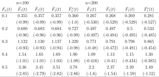
Table 3: Performance of ˆF1(t), ˇF1(t), ¯F1(t), and ¯F1∗(t) when π1 = 0.5 and Pr( ˜B = 1) ≈ 0.44. n=100 n=200 Fn(t) Fˆ1(t) Fˇ1(t) F¯1(t) F¯1∗(t) Fˆ1(t) Fˇ1(t) F¯1(t) F¯1∗(t) 0.1 0.355 0.357 0.357 0.360 0.267 0.268 0.269 0.281 (-0.99) (-0.99) (-0.99) (-1.0) (-0.530) (-0.529) (-0.529) (-0.527) 0.2 0.680 0.683 0.684 0.727 0.497 0.497 0.5 0.533 (-0.96) (-0.96) (-0.96) (-0.99) (-0.497) (-0.494) (-0.495) (-0.485) 0.3 1.122 1.130 1.137 1.220 0.771 0.791 0.798 0.865 (-0.93) (-0.93) (-0.94) (-0.98) (-0.48) (-0.472) (-0.481) (-0.454) 0.4 1.54 1.65 1.69 1.90 1.09 1.13 1.15 1.30 (-1.01) (-1.01) (-1.03) (-1.08) (-0.416) (-0.41) (-0.434) (-0.385) 0.5 3.36 3.45 3.51 3.78 2.2 2.37 2.39 2.49 (-2.85) (-2.79) (-2.82) (-2.86) (-1.6) (-1.54) (-1.59) (-1.52) The first number in each cell is the standard deviation (×10−2_{), and the second number}

in parentheses is the average bias (×10−3_).

Table 4: Comparison of ˆF1(t), ˇF1(t), based on Stanford heart transplant data.

t Fˆ1(t) Fˇ1(t) t Fˆ1(t) Fˇ1(t) 13 0.016 0.016 161 0.306 0.306 29 0.047 0.047 280 0.340 0.342 39 0.063 0.063 589 0.375 0.378 50 0.128 0.128 624 0.399 0.403 54 0.177 0.177 994 0.480 0.494 63 0.209 0.209 1106 0.511 0.528 66 0.258 0.257 1350 0.548 0.571 68 0.274 0.273 136 0.29 0.29