Pergamon
Int. J. Mach. Tools Manufact. Vol. 37, No. 4, pp. 409-423, 1997 O 1997 Elsevier Science Ltd Printed in Great Britain. All rights re.fred 0890-6955/97517.00 + .00
PII: S0890-6955(96)00063-6
A N A L Y S I S O F A N E Q U I V A L E N T D R A W B E A D M O D E L F O R T H E F I N I T E E L E M E N T S I M U L A T I O N O F A S T A M P I N G P R O C E S S
FUH-KUO CHENt~: and JIA-HONG LIUI" (Received 19 Feburary 1996)
Abstract--In order to facilitate the three-dimensional finite element analysis for the stamping process, an equivalent drawbead model was adopted to simulate the restraining effects produced by the real drawbead. In the present study, the restraining force exerted by the real drawbead was first computed by the finite element simulation, and the optimum pseudo drawing speed and mesh sizes for both the drawbead and sheet metal employed in the computation were determined through a systematic approach. The computed restraining force was then assigned to a regular mesh which replaced the mesh of the real drawbead. This constitutes the equivalent drawbead model, which avoids the extremely fine mesh required to describe the deformation of sheet blank in the drawbead area. In consequence, a huge amount of computation time can be saved. The accuracy of the finite element simulations using the equivalent drawbead model was validated by both the experimental data and the theoretical predictions. © 1997 Elsevier Science Ltd. All rights reserved
1. INTRODUCTION
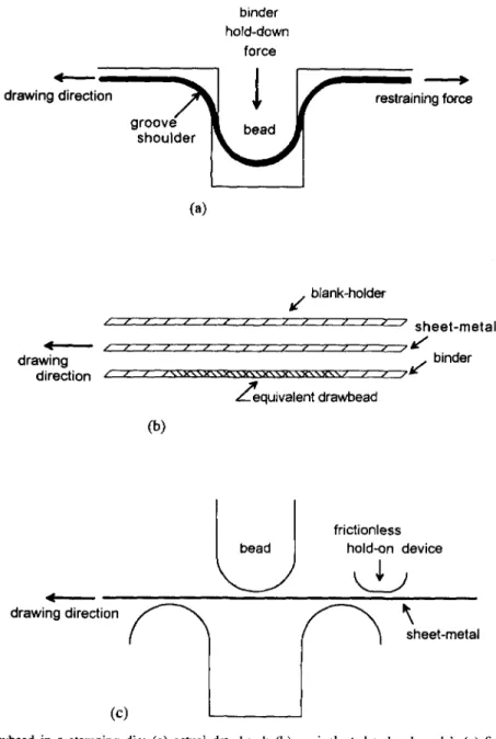
The stamping process is a long-established practice for mass production of sheet-metal parts. In the forming operation, the sheet metal is first clamped by the binders around the periphery of the die cavity, and is subsequently drawn into the die cavity by a moving punch to form the desired shape. During the draw, the binders exert a restraining force to control the amount of sheet metal moving into the die cavity by the friction generated between the binders and the sheet metal. For some forming operations, the restraining force provided by friction alone is not enough to control the metal flow, and drawbeads must be added to the binders for reinforcement. The drawbead is a small bead located on the binder surface and is matched by a groove on the die surface, as shown in Fig. l(a). The sheet-metal forming technology is then mainly focused on the design of die surfaces including the drawbeads, which depends mostly on the experience and know-how of engin- eers.
It was not until the 1980s that the finite element method was effectively used to analyze the sheet-metal forming process [1-3]. However, owing to the limitation of computational capability, most of the research was limited to the two-dimensional analyses at that time. Recently, owing to the advance of computer technology, the applications of three- dimensional finite element methods to this field have been developed [4-7]. Among them, the explicit time integration method [6] appears to be the most practical one for simulating the stamping processes because of its advantages of fast computation algorithms over the implicit integration method. One of the characteristics of the explicit finite element method is that the time step for integration is limited by a critical time increment AT=L/c, where L is the characteristic length of the minimum element in the mesh, and c is the wave speed traveling in the sheet metal, respectively. It is obvious that the computation time for the simulation of a stamping process using the explicit finite element method is partly governed by the size of the minimum element, which is therefore desired to be as large as possible for a mesh system to be analyzed.
Since the size of the drawbeads is usually very small compared with the remaining portion of the die surface, the sheet metal which is pulled through the drawbeads during drawing must be modeled by very small elements to reflect the effect of bending defor-
tDepartment of Mechanical Engineering, National Taiwan University, Taipei, Taiwan, R.O.C. SAuthor to whom correspondence should be addressed.
410 F u h - K u o Chen and Jia-Hong Liu
drawing direction
binder
hold-down
force
g r o o v ~ ~
shoulder
restraining force
(a) f f J I [ f f jdrawing
direction " -" /
blank-holder
J
z z z'.-
z z ,- ,- ,- ,- ,, " /sheet-metal
/ .," / " ' / , ( /" /" (" ¢" . / /" ,4 / ~ k /binder
~ q u i v a l e n t d r a w b e a d (b)be•
frictionless
hold-on device
drawing direction
/ ~
~heet-metal
(c)Fig. 1. D r a w b e a d in a stamping die: (a) actual drawbead; (b) equivalent drawbead model; (c) finite element model.
marion of the sheet metal around the drawbeads. A finite element model with such small elements results in an increase in the number of elements and contact segments and a decrease in the minimum time step and, in consequence, proves to be uneconomical in terms of the computation time. Hence, an equivalent drawbead model was developed [4] to replace the full-scale physical modeling of the drawbead in the finite element simulation of a sheet-metal forming operation to save computation time. In the equivalent drawbead model, the actual drawbead is replaced by its projection on to the binder surface, i.e. a flat surface which has the same width as the actual drawbead, and a regular mesh is constructed for the flat surface, as shown by the shaded area in Fig. l(b). The restraining force exerted by the actual drawbead is then to be calculated and assigned distributively to the nodes in the regular mesh of the equivalent drawbead following the virtual work principle. The main idea is that the sheet metal passing through the equivalent drawbead model will be subjected to the same restraining force as that exerted by the actual drawbead without using an extremely fine mesh. Therefore, an accurate estimation of the restraining force due to the actual drawbead is essential for setting up the equivalent drawbead model. In the present study, the restraining force calculated by the three-dimensional explicit
Analysis of an equivalent drawbead model 411 finite element method was investigated and the results were validated by the experimental data published in the literature [8, 9]. Also, the optimum mesh size employed in the simulation was examined through a systematic approach. A great saving in computation time achieved by using the equivalent drawbead model instead of the actual drawbead shape in the simulation was confirmed.
All the simulations performed in the present study were run on an HP735 workstation with the use of the finite element program PAM-STAMP.
2. DRAWBEAD RESTRAINING FORCE
The configurations of drawbeads used in the stamping operations vary a great deal, depending on the stamping requirements. For simplicity, a typical drawbead which consists of a semicylindrical bead fitting into a groove on the opposing binder surface, as sche- matically shown in Fig. l(a), is adopted to define the configuration of the model to be analyzed. When the punch draws the sheet metal into the die cavity after the binder closure, the sheet metal passing through the drawbead is subjected to a bending around the groove shoulder, an unbending at the half bead, and a repeated sequence at the bead exit and the groove shoulder. These bending and unbending deformations together with the frictional force account for the drawbead restraining force as well as the binder hold-on force. Quite a few theoretical and experimental research works on both the restraining force and hold- on force have been reported [8-13] since Nine [8] proposed the drawbead simulator in 1982. Among them, the experimental data and the theoretical predictions reported by Nine [8] and Wang et al. [9] were used to validate the the finite element results obtained in this study.
In the finite element simulations using the explicit time integration, the drawing speed is usually raised to a fictitious value of several orders higher than the actual speed to reduce the CPU time. A very large pseudo drawing speed is likely to affect the accuracy of the solution. Hence, in order to obtain an accurate restraining force using the explicit finite element method within an economical computation time, the optimum pseudo draw- ing speed and mesh size used in the simulations were determined on the basis of the finite element model described below.
2.1. Finite element model
Figure l(c) shows a sectional view of the drawbead used in the finite element simula- tions which is similar to that used in the experiments of Ref. [8]. In this model, the same radius is assigned to both the bead and the groove shoulders. The AKDQ steel which has a yield stress of 180 MPa and a work-hardening property governed by = 516~ 23 MPa is considered in the simulations. A planar isotropy and a mean plastic strain ratio of r=l.6 are assumed for the sheet metal. A length of 100 mm and a width of 50 mm are assigned to the sheet metal for all simulations.
In the simulations of the drawing process, the bead is first assumed to move down to the hold-on position at which the center of the bead has the same height as the centers of the grooves. The leading end of the sheet metal is kept at its place by assigning a fixed- end boundary condition. The sheet metal is then pulled through the drawbead with an assigned punch velocity. The drawing velocity used in Nine's experiments is 85 mrrdsec which is similar to that occurring in the actual stamping operations, while the critical time step for the explicit time integration used for the simulation is usually in the order of 10 -6 sec. It is obvious that a huge computation time will be spent on the simulation if the actual drawing speed is adopted for such a small time step. In order to facilitate the simulation, a pseudo drawing velocity is assigned which is much higher than the actual drawing velocity by several orders. The limitation for the assumed pseudo velocity for the simulation of a rate-independent material is that the inertia effect induced by the high velocity should not be large enough to dominate the solution.
Another approach for saving computation time is to avoid small elements used in the simulation. However, in order to reflect the bending effect produced by the drawbead on the sheet metal, the element size for the drawbead should not be too small. And in conse-
412 Fuh-Kuo Chen and Jia-Hong Liu
quence, the elements of the the sheet metal passing through the drawbead must be even smaller than those of the drawbead. Since the mesh size for the sheet metal controls the computation time, the determination of optimum mesh sizes for both the drawbead and the sheet metal are then necessary for an efficient simulation.
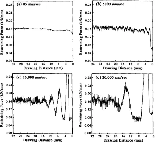
2.1.1. Pseudo drawing velocity for simulations. The experimental drawing velocity of 85 mm/sec and the pseudo velocities of 500 mm/sec, 5000 mm/sec, 10 000 mm/sec, 20 000 mm/sec and 30 000 mm/sec were examined to determine a reasonable simulation velocity. The radii of both the bead and groove shoulders were 5.5 mm, and the thickness of sheet metal was 0.86 mm. A Coulomb's coefficient of friction of 0.1 was assumed for the simulations, and the restraining forces were computed for each velocity. The simulation results for velocities of 85 mm/sec, 5000 mm/sec, 10 000 mm/sec and 20 000 mm/sec are shown in Fig. 2(a), (b), (c) and (d), respectively.
As seen in Fig. 2(a), the simulation reaches the steady state very soon with the low simulation speed. The curve obtained is very smooth and the restraining force of 0.162 kN/mm can be easily determined from the figure. As the simulation speed increases, the curve of the restraining force versus the drawing distance starts to oscillate. Figure 2(b) shows the computed curve of the restraining force obtained with the simulation speed of 5000 mm/sec. The value of the restraining force at the steady state, which is about the same as that obtained for 85 mrn/sec, can be determined easily despite the existence of a small amount of oscillation. When the velocity is increased to 10 000 mrn/sec, the ampli- tude of the oscillation becomes larger as shown in Fig. 2(c). However, a steady-state condition is still observed, but the value of the restraining force at the steady state is not so easily obtained as that in Fig. 2(a) and Fig. 2(b). A steady state is not obtained for the
0.28 I~ 0.24 Z 0.20 ~ 0.16 0 ee 0.12 .E (a) 85 mm/sec 0.08 0.04 0.00 32 2~8
2', 2'o
;2
;
0
D r a w i n g D i s t a n c e (mm) o.28 (b) 5000 mm/sec 0.24 Z 0.20 g. i ~ 0.12 o.os 0.04 0.00 1'2 ' ' 32 28 24 20 16 8 4 0 D r a w i n g D i s t a n c e (mm) B 0-28 t (c) 10,000 mm/sec I 0.28 (d) 20,000 m m / s e c ] / ~ 0"24 t | ~ ~ ~ 0.24 Z 0 . 2 0 ~ ~ 0.20 8 o.t~ ~ o.~6 o.o8 t o.os 0.04 t ~ 0.04 0 . 0 0 [ , , ' ' • , , i J 0.0C , , J , , 32 28 24 20 16 12 8 4 0 32 28 24 20 16 ;2 '8 4 0 D r a w i n g D i s t a n c e ( m m ) D r a w i n g D i s t a n c e (ram)Fig. 2. Restraining forces versus drawing distance with varied simulation speeds: (a) 85 mrrdsec; (b) 5000 mndsec; (c) 10 000 mm/sec; (d) 20 000 mm/sec.
Analysis o f an equivalent drawbead model 413 velocity of 20 000 mm/sec as in Fig. 2(d), since the restraining force in this case oscillates with a very large amplitude.
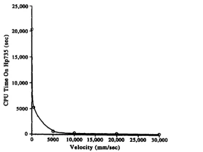
The C P U time consumed for the simulations for the various velocities is shown in Fig. 3. It can be seen in this figure that the C P U time is drastically reduced from 20 480 sec to 577 sec as the simulation velocity is increased from 85 mm/sec to 5000 mm/sec, and not m u c h advantage is gained by using velocities higher than I0 000 mm/sec. Taking both the accuracy of the restraining force computed and the C P U time consumed into consider- ation, the pseudo velocity of 5000 mm/sec seems to be a reasonable value to be used in the simulations for calculating the restraining force exerted by the real drawbead. 2.2. Optimum mesh systems
Since the critical time step (AT) is a function of the size of the minimum element in the assumed mesh for the sheet metal, the mesh size plays an important role as far as the computation time is concerned. However, the element size should not be so large as to reduce the accuracy of solution, especially for the sheet metal passing through the die surface which contains abruptly changed geometries or small comer radii such as draw- beads. In the finite element simulations, the drawbeads are treated as rigid bodies. The mesh system constructed for the drawbead is then used to define the geometry of the drawbead only, and is not involved in the computation of the sheet-metal deformation. Hence, a relatively small size of elements is necessary to describe the geometry of the drawbead as closely as possible to the actual one, so that the bending effects at the circular arc can be more accurately estimated. As far as the computation time is concerned, the number of elements for the drawbead only affects the contact-searching time, which is small compared with the computation time for the deformation calculation.
In the present study, optimum meshes for both the drawbead and the sheet metal are determined. The restraining force and the hold-on force computed using the proposed meshes are compared with the experimental and theoretical results.
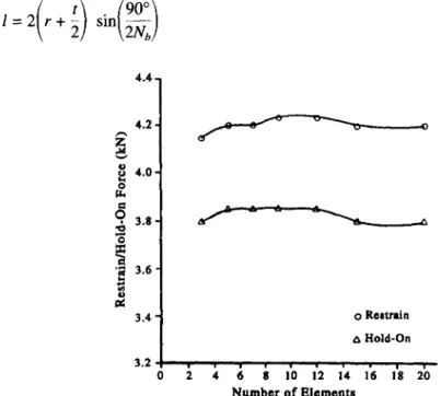
2.2.1. Mesh system for drawbeads. One half of the semi-circular head of the drawbead (or the groove shoulder) with a circumferential angle of 90 ° was taken as a unit for analy- sis. Seven different cases in which the unit circular arc is divided into 3, 5, 7, 8, 12, 15 and 20 elements, respectively, were examined, and the number of elements in the quarter circle was denoted by N d. Figure 4 shows the mesh system for the case of Nd=7. The other simulation data are as follows.
25,000" 20,000. o o'} r- 15,000- e l 0 o Ill 10,000 • 51111O. 0 . ~ 0 5000 10.000 15,000 20,000 25,000 30,000 Velocity (mmls~)
414 Fuh-Kuo Chen and Jia-Hong Liu
Fig. 4. Mesh system for the drawbead (Nd=7).
(a) The radius for both the bead and the groove shoulder is 5.5 cm.
(b) The sheet blank is made of AKDQ steel 100 mm long and 0.86 mm thick. (c) The number of elements for the sheet blank is 200.
(d) The coefficient of Coulomb's friction is 0.1.
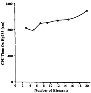
The restraining force and the hold-on force obtained from the simulations are shown in Fig. 5. It can be seen in Fig. 5 that both forces reach a steady value when Nd>--9. For the CPU time consumed for each case, as shown in Fig. 6, the difference is not so signifi- cant. Hence, in order to describe the geometry of the drawbead as closely as possible, a large value of Nd, such as 15, is recommended for the mesh used in the simulation.
2.2.2. Mesh system for sheet metal. The considered quarter circle of the bead was also used as the referenced unit for the sheet blank in the simulations. The accuracy of the deformation analysis depends very much on the value of the radius of the drawbead. The length of the element (l) for the sheet blank, as shown in Fig. 7, is calculated by the equation given below:
(1)
4.4- o O e~ o "O 4.2 4.0 3.8 3.6 3.4 3.2 0 ~ ; o Restrain Hold-On;
~ i'0 ;2 1'4 i'~ !'8 5b
Number o f ElementsAnalysis of an equivalent drawbead model 415 1200 v ' l m o u 800, 400- 0 N u m b e r of Elements
Fig. 6. CPU time consumed for different mesh systems of drawbead.
sheet-metal,
L
/-
Fig. 7. The length of element (l) for the sheet metal.
where r is the radius of the bead, t is the thickness of the sheet blank, and N b is the number of elements equally dividing the unit arc. Different drawbead radii (r) and sheet blank thicknesses (t), which were expected to have an influence on the simulation results, were analyzed and classified into four cases:
case (a): r=-5.50 mm, t=0.86 mm; case (b): r=4.75 mm, t=0.86 mm; case (c): r---4.00 mm, t=0.80 mm; case (d): r=-3.00 mm, r--0.80 ram.
The material for the sheet blank is still the AKDQ steel 100 mm in length, the coef- ficient of friction at the interface between the sheet blank and the dies is 0.1, and the number of elements used for the bead and groove shoulder is Nd=15 for all the four cases simulated.
4 1 6 F u h - K u o C h e n and J i a - H o n g L i u
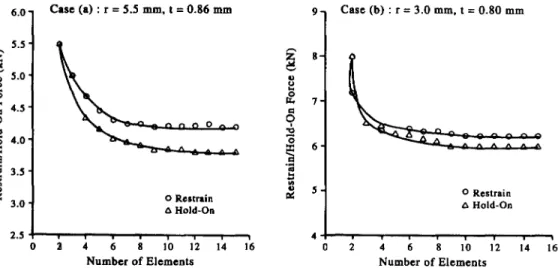
and case (d), as shown in Fig. 8(a) and (b), respectively, indicate that a steady-state value is reached when Nb>--8 for the two cases. The CPU time spent for case (a) increases exponentially with the number of the elements used for the sheet blank, as shown in Fig. 9. The other three cases possess the same trend as case (a) for the CPU time consumed versus the number of elements used for the sheet metal. In order to obtain an acceptable restraining force within a reasonable CPU time, an optimum number of elements, such as Nb=8, is recommended.
2.3. Experimental and theoretical validations
The validity of the optimum pseudo drawing velocity and mesh sizes for both the draw- bead and the sheet blank obtained from the above analyses were examined by the available experimental results [8] and the theoretical model [9]. The drawbead shape used in the simulations is similar to that shown in Fig. l(a). The four different cases listed below were simulated to obtain the restraining force using the optimum simulation parameters:
case (a): r=5.50 mm, t=0.76 mm, Nd=15, Nb=10; case (b): r=5.50 ram, t=0.86 mm, Nd=15, Nb=10, case (c): r----4.75 mm, t=0.76 mm, Nd=15, Nb=8; case (d): r---4.75 mm, t=0.86 mm, Nd=15, Nb=8; 5 . 5 ' A ~ 5.0' 0 ,., 4.5' O 4 . 0 . ~ 3.5' 3 . 0 ' 9 C a s e (b) : r = 3.0 m m , t = 0 . 8 0 m m o Restrain Hold-On ~, 7- o 6 143 ee~ t,~ Q [,.. 6.0' C a s e (a) : r = 5.5 m m , t = 0 . 8 6 mm 0 Restrain Hold-On 2.5 4 0 i ; 1'0 1'2 1'6 0 ; 1'0 1'2 l', 1'6
Number of Elements Number of Elements
Fig. 8. R e s t r a i n i n g force a n d h o l d - o n force for different d r a w b e a d radius (r) a n d sheet t h i c k n e s s (t): case (a) r=-5.5mm, t=0.86 m m ; case (d) r=-3.0 m m , t=0.80 mm. 4 0 0 0 - 3000- 2000 - 1000 0 2 4 6 8 1'0 1'2 1'4 1'6 Number of Elements
Analysis of an equivalent drawbead model 417 where r is the radius of the drawbead, t is the material thickness,
Nd
is the number of elements for drawbead, andNb
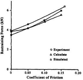
is the number of elements for sheet blank. The simulation drawing velocity in all these four cases is 5000 nurdsec. For each case, four different friction coefficients p,=0, 0.05, 0.1 and 0.15 were simulated so that the results could be compared with the experimental and theoretical values. The restraining force obtained from the simulation results of case (b), which is the medium value in these four cases, is compared with the experimental and the theoretical values, as shown in Fig. 10. As seen in Fig. 10, the computed values agree very well with both the experimental data and the theoretical predictions. As for case (a), case (c) and case (d), similar agreements are observed. The hold-on forces obtained from the simulations and experiments were also compared for each case, and the comparison between case (b) and the experimental data is shown in Fig. 11. It is seen in Fig. 11 that the computed values are smaller than the experimental values for the low friction, and higher than the experimental values for the higher friction. However, the difference is not significant.The simulation results also show that the friction between the drawbead and sheet blank has a significant effect on the restraining force. The fraction of the restraining force due to the friction to the total restraining force increases with the coefficient of friction non- linearly, and is in agreement with Nine's model.
The good agreements in the above comparisons of the simulated results with both the experimental data and the theoretical predictions indicate that the optimum pseudo drawing
6 ¢/J "7
y
0 E x p e r i m e n t A Calculate n Simulatedo o.~5 o.~o' o.;s 0.20 '
Coefficient of Friction
Fig. 10. Comparison of simulated drawing force with the experimental and theoretical values for case (b).
6.
m
o,
2. o Experiment
o Simulated
o o.bs o~io o.'~5 o.~o
Coefficient of Friction
418 Fuh-Kuo Chen and Jia-Hong Liu
speed and the mesh sizes for both the drawbead and sheet metal provide an efficient simulation for calculating both the restraining force and the hold-on force produced by the actual drawbead.
3. EQUIVALENT DRAWBEAD MODEL
As mentioned in the previous section, the computation time will be very large if the real drawbead shape is used in the finite element simulation. Therefore, an equivalent drawbead model is widely adopted to substitute for the real drawbead. In the equivalent drawbead model, the curved geometry of the drawbead is replaced by a flat surface, as shown by the shaded area in Fig. 1 (b). The restraining force produced by a unit width of the real drawbead during the stamping process is calculated using the same finite element program, following the procedures described in Section 2. The calculated restraining force is then assigned to the nodal points of the mesh constructed for the fictitious flat surface, according to the virtual work principle.
A simple method of examining the validity of the equivalent drawbead model is to check if the pulling force is the same as that obtained using the real drawbead shape in the setup, as shown in Fig. 12. The radius of both the bead and the groove shoulder is 5.5 mm. The AKDQ sheet metal with stress-strain relation 6"= 516e °23 MPa is used for the simulations. The length, width and thickness of the sheet metal are 100 mm, 4 mm and 0.86 mm, respectively. The element length for the sheet metal is 0.93 mm, which corresponds to Nb=10, and the number of Nd is chosen as 15 to construct the mesh of the drawbead. The coefficient of friction between the tooling and sheet metal is assumed to be 0.1 and the blank-holder force is 1.25 kN.
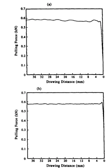
In the simulation with the real drawbead, the blank-holder moves down first to deform the sheet metal at the bead area and then clamps the sheet metal at the hold-on position. Subsequently, the sheet metal is pulled inward. The same die operations are applied to the simulation with the equivalent drawbead model, except that the sheet metal is not bent at the equivalent drawbead. The drawing forces at different punch strokes for simulations with both real and equivalent drawbeads are shown in Fig. 13(a) and (b), respectively. It is seen from Fig. 13(a) and (b) that the drawing forces at the steady state agree with each other very well with values of 0.58 kN and 0.57 kN, respectively. The CPU time con- sumed on an HP-735 workstation is 1013 sec for the simulation with the actual drawbead, and 45 sec for the simulation with equivalent drawbead, the latter being about one-twenti- eth of the former. The accuracy of the simulation results and the large saving in CPU time show the efficiency of using the equivalent drawbead instead of the real drawbead shape for the finite element simulations.
A further validation was performed by comparing the experimental data obtained by Wang et al. [9] with the finite element simulation results using the equivalent drawbead model. In the experiments, the relations between the clamping force exerted by the blank- holder and the punch load were determined for four different drawbead shapes used in a
I
F b!
2~Fe
Fe
I
T
l
- - P u l l i n g f o r c eAnalysis of an equivalent drawbead model 419 o eJ 0.'7 0.6 0.3 0.4 0.3 0.2 0.1 0 0.7 0.6 0.5 0.4 0.3 0.2 0.I 0 (a) I I I i I I I I I 36 32 28 24 20 16 12 8 4 0
Drawing Distance (ram)
(b)
I I I i I I I I I
36 32 28 24 20 16 12 8 4
Drawing Distance (ram)
Fig. 13. Pulling forces obtained from the simulations: (a) with real drawbead; (b) with equivalent drawbead model.
simple stamping process. Among the four drawbeads, the stamping process with the round bead, as shown in Fig. 14, was analyzed by the finite element simulation. The sheet blank is made of Fe/Zn electrogalvanized steel 0.73 mm thick with the mechanical properties as follows: the yield strength is 157 MPa, tensile strength is 302 MPa, work-hardening exponent (n) is 0.21, and the mean plastic-strain ratio (~) is 1.33. Since the stress-strain curve is not available in Ref. [9], the relation, ?r = 510~ "2~ MPa, which interpolates the mechanical properties of the sheet blank, was used in the finite element simulation. No lubricant was used in the stamping process except the mill oil which came with the sheet blank, and the corresponding coefficient of friction (/z) is about 0.2 as reported in [14]. However, simulation with coefficients of friction of 0.1, 0.15 and 0.2 were performed to examine the effect of friction.
The hold-on force (Hab) and the restraining force (Fib) for the drawbead were first calculated for the different frictional conditions as given below:
(a) for/a,=0.10, H~=52 N/ram, F~=55 N/mm; (b) for kr=0.15, Hdb=55 N/ram, Fdb=67 N/ram; (c) for/a=0.20, Hat----58 N/mm, Fdb'=75 Nlmm.
420 Fuh-Kuo Chen and Jia-Hong Liu
,,.- ~mm--~
Fig. 14. Stamping process with round beads [9].
punch travel of 63.5 mm was recorded. The punch forces at different clamping forces which were smaller than that caused a totally locked condition, for which the metal flow was prevented through the drawbead, were compared for those obtained from experiments and simulations, and the results are shown in Fig. 15. As seen in Fig. 15, the relations are linear, and the simulation results with/x---0.2 are the closest to the experimental data. This verifies that the equivalent drawbead model is applicable. It is also observed that the slopes of the straight lines increase with the increase of friction coefficient. This is not surprising because a larger punch force is required for a large value o f / x at the same clamping force to travel the same stroke.
300 -- "~ 2 0 0 - O ,d g ~. 100 - o Simulated It -- 0.20 Exp. by N. M. Wang 0 Simulated It = 0.15 O Simulated It -- 0.10 0 I I 0 200 400 C l a m p F o r c e ( N / r a m )
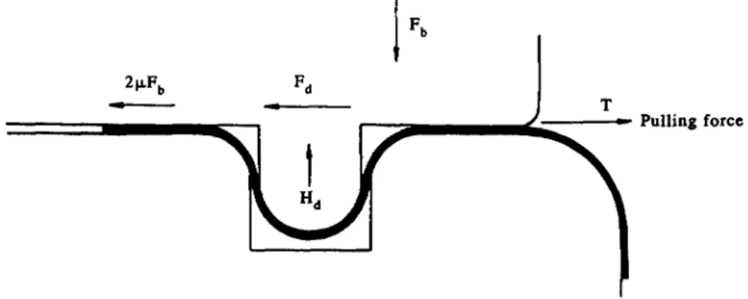
Analysis of an equivalent drawbead model 421 The relations between the slopes of straight lines shown in Fig. 15 and the values of tz can also be derived from the simple theoretical model depicted as follows. Figure 12 shows the free-body diagram for the forces involved in the stamping process. The free- body diagram is further simplified as shown in Fig. 16. For the force balance in the x direction:
o ~ r sin 0 d 0 = o ~ r j x cos 0 d0(2)+[Fd+2lx(Fb-Hd)]
and for the force balance in the y direction:
(2)
f-
2 Fso ~ r cos 0 d 0 +
-n-
o ~ r ~ sin 0 d 0 = F p . (3)
The punch force is then obtained from Equation (1) and Equation (2) as
1 + ~
Fp = 1--~ [Fa + 21x(Fb-Ha)]
(4)where F~ is the contact force exerted by the groove shoulder,
Fd
is the restraining force of the drawbead,Fb
is the total blank-holder force,Ha
is the hold-on force exerted by thedrawbead, and Fp
is the punch drawing force. For the condition Fb larger thanHa, Fb
isindependent of both
Fd and Ha,
and differentiating Equation (4) withFb
yields/1
+m=bFb= ,~l.~_~}
(5)where m is the slope of the straight lines shown in Fig. 15.
In the comparison of the theoretical values and the finite element results by plotting
F d + 21~
(Fb-H
d)
---allY
NTf437:4-B
Fp Fig. 16. Free-body diagram for pulling force calculation.
422 Fuh-Kuo Chen and Jia-Hong Liu | . 0 ~
/
m 0.5-- / / - - " -- ory / / ,no 0 : Simulation 0 I I I I 0 0.1 0.2 0.3 ItFig. 17. Relations between m and/x for a simple stamping process.
the relation of m and /z as shown in Fig. 17, the finite element results agree with the theoretical predictions very well. This fact once again lends support to the equivalent drawbead model.
4. SUMMARY AND CONCLUDING REMARKS
The three-dimensional finite element simulations for the stamping process using the equivalent drawbead model were studied in this investigation. In the equivalent drawbead model, the mesh for actual drawbead was replaced by a regular mesh to avoid relatively small elements used in the simulation. A systematic approach was proposed to compute the restraining force exerted by the actual drawbead, which was assigned to the mesh for the equivalent drawbead, using the finite element method. An optimum pseudo drawing speed and mesh systems for both the actual drawbead and sheet blank used in the compu- tation of the restraining force were determined through the proposed approach, resulting in a large saving in computation time. The calculated restraining force was confirmed by both the theoretical predictions and the experimental data published in the literature.
The equivalent drawbead model was examined by the published experimental data obtained in a simple drawing process. The punch forces obtained from the finite element simulations using the equivalent drawbead model were in good agreement with those obtained from experiments. A theoretical model was also proposed to predict the punch force. The predicted values showed a similar trend to that computed by the finite element simulations.
The computation time saved by the use of equivalent drawbead instead of the actual drawbead shape in the finite element simulations depends on the number of total elements used in the mesh system. However, for the simulations within a reasonable accuracy range, the computation time using the equivalent drawbead can be about one-twentieth of that with the use of the actual drawbead shape. The more complex the shape of the stamped part, the larger is the achievable saving in computation time.
Acknowledgements--The authors wish to thank the National Science Council of the Republic of China for their grant NSC-82-0422-E002-421 which made this project possible.
REFERENCES
[1] M. Gotoh, A finite element analysis of the rigid-plastic deformation of the flange in a deep-drawing process based on a fourth-degree yield function, International Journal of Mechanical Sciences 22, 367-377 (1980). [2] C. H. Toh, Y. C. Shiau and S. Kobayashi, Analysis of a test method of sheet metal formability using the
finite element method, Journal of Engineering in Industry 108, 3-8 (1986).
Analysis of an equivalent drawbead model 423 of planar anisotropic sheet metals and applications, International Journal of Mechanical Sciences 28(12), 825-840 (1986).
[4] S. Aim, E. L. Khaldi, L. Fontaine, T. Tamada and E. Tamnra, Numerical simulation of a stretch drawn autobody: Part I--assessment of simulation methodology and modelling of stamping components. SAE Paper No. 920639.
[5] S. Aim, E. L. Khaldi, L. Fontaine, T. Tamada and E. Tamura, Numerical simulation of a stretch drawn antobody: Part II--validation versus experiments for various holding and drawbead conditions. SAE Paper No. 920640.
[6] E. Hang and E. Di Pasquale, Industrial sheet metal forming simulation using explicit finite element methods.
Proc. Int. VD! Conf., Zurich, May, 1991.
[7] S. C. Tang, Quasi-static analysis of sheet metal forming processes--a design evaluation tool, Journal of Materials Processing Technology 45, 261-266 (1994).
[8] H. D. Nine, The applicability of Conlomb's friction law to drawbeads in sheet metal forming, Journal of Applied Metal Working 2(3), 200-210 (1982).
[9] N.M. Wang and V.C. Shah, Drawbead and performance, Journal of Materials Shaping Technology 9, 21- 26 (1991).
[10] N. M. Wang, A mathematical model of drawbead forces in sheet metal forming, Journal of Applied Metal Working 2(3), 193--199 (1982).
[11] N. Triantafyllidis, B. Maker and S. K. Samanm, An analysis of drawbeads in sheet metal forming: Part I--problem formulation, Journal of Engineering Materials Technology 108, 321-327 (1986).
[12] B. Maker, S. K. Samanm, G. Grab and N. Triantafyllidis, An analysis of drawbeads in sheet metal forming: Part II---¢xperimental verification, Journal of £ngineering Materials Technology 109, 164-170 (1987). [ 13] H. D. Nine, New drawbead concepts for sheet metal forming, Journal of Applied Metal Working 2(3), 185--
192 (1982).
[14] T. A. Hylton, C. J. Van Tyne and D. K. Matlock, Friction behavior of electrogalvanized sheet steels. SAE Paper No.930809.
![Fig. 14. Stamping process with round beads [9].](https://thumb-ap.123doks.com/thumbv2/9libinfo/8777903.214486/12.783.261.523.84.525/fig-stamping-process-round-beads.webp)
