臺灣高血壓疾病負擔及其對經濟成長的影響

全文

(1)國立臺灣大學公共衛生學院公共衛生學系學士班學生論文 Department of Public Health College of Public Health. National Taiwan University Bachelor Degree Thesis. 臺灣高血壓疾病負擔及其對經濟成長的影響 Disease Burden of Hypertension and Its Impact on Economic Growth in Taiwan. 廖為謙 Wei-Chien Liao. 指導教授: 鄭守夏博士 Advisor: Shou-Hsia Cheng, Ph.D. 中華民國 109 年 4 月 April 2020.

(2) Acknowledgment I would like to express my sincere gratitude to my advisor Professor Cheng, Shou-Shia for giving me great advice and idea on my thesis. It would be very difficult to complete my thesis without his mentoring. Besides, I would like to thank my thesis committee: Prof. Yang, MingChin and Prof. Lien, Hsien-Ming for their insightful comments and encouragement. My sincere thanks also go to Lin, Yi-Chieh for helping me get familiar with the NHI database. Last but not least, I would like to thank my family. Thank my parents, Liao, Chun-Hao and Chen, Ching-Ssu for unconditional support on my studies and living. This is my first time using the NHI database and trying to link the relationship between public health and macroeconomics. It is a splendid experience for me to learn how to find useful data from a large database, to construct a possible model with numerical analysis, and to reason the implication behind tables and graphs.. i.

(3) 國立臺灣大學學士班學生論文. 口試委員會審定書臺灣高血壓疾病負擔及其對經濟成長的影響 Disease Burden of Hypertension and Its Impact on Economic Growth Impact in Taiwan 本論文係廖為謙君（B05801010）在國立臺灣大學公共衛生學學系完成之學士班學生論文，於民國 109 年 04 月 23 日承下列考試委員審查通過及口試及格，特此證明. ii.

(4) iii.

(5) iv.

(6) 中文摘要高血壓為全球最嚴重的健康問題之一，卻鮮少有研究討論其產生的經濟影響。臺灣有完整的健保資料庫，卻不像美國對於高血壓失能患者有定期的做問卷調查。如何有效的測量高血壓的間接成本是值得探討的。本研究計算高血壓的疾病負擔與經濟損失，並利用人力資本法估算其對經濟成長的影響。針對經濟成長模型，本研究以 Grossman 的個體健康投資模型作為基礎發展的人力資本內生化的成長模型。結果顯示在 2001 到 2017 年間，高血壓疾病的直接成本不斷上升，尤其是藥費的增長；若罹病時間增長，則直接成本的增長幅度也越大。發生率與急診住院的人數有稍微下降。至於成長模型的迴歸分析方面，疾病的影響並不顯著。從研究中發現，雖然高血壓的疾病影響，對於總體經濟的影響並不顯著，但從成本法去估算仍然有很大的疾病負擔，從數值分析去模擬改變對健康的投資行為時，可以見到健康與經濟成長的關係與個體對健康的投資的外溢效果，未來值得對健康與經濟發展建立更嚴謹的理論模型。. 關鍵詞: 高血壓, 經濟成長, 疾病負擔, 間接成本, 健康經濟. v.

(7) Abstract Hypertension has been one of the most serious health conditions in the world, but few studies have captured its economic impact. Taiwan has an advantage on the NHI database which is highly representative; however, unlike the U.S., Taiwan does not conduct regular surveys to measure the disability of hypertensive and cardiovascular patients. The tools to measure the cost of diseases especially the indirect cost is worth of investigation. This study calculated the disease burden of hypertension and estimated its impact on economic growth by using the human capital method. For the economic growth model, an endogenous human capital growth model founded on a modified version of the Grossman model is considered. The results show that the direct cost is increasing, especially the drug expenses. We found that the longer the duration of hypertension the larger the growth rate of direct costs. The incidence and the number of patients visiting an emergency department or hospitalized decreased slightly over the 17 years. As for the regression model for the economic growth, the disease factor for hypertension is not significant. However, the results show a heavy disease burden of hypertension, especially its drug expenses. Given that the disease factor in the economic growth model is not significant, it shows significant relationship between the health and the economic growth in the simulation models. Further study to construct an advanced and robust model describing the relationship between health and economic growth is recommended.. Keywords: Hypertension, Economic Growth, Disease Burden, Indirect Cost, Health Economics. vi.

(8) Contents Acknowledgment…………………………………………………………………………………..i 口試委員審定書………………………………………………………………………………….ii 國立臺灣大學行為與社會科學研究倫理委員會審查核可證明………………………………iii 國立臺灣大學行為與社會科學研究倫理委員會行政變更審查證明…………………………iv 中文摘要………………………………………………………………………………………….v Abstract...……………………..…………………………………………………………………..vi Contents ..……………………..…………………………………………………………………vii 1. Introduction ............................................................................................................................. 1 2.. Literature Review.................................................................................................................... 1 2.1.. Related Researches in the U.S.......................................................................................... 1. 2.2.. Related Researches in Taiwan .......................................................................................... 2. 2.3.. Reduction of productivity for hypertension patients ........................................................ 3. 2.4.. Labor force loss from mortality ....................................................................................... 4. 2.5.. Caregiver Cost Estimation ............................................................................................... 4. 2.6.. Hypertension issue in Economic Growth ......................................................................... 5. 3.. Research Objective ................................................................................................................. 6. 4.. Study Design ........................................................................................................................... 7 4.1.. Hypertension .................................................................................................................... 7. 4.2.. National Health Insurance Database (NHID)................................................................... 7. 4.3.. Estimation of Hypertension disease burden ..................................................................... 8. 4.3.1.. Incidence ................................................................................................................... 8. 4.3.2.. Mortality ................................................................................................................... 8. 4.3.3.. Disability-adjusted life years (DALY) ...................................................................... 9. 4.3.4.. Direct Economic Costs ............................................................................................. 9. 4.3.5.. Indirect Economic Costs ......................................................................................... 10. 4.4. 5.. Economic growth model ................................................................................................ 12. Results ................................................................................................................................... 16 5.1.. Cost Method ................................................................................................................... 16. 5.1.1.. Incidence, Mortality, and DALY ............................................................................. 16. 5.1.2.. 2001 Cohort Follow-up ........................................................................................... 18. 5.1.3.. New cases cross-sectional from 2001 to 2017 ........................................................ 19. 5.1.4.. The Result of the Simulation .................................................................................. 22. 5.1.5.. The Result of the Regression Model ....................................................................... 24. 6.. Discussion ............................................................................................................................. 25. 7.. Limitation.............................................................................................................................. 27 vii.

(9) 8.. Conclusion ............................................................................................................................ 28. Reference ...................................................................................................................................... 30 Appendix A. The Lagrange Methods for the Simulation .............................................................. 32 Appendix B. Graphs...................................................................................................................... 33 Appendix C. NHID Application Form .......................................................................................... 35. List of Figures Figure 1 Incidence by age group ................................................................................................... 17 Figure 2 Mortality by age group ................................................................................................... 17 Figure 3 Total direct cost (cohort from 2001) ............................................................................... 18 Figure 4 Total indirect cost (cohort from 2001) ............................................................................ 18 Figure 5 Average direct cost among male (cohort from 2001) ..................................................... 19 Figure 6 Average direct cost among female (cohort from 2001) .................................................. 19 Figure 7 Total indirect cost (cross-sectional) ................................................................................ 21 Figure 8 Total direct cost (cross-sectional) ................................................................................... 21 Figure 9 Average direct cost among male (cross-sectional) ......................................................... 21 Figure 10 Average direct cost among female (cross-sectional) .................................................... 21 Figure 11 Total drug expense (cross-sectional) ............................................................................ 22 Figure 12 Total drug expense (cohort from 2001) ........................................................................ 22 Figure 13 Change in leisure time .................................................................................................. 23 Figure 14 Change in consumption ................................................................................................ 23 Figure 15 Change in capital investment........................................................................................ 23 Figure 16 Change in health time investment ................................................................................ 23 Figure 17 Change in working hours.............................................................................................. 24 Figure 18 Change in health capital investment ............................................................................. 24 Figure 19 Average indirect cost among male (cohort follow from 2001)..................................... 33 Figure 20 Average indirect cost among female (cohort follow form 2001).................................. 33 Figure 21 Indirect cost among female (cross-sectional) ............................................................... 33 Figure 22 Indirect cost among male (cross-sectional) .................................................................. 33 Figure 23 Average drug expense per person (cross-sectional) ...................................................... 33 Figure 24 Average drug expense per person (cohort follow from 2001) ...................................... 33 Figure 25 The ratio of IPD over OPD ........................................................................................... 34 Figure 26 Emergency bed day ...................................................................................................... 34. List of Tables. Table 1Incidence, Incidence proportion, and Mortality ................................................................ 17 Table 2 YLD, YLL, and DALY .................................................................................................... 17 Table 3 Total Direct and Indirect Cost .......................................................................................... 20 Table 4 The coefficients of the regression model ......................................................................... 25. viii.

(10) 1. Introduction Hypertension is now a serious health condition with more than 1.13 billion people are suffering from hypertension1 (World Health Organization, 2020). Although the syndromes are vague and most people are neglect, it may lead to many serious cardiovascular diseases, such as stroke, hypertensive heart disease, heart failure, and so on. These diseases would cause huge medical costs and last for a long time (Chodick, et al., 2010). In Taiwan, hypertension has been reported to be one of the diagnoses with very high drug expenses (衛生福利部健康保險署, 2010). Although hypertension poses a heavy burden for many developed countries, few studies have measured its disease burden or economic impact. For those studies who discussed disease burden of hypertension, most of them focus on the U.S., and very few studies using Taiwan’s data. The common approach to estimate the disease burden is to estimate the prevalence, mortality, and DALY (Kay, Pruss, & Corvalan, 2000). Yet, to assess the efficiency or effectiveness of the policy, most studies would assess the burden by measuring the economic impact of the disease. Therefore, to calculate the direct and indirect cost precisely for hypertension and to compare the different methods would be the main target of this study.. 2. Literature Review 2.1.. Related Researches in the U.S.. To measure the economic impact of the disease, the common way of measurement includes the direct cost of medical cost, and the indirect cost by applying the human capital approach. The medical expenditure includes outpatient visits, inpatient visits, emergency visits, and drug fees 1. 25% of men and 20% of women are suffered from hypertension in 2015 according to the WHO website. 1.

(11) (American Diabetes Association, 2008). As for the indirect cost, most studies include productivity loss from getting the disease (sick leave and mental problems), working hour loss due to the demand for caregiving, productivity loss due to mortality. The previous U.S. studies usually refer the disabled weight to the past survey for Activities of Daily Living (ADL) or other working ability surveys that assessing the impairment of the patient suffers from hypertension. Then, they matched age and sex to project the whole patient population status of working ability. In this study, several coefficients of the disabled weight of hypertension were adopted from those studies, while others were estimated for Taiwan cases.. 2.2.. Related Researches in Taiwan. Taiwan is known for its comprehensive and high-quality National Health Insurance Database. To estimate the health expenditure, there is no need to do sampling but use the whole patient population. Yet, there is no regular worker impairment survey every year. This makes it quite easy to estimate the direct cost but hard to estimate the indirect cost especially for the loss of productivity of labor and loss working hour due to caregiving demand. One study has been conducted to estimate the economic impact of enterovirus infection in Taiwan in 2015. The study streams the dataset of inpatient visits, outpatient visits, emergency visits, drug fees, and hospital stays to measurement the disease burden of enterovirus (Liu, et al., 2015). To estimate the economic impact, the direct cost of medical expenditures was calculated, and indirect cost includes travel costs, productivity loss of caregivers, and costs associated with premature mortality of patients are estimated by a human capital method. Yet, there are several differences between this enterovirus study and the hypertension study. First, the enterovirus is an acute disease. The syndrome would appear soon and is easy to be detected, which makes the cost is easy to be estimated. On the other hand, hypertension is a 2.

(12) chronic condition, which has a strong potential to cause other cardiovascular diseases but is hard to estimate the cost. Second, the target population of the enterovirus is children, there is no need to consider the production loss from the disease and children would need their parents to take them to see a doctor. However, in the hypertension case, the production loss of workers due to the there are a bunch of patients above age 15 must be estimated. Moreover, it is hard to estimate the loss of production due to caregiving since patients are capable to go to see a doctor by themselves.. 2.3.. Reduction of productivity for hypertension patients. To calculate the cost of sick leaves, Arno calculates days of sick leaves and multiplies with average earnings by specific age per day. The cost of caregivers taking leaves is calculated by days that patients are hospitalized or stay in ICU multiplied by average earnings for a worker in Taiwan. The reduction in productivity caused by hypertensive diseases is measured by the difference between earning of normal workers and hypertension workers multiplied with remaining life years (Arno, Levine, & Memmott, 1999). To estimate the production loss of hypertension patients, most studies reviewing the survey on the elderly health status or ADL. Yet, according to the study from Hu, the loss of ADL caused by hypertension is not significant (Hu, Hu, Hsu, Hsieh, & Li, 2012). Therefore, in this study, the direct production loss from hypertension would not be calculated into the indirect cost but those derivative acute diseases. According to the traditional cost-effectiveness analysis, one can measure the cost by adding up the cost of all the conditions that the disease may occur (here is hypertension) (Muennig, 2007). If there are more syndromes, then the highest cost of chronic disease should be seen as the dominating one. Types of indirect costs often include loss of productivity from morbidity and 3.

(13) premature mortality. Morbidity costs often include work loss among individuals, home productivity loss, and work loss for too sick to work. To estimate work loss among individuals due to too sick to work, the paper from American Diabetes Association matches the demographic data and the patient data and takes sick leave as the indicator of too sick to work (American Diabetes Association, 2008).. 2.4.. Labor force loss from mortality. The definition of the labor force refers to those who are currently working and the age above 15 from the Ministry of Labor in Taiwan. To estimate the loss of the labor force from mortality, one uses the growth model to capture the impact (Kalemli-Ozcan, Ryder, & Weil, 2000) (Finlay, 2007). Few studies discussed the loss from mortality via the cost estimation (Goetzel, et al., 2004).. 2.5.. Caregiver Cost Estimation. Caregiving includes formal and informal caregiving. In Taiwan, people often hire immigrants from South-East Asia for caregiving, and the reasonable wage is about 2000 to 2400 NTD per day (The Reporter, 2020). On the other hand, informal caregiving considers those family members to come to the hospital and take care of patients. To estimate the caregiver cost, the guideline proposed by Arno, Levine, and Memmott (Arno, Levine, & Memmott, 1999) asking the following questions: (1) What is the national prevalence of informal caregiving? (2) What is a reasonable market wage that would have to be paid to replace informal caregiving? This study is not going to survey on Income and Program Participation, National Survey of Families and Households, National Health Interview Survey, or National Long-term Care Survey, but using the NHID to estimate the effect. From the estimation published by Labor 4.

(14) Ministry in Taiwan in 2015, there is one-fifth (2.31 million people) of the total workers (11.53 million people) in Taiwan are affected by informal caregiving (勞動部, 2010). Critics for the indirect cost include the comment from Abegunde that the indirect cost may mislead the truth because with the high unemployment rate, for those patients who take sick leaves or cannot work, their family will replace their place. Therefore, the economic impact would be overestimated. He argues that the economic growth model would be a more accurate method to capture economic impact (Abegunde, Mathers, Adam, Ortegon, & Strong, 2007).. 2.6.. Hypertension issue in Economic Growth. The economic growth model proposed by Solow as AK type model with share belongs to (0,1), such as: 𝑌 = 𝐴𝐾 𝛼 𝐿1−𝛼 (Solow, 1956) Y stands for the level of living, K stands for physical capital stock, L stands for the size of the labor force, A stands for the total factor productivity, 𝛼 stands for the share of physical capital stock. After 1980, there are many researchers analyze how to improve the endogenous problem in the model. For the endogenous growth model, the macro-growth model needs to stand on the foundation of a micro-representative individual optimal decision problem. One of the factors they want to capture is a labor-augmented factor such as human capital. Moreover, human capital includes education and health status. Kalemli took care of the human capital investment with increasing life expectancy. (Kalemli-Ozcan, Ryder, & Weil, 2000) There are more factors rather than life expectancy, but few health topics have been discussed in the economic growth. Finlay’s. 5.

(15) study proposed that education can affect health status. The model was adopted in a two-period utility maximization problem and considers the interaction with health and education (Finlay, 2007). Also, Chakraborty uses the economic growth model to examine the different health status groups that would reach a different equilibrium in the economy (Chakraborty, 2004). Cervellati constructs an overlapping generation model to capture the relationship between health and economic growth (Cervellati & Sunde, 2005). To combine these models above, it is reasonable to consider a stochastic process on losing their life, and the possibility for patients to occur hypertension follows Poisson Process. Also, to form the microeconomics foundation for Solow model, the model should consider (1) a two-period maximization problem (2) interaction between health and education (3) the medical expenditure (4) capital saving (5) fertility and mortality rate (6) the role of life expectancy and the disease weight.. 3. Research Objective This study consists of two sections. The first section calculates the hypertension disease burden and economic costs due to hypertension diseases. The second section measures the cost of hypertension diseases by using the economic growth model via the human capital method. The literature review has discussed the pros and cons of calculating the expenditure method and modeling the growth model method (Abegunde, Mathers, Adam, Ortegon, & Strong, 2007). Yet, for this paper, the specific disease in one country is discussed rather than the international comparison. The objective of this study is to estimate the economic impact of the disease burden of hypertension from 2001 to 2017 and to compare the result by using the two methods.. 6.

(16) 4. Study Design 4.1.. Hypertension. Hypertension discussed in this study refer to International Statistical Classification of Disease and Related Health Problems 10th Revision as essential hypertension (ICD10 I10), hypertensive heart disease (ICD10 I11), hypertensive chronic kidney disease (ICD10 I12), hypertensive heart and chronic kidney disease (ICD10 I13), secondary hypertension (ICD10 I15), and Hypertensive Crisis (ICD10 I16) in this study. Although hypertension is easy to be defined in clinical practice, it is hard to construct the causal relationship between hypertension and the specific economic cost. The relation is ambiguous because many diseases may cause hypertension by the immune system as secondary hypertension. Also, when it comes to complications, hypertension is usually considered as the least important disease.. 4.2.. National Health Insurance Database (NHID). National Health Insurance Database is highly representative since over 99.5 percent of Taiwan residents are covered by the National Health Insurance (National Health Insurance Administration, 2016). The study extracted the Registry for beneficiaries, Ambulatory care expenditures by visits, Inpatient Expenditures by Admissions, and Cause of Death Data from the Hypertension Health Database in the National Health Insurance Database. All patients are included in the database for three or more than three times a hypertension record (ICD9 401-405; ICD10 I10-I16) in the column of ICDCM_1, ICD9CM_2 or ICD9CM_3 in Ambulatory care expenditures by visit, and the period between each time should be longer than four weeks. (Manual of Hypertension Health Database). 7.

(17) 4.3.. Estimation of Hypertension disease burden. Although the economic impact is a crucial part of the paper, some disease burden indicators such as incidence, mortality, and Disability-Adjusted life years are calculated and presented in the paper. 4.3.1. Incidence One measures the point prevalence of hypertension residents in Taiwan every year from 2001 to 2017 from National Health Insurance Database data. To calculate the incidence proportion, this study uses the equation as below:. Incidence in 𝑦𝑒𝑎𝑟𝑖 = #𝑜𝑓 𝑛𝑒𝑤 𝑝𝑎𝑡𝑖𝑒𝑛𝑡𝑠 𝑖𝑛 𝑁𝐻𝐼𝐷 𝑤𝑖𝑡ℎ ℎ𝑦𝑝𝑒𝑟𝑡𝑒𝑛𝑠𝑖𝑜𝑛 𝑖𝑛 𝑦𝑒𝑎𝑟𝑖. (Bonita, Beaglehole, & Kjellstron, 2006) Also, stratified incidence proportion by age is going to be conducted.. Incidence proportion in 𝐴𝑔𝑒𝑖 in 𝑦𝑒𝑎𝑟𝑖. =. #𝑜𝑓 𝑛𝑒𝑤 𝑝𝑎𝑡𝑖𝑒𝑛𝑡𝑠 𝑖𝑛 𝑎𝑔𝑒 𝑖 𝑖𝑛 𝑁𝐻𝐼𝐷 𝑤𝑖𝑡ℎ ℎ𝑦𝑝𝑒𝑟𝑡𝑒𝑛𝑠𝑖𝑜𝑛 𝑖𝑛 𝑦𝑒𝑎𝑟 𝑖 𝑇𝑜𝑡𝑎𝑙 # 𝑜𝑓 𝑖𝑛 𝑎𝑔𝑒 𝑖 𝑖𝑛 𝑦𝑒𝑎𝑟 𝑖. 4.3.2. Mortality Mortality is an important indicator of the severity of the disease. As prevalence data is hard to obtain, mortality rather than mortality proportion is considered in this study. 8.

(18) 4.3.3. Disability-adjusted life years (DALY) Disability- Adjusted life years is one of the common indicators for disease burden. This is designed by the World Bank to assess the priority of health policy (CJ & AD, 1997). One DALY can be deemed as one-year loss from healthy life years. (World Health Organization, 2019) DALY consists of years of lost life (yLL) and years lost to disability (yLD). The calculation methods are as followed:. 𝐷𝐴𝐿𝑌 = 𝑦𝐿𝐿 + 𝑦𝐿𝐷. 𝑦𝐿𝐿 = #𝑜𝑓 𝑑𝑒𝑎𝑡ℎ 𝑖𝑛 𝑒𝑎𝑐ℎ 𝑎𝑔𝑒 × 𝑠𝑡𝑎𝑛𝑑𝑎𝑟𝑖𝑧𝑒 𝑙𝑖𝑓𝑒 𝑒𝑥𝑝𝑒𝑐𝑡𝑎𝑛𝑐𝑦 𝑎𝑡 𝑡ℎ𝑒 𝑎𝑔𝑒. 𝑦𝐿𝐷 = # 𝑜𝑓 𝑖𝑛𝑐𝑖𝑑𝑒𝑛𝑐𝑒 𝑟𝑎𝑡𝑒 × 𝑎𝑣𝑒𝑟𝑎𝑔𝑒 𝑑𝑢𝑟𝑎𝑡𝑖𝑜𝑛 × 𝑤𝑒𝑖𝑔ℎ𝑡 𝑓𝑎𝑐𝑡𝑜𝑟. In this study, the weight factor refers to the weight factor of hypertension states in the WHO website published in 2004 (World Health Organization, 2020) as 0.246. 4.3.4. Direct Economic Costs To calculate the economic costs caused by hypertension, this study changes all the costs from characteristic measurements to dollar unit. In this study, all the costs are presented in NT dollars. The study assesses direct costs and indirect costs caused by hypertension. Direct costs include medical expenditures, which includes registration fees, medication expenditures paid by health insurance, and copayments (Liu, et al., 2015). The department considers outpatient department visits (OPD visits) and inpatient visits (IPD visits), hospitalization, and drug 9.

(19) expenditure (Akobundu, Ju, & Mullins, 2006). Since over 99.5 percent of Taiwanese residents are covered by National Health Insurance and National Health insurance almost covers all the medical costs, the cost paid from out of pocket is relatively small. 4.3.5. Indirect Economic Costs2 Indirect costs are estimated by the human capital approach, including reduction of productivity for hypertension patients, labor force loss from mortality, and labor force loss from caregiving.. Reduction of productivity for hypertension patients. The reduction of productivity for hypertension patients consists of two parts. The first part is the absence of work due to sick leave; the other part is due to the reduction of marginal productivity. In the former part, sick leaves are counted as the record of hospital stay.. Cost of sick leaves = (Bed dayE + Bed dayS ) × Dep × I × Attributable Risk. I stands for the average salary the patients should pay for the insurance premium in the specific group. Dep is the indicator that records if the patients have a job. This is to make sure even the cost only calculated for those would originally have a job. In the second part, this study refers to the study conducted by Chang in 2011 that he argues stroke and coronal heart disease will increase the probability of becoming disability and mortality (張國維, 2011), but essential hypertension will not increase the probability of 2. Conducting Research on the Economics of Hypertension to Improve Cardiovascular Health 10.

(20) becoming disabled nor being dead. Therefore, the reduction of marginal productivity in this paper only includes stroke and hypertensive heart disease patients (ICD9 430-438; ICD10 I60I69; ICD9 402; ICD10 I11 ). Bed dayE stands for the number of emergency bed stay. Bed dayS stands for the number of chronic bed stay. Attribution to be hospitalized is 0.3511 (Ruiz-Hernandez, et al., 2018).. RMP in 𝑦𝑒𝑎𝑟𝑖 = # of patients occurs disease in 𝑦𝑒𝑎𝑟𝑖 × Discount Weight × Attributable Risk. Reduction Marginal productivity (RMP) equals to the number in specific syndrome times the discount weight and attributable risk. The discount weight here refers to the disability weight of year of the disabled losing year published on Institution for Health Metrics and Evaluation, which refers to 0.303 (Institute for Health Metrics and Evaluation (IHME), 2010) and For those stays ICD9 402 or ICD10 I11 patients, the discount weight would be 0.098. The attributable risk for stroke would be 0.233 and the ICD 402 is 0.3367 (Ruiz-Hernandez, et al., 2018).. Labor force loss from mortality. The labor force loss from mortality (LFLM) considers the potential labor force would devote to the labor market in the future. Therefore, how much patients can participate in the labor market in the future if they were not sick is crucial to be identified. To estimate the loss from mortality, the following statistics are going to be considered: (1) Taiwan’s life expectancy (L) (2) The age the patients died (A) (3)Taiwan’s labor participation rate stratified in different age groups (PR 𝑖 ) (4) Taiwan’s average wage (𝑊𝑖 ) in different age groups. (5) Attributable risk(w) 11.

(21) which is indicated to be 0.0843. LFLM = ∑(L − A) × PR 𝑖 × 𝑊𝑖 × w. Labor force loss from caregiving (LFLC). To estimate the demand of caregiver in the hospital stay and outpatient visit, this study considers (1) most of the children need their parents to bring them to hospital and take care of them when they stay in the hospital (2) patients who suffer from stroke need to ask their family member take them to the hospital and take care of them in the hospital, (3) the rest of the patients would not be calculated.. LFLC = ((Bed dayE + Bed dayS ) × I × C1 × 0.3367/30 + (OPDv + IPDv ) × I × C2 × 0.3511/30. C1 is 1 if the patients suffer from stroke or children; C2 is 1 if the patients are children.. 4.4.. Economic growth model. Considering the human capital accumulation model in the Solow growth model, one separates the total factor productivity (A) into technology progress as well as labor augmented health capital and education capital. One rewrites the production function as:. 𝑌 = 𝐴𝐹(𝐻, 𝐾, 𝐿). 12.

(22) 𝑌𝑡 = 𝐴𝑡 (ℎ𝑡 𝐸𝑡 𝐿𝑡 )𝛼 𝐾𝑡1−𝛼. Y is the total output, A is technological progress. H is the human capital which can be estimated by H= (E, h, t, …), h is the health capital, which would be affected by disease burden. t is the dummy variable for estimate time random effect. E is the education capital, which would be estimated by enrollment rates of colleges and universities in Taiwan. Since Taiwan enforces the 9-year compulsory education in 1968, it is meaningless to investigate the change in the enrollment rate in middle school. L is the size of the labor force, which is derived from the labor force population from the Ministry of Labor. K is physical capital, which can be determined by the national income equation. The law of motion for the variables follows: 𝐾𝑡+1 = 𝐾𝑡 (1 − 𝛿1 ) + 𝐼𝑘𝑡 𝐴𝑡+1 = 𝐴𝑡 (1 + g) 𝐿𝑡+1 = 𝐿𝑡 (1 + η). 𝛿 is the economic depreciation rate. 𝐼𝑘𝑡 is the investment in the physical capital. g is technological progress. η is the growth rate of the population. ℎ𝑡 =DALY The total factor indicator combines two different factors: technology and human capital. For human capital, it includes health capital and education capital. This study stands with the same view as Grossman, who proposed the health capital theory that people can decide whether to invest their health capital or not (Grossman, 1972). Furthermore, the study assumes health capital is constant-return-to-scale, so the study can attain society’s health capital by adding individual health capital. Another factor that affects human capital is education capital, which has often been measured by different indicators. The study assumes education capital can be 13.

(23) reflected by the enrollment rate of college and university in Taiwan. Although David N. Weil criticizes enrollment rate for reflecting only the quantity of education but not the quality of education, it is hard to find one normalized test lest for a long time and to compare test results (Weil, 2009). The production function fulfills the Solow assumption (Solow, 1956)that but without the assumption that α ∈ (0,1) : (1) the function is homogeneous of degree one (constant-return-to-scale) (2) 𝐹𝑖 = (K, L) > 0 (3) 𝐹𝑖𝑖 = (K, L) < 0 (4) 𝐹 = (0, L) = 0 (5) lim 𝐹𝑘 = (K, L) → ∞ ; lim 𝐹𝑘 = (K, L) → 0 𝑘→0. 𝑘→∞. For the parameters, s is the saving rate and 𝛼 is the factor share. Take the logarithm of the growth model, (𝑙𝑜𝑔𝑌𝑡 − 𝑙𝑜𝑔𝑌𝑡−1 ) = 𝛽0 + 𝛽1 log 𝑌𝑡 + 𝛽2 𝑙𝑜𝑔𝐴𝑡 + 𝛽3 𝑙𝑜𝑔ℎ𝑡 + 𝛽4 𝑙𝑜𝑔𝐸𝑡 +𝛽5 𝑙𝑜𝑔𝐿𝑡 + 𝛽6 𝑘𝑡 (Finlay, 2007) This equation would be used to estimate the coefficients. Different from the model proposed by Finlay, this model did not consider mortality as the endogenous factor of the growth of the labor market. Also, numerical simulation in the scope of a representative individual is considered in this study. To do so, consider a representative individual face an infinite horizon maximization problem adaptive from the Grossman health investment model (Grossman, 1972). In the study, the representative individual can not only decide whether to split her/his time to leisure or work. 14.

(24) but also engage in exercising as health investing. The maximizing problem is as follows:. max ∑ 𝛽 𝑡−1 𝑢(𝑐𝑡 , 𝑡𝑙𝑡 ) = 𝑢(𝑐1 , 𝑡𝑙1 ) + 𝛽𝑢(𝑐2 , 𝑡𝑙2 ) + 𝛽 2 𝑢(𝑐3 , 𝑡𝑙3 ) … 𝑠. 𝑡. Iℎ𝑡 + Ikt + ct = 𝑎𝑡 + 𝑤𝑡 𝑡𝑛 + (1 + 𝑟ℎ𝑡−1 )𝐼ℎ𝑡−1 + (1 + 𝑟𝑘𝑡−1 )𝐼𝑘𝑡−1 Iℎ𝑡 = 𝐺ℎ𝑡 + 𝐸𝑥𝑝ℎ 𝑡ℎ + 𝑡𝑙 + t n = ℎ𝑖 ∗ Ω ; Let ℎ𝑖 ∗ Ω = 1 𝑢(𝑐𝑡 , 𝑡𝑙𝑡 ) denoted the utility function for the representative individual. 𝛽 is the time 1. preference, follows 𝛽 = 1+𝑟. 𝑘𝑡−1. . Iℎ𝑡 is the investment for health capital. I𝑘𝑡 is the investment for. physical capital. ct is the consumption in period t. 𝑎𝑡 is the endowment in period t. 𝑤𝑡 is the wage level in period t. 𝑡𝑛𝑡 is the working hours in period t. 𝑟ℎ𝑡−1 stands for the return of health capital investment. 𝑟𝑘𝑡−1 stands for the return of physical capital investment. 𝑡ℎ 𝑡 stands for the time investment in health (healthy activities; exercising). 𝐺ℎ𝑡 is the marginal product of health capital. 𝐸𝑥𝑝ℎ stands for health care expenses. Ω represents the total time.. 15.

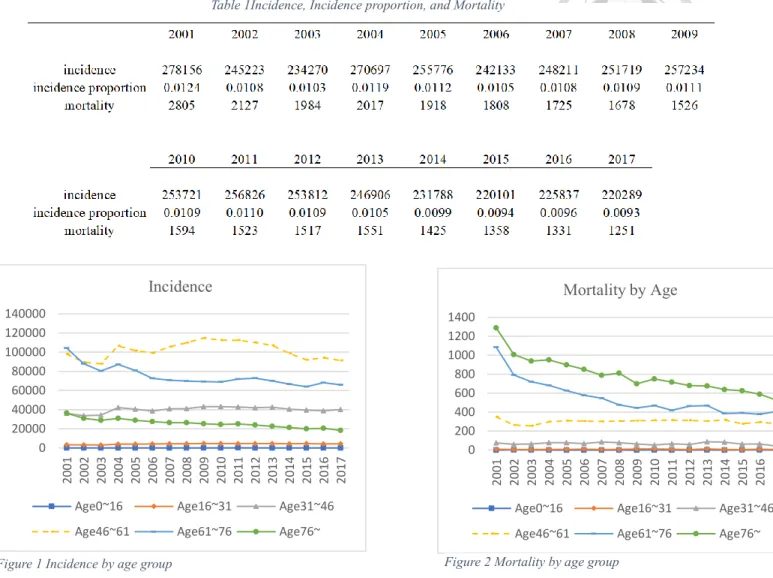
(25) 5. Results 5.1.. Cost Method. 5.1.1. Incidence, Mortality, and DALY The incidence is stationary at 250,000 new cases each year but has been slightly decreasing from 2014. The prominent change would be the age group 61-76, which has a large decrease over time. As for the mortality, the mortality is decreasing over time, especially for those groups above 61 years old. The trend of DALY is alike incidence. The average is 603891.4 health years. The good news is that YLL is decreasing over time from 41739.3 healthy years to 21373.9 healthy years. Compare to Japan and Korea, the DALY are 46,600 and 43,000. Taiwan is better; however, if one standardizes the population, the DALY is higher than Korea and Japan. Also, the YLD estimate here may be an overestimate. Comparing Taiwan YLD for hypertension to Korean and Japanese data, Korean is 17,000 healthy years and Japan is 63,700 healthy years. One possible reason may be the YLD here is more similar to the cardiovascular diseases YLD rather than hypertensive diseases. For Korean, cardiovascular diseases YLD is 269,600, and Japan is 1,157,200. Taiwan is still higher if the population size is considered.. 16.

(26) Table 1Incidence, Incidence proportion, and Mortality. Incidence. Mortality by Age 1400 1200 1000 800 600 400 200 0 2001 2002 2003 2004 2005 2006 2007 2008 2009 2010 2011 2012 2013 2014 2015 2016 2017. 2001 2002 2003 2004 2005 2006 2007 2008 2009 2010 2011 2012 2013 2014 2015 2016 2017. 140000 120000 100000 80000 60000 40000 20000 0. Age0~16. Age16~31. Age31~46. Age0~16. Age16~31. Age31~46. Age46~61. Age61~76. Age76~. Age46~61. Age61~76. Age76~. Figure 2 Mortality by age group. Figure 1 Incidence by age group. Table 2 YLD, YLL, and DALY. 17.

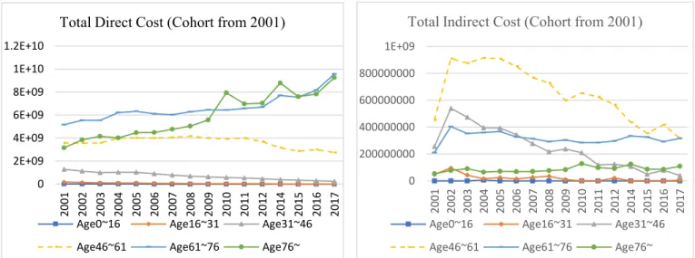
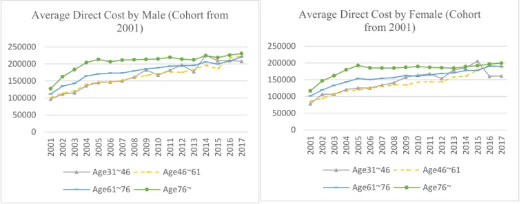
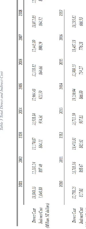
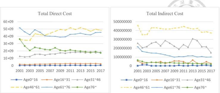
(27) 5.1.2. 2001 Cohort Follow-up The direct cost for elder patients is increasing. The age group of 61~76 is increased for 4 billion dollars and those above age 76 increase 6 billion. The indirect cost is decreasing from 2 billion to 874 million NT dollars for 16 years overall and each age group is decreasing. The average direct cost increases for patients above 31 years old both in male and female, and the older is the group, the higher is the cost. The drug expenses are increasing for the age above 61, otherwise, they are stationary over time. Since this is the follow up for the cohort, this indicates that the longer is the duration is the disease has affected the elder patients more than the younger ones. Total Indirect Cost (Cohort from 2001). Total Direct Cost (Cohort from 2001) 1.2E+10. 1E+09. 1E+10. 800000000. 8E+09. 600000000. 6E+09. 400000000. 4E+09. 200000000. 2E+09 2001 2002 2003 2004 2005 2006 2007 2008 2009 2010 2011 2012 2014 2015 2016 2017. 2001 2002 2003 2004 2005 2006 2007 2008 2009 2010 2011 2012 2014 2015 2016 2017. 0. 0 Age0~16. Age16~31. Age31~46. Age0~16. Age16~31. Age31~46. Age46~61. Age61~76. Age76~. Age46~61. Age61~76. Age76~. Figure 3 Total direct cost (cohort from 2001). Figure 4 Total indirect cost (cohort from 2001). 18.

(28) Average Direct Cost by Female (Cohort from 2001). Average Direct Cost by Male (Cohort from 2001) 250000. 200000. 200000. 150000. 150000. 100000. 100000. 50000. 50000. 0. 0 2001 2002 2003 2004 2005 2006 2007 2008 2009 2010 2011 2012 2013 2014 2015 2016 2017. 2001 2002 2003 2004 2005 2006 2007 2008 2009 2010 2011 2012 2013 2014 2015 2016 2017. 250000. Age31~46. Age46~61. Age31~46. Age46~61. Age61~76. Age76~. Age61~76. Age76~. Figure 5 Average direct cost among male (cohort from 2001). Figure 6 Average direct cost among female (cohort from 2001). 5.1.3. New cases cross-sectional from 2001 to 2017 For those new cases, the total direct cost is stationary around 13 billion NT dollars, but the average direct cost for both male and female are slightly increasing for these years. The total indirect cost is decreasing in general and decreasing largely in the age group of 31~46. The highest proportion for the drug expense is the age group 46~61 with the highest incidence. No matter the follow- up cohort or the cross-sectional data, the drug expense increases over time.. 19.

(29) 20. Table 3 Total Direct and Indirect Cost.

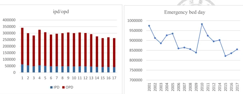
(30) Total Indirect Cost. Total Direct Cost 6E+09. 500000000. 5E+09. 400000000. 4E+09. 300000000. 3E+09 200000000. 2E+09. 100000000. 1E+09 0. 0 2001 2003 2005 2007 2009 2011 2013 2015 2017. 2001 2003 2005 2007 2009 2011 2013 2015 2017. Age0~16. Age16~31. Age31~46. Age0~16. Age16~31. Age31~46. Age46~61. Age61~76. Age76~. Age46~61. Age61~76. Age76~. Figure 7 Total indirect cost (cross-sectional). Figure 8 Total direct cost (cross-sectional). The ratio of IPD and OPD is stationary over time but decreasing overall. OPD is almost 6 times than IPD. The proportion of the number of emergency beds and the number of chronic beds is approximately 10:1 and the older the patients, the more emergency beds are needed. Emergency bed usage is decreasing over time.. Average Direct Cost by Male. Average Direct Cost by Female. 350000 300000 250000 200000 150000 100000 50000 0. 500000 400000 300000 200000. 2001 2002 2003 2004 2005 2006 2007 2008 2009 2010 2011 2012 2013 2014 2015 2016 2017. 100000 0 2001 2003 2005 2007 2009 2011 2013 2015 2017. Age31~46. Age46~61. Age31~46. Age46~61. Age61~76. Age76~. Age61~76. Age76~. Figure 9 Average direct cost among male (cross-sectional). Figure 10 Average direct cost among female (cross-sectional). 21.

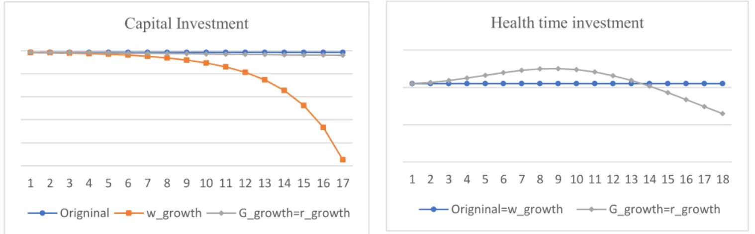
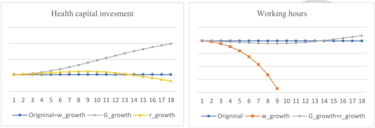
(31) Total Drug Expense. Total Drug Expense (Cohort from 2001) 800000000. 300000000. 700000000. 250000000. 600000000 200000000. 500000000. 150000000. 400000000 300000000. 100000000. 200000000. 2001 2002 2003 2004 2005 2006 2007 2008 2009 2010 2011 2012 2013 2014 2015 2016 2017. 2014. 2013. 2012. 2011. 2009. 2008. 2007. 2006. 2005. 2004. 0. 2003. 0 2002. 50000000 2001. 100000000. Age0~16. Age16~31. Age31~46. Age0~16. Age16~31. Age31~46. Age46~61. Age61~76. Age76~. Age46~61. Age61~76. Age76~. Figure 12 Total drug expense (cohort from 2001). Figure 11 Total drug expense (cross-sectional). 5.1.4. The Result of the Simulation In the simulation, the sustainable growth of wages, the interest rate for physical investment, and the yield of health investment are considered to observe the change in consumption, leisure time, capital investment, health time investment, health capital investment, and working hours. As the wage sustainably grows, the consumption in each period grows exponentially; the capital investment and working hours decrease exponentially. As the interest rate of physical investment increases sustainably, the consumption, leisure time spent, capital investment in each period decreases; Health capital investment and health time investment increase in the short run but decrease eventually. The working hours decrease in the short run but increases eventually. As the marginal product of health investment increases sustainably, consumption, capital, and leisure time decreases. Health time investment increases in the short run but decreases eventually. Health capital investment increases sustainably. The working hours decrease in the 22.

(32) short run but increase in the long run.. Consumption. Leisure time. 1 2 3 4 5 6 7 8 9 10 11 12 13 14 15 16 17 18 Origninal. 1 2 3 4 5 6 7 8 9 10 11 12 13 14 15 16 17 18. w_growth. r_growth=G_growth. Origninal=w_growth. Figure 14 Change in consumption. Figure 13 Change in leisure time. G_growth=r_growth. Capital Investment. Health time investment. 1 2 3 4 5 6 7 8 9 10 11 12 13 14 15 16 17. 1 2 3 4 5 6 7 8 9 10 11 12 13 14 15 16 17 18. Origninal. w_growth. Origninal=w_growth. G_growth=r_growth. G_growth=r_growth. Figure 16 Change in health time investment. Figure 15 Change in capital investment. 23.

(33) Health capital invesment. Working hours. 1 2 3 4 5 6 7 8 9 10 11 12 13 14 15 16 17 18. 1 2 3 4 5 6 7 8 9 10 11 12 13 14 15 16 17 18. Origninal=w_growth. G_growth. r_growth. Origninal. w_growth. G_growth=r_growth. Figure 17 Change in working hours. Figure 18 Change in health capital investment. 5.1.5. The Result of the Regression Model The result of the regression is presented in the table below. All of the coefficients except log (GDP) and log (DALY) are significant. The sign follows intuition except for education and labor. Education reflects that the enrollment rate of the college is not a good instrument variable. The opposite sign in labor may due to only the good quality that would affect economic growth. The coefficient of DALY was not significant. Even if I ignore the significance, the estimate is low. One percentage increasing of DALY only contributes to 0.066 percentage of decreasing GDP. The adjusted R-squared is 0.823 which is acceptable compare to the research conducted by Finlay, the adjusted R-squared is 0.82 which is similar to the result shown in the table below (Finlay, 2007).. 24.

(34) Table 4 The coefficients of the regression model. 6. Discussion The trend of the direct and indirect cost. The result of direct costs is consistent with the report from the Ministry of Health and Welfare. Yet, the expansion of drug expenses does not seem to slow down as a report from the Ministry of Health and Welfare. The indirect cost is decreasing in the follow-up cohort. This may due to mortality cost shares a high proportion of indirect cost; however, the potential loss from sick leave becomes lower as time passes. For the cross-sectional data, the indirect cost is mostly stationary. Since the patients in their 45~61 contribute the highest direct and indirect cost, the policymakers should find a way to control or delay the incidences. Vulnerable groups. The age of 41 to 76 contribute the most hypertensive patients. Also, the male is more likely to get hypertensive diseases, but the average cost does not show differences in both sexes. 25.

(35) Considering the whole population, the incidence rate is decreasing, especially in the age above 76. It’s largely decreasing over time. The trend of drug expense and comparison to other disease and countries. The drug expenses are increasing and especially for the elder. The drug expenses increase both in the follow-up cohort and the cross-sectional data. From the study of Chen, the price of foreign new brand name drugs is increasing, and the generic drug is decreasing from 1997 to 2004. From their research finding, the usage of the foreign new brand name drug is increasing while the usage of the generic drug is decreasing (陳美美, 林眉均, & 吳培滋, 2007). This leads to the expansion of the drug expense for hypertensive diseases. Also, some of the researches argue that there is a duplicate medicine problem for hypertension patients. As hypertension often comes with hyperglycemia and hyperlipidemia, duplicate medicine is easy to happen when the doctor prescribes the chronic prescription. Yet, with the NHI PharmaCloud program operated in 2014, the situation of duplicate medicine has been improved. The other possible reason is that the longer the duration of hypertension, the more and the higher dose of medicine is used for effective control of hypertension. The comparison to other research. The prevalence of hypertension according to the statistics from the Ministry of Health and Welfare, the age 50-59 is 34.8% and 60-69 is 54.5% (Ministry of Health and Welfare, 2007). From the results show above, the incidence is stationary over time. The prevalence proportion should be stationary as well. Compare to other countries, U.S. has about 53 percent of people in their age 50~65 get the hypertensive disease, and the U.K. has about 45 percent. People above 65, the prevalent proportion would be 51 and 42 percent. Taiwan’s situation seems to be better. 26.

(36) The coefficient of DALY is not significant, and the labor size and education have the opposite sign. The reason might be the college enrollment rate cannot reflect the progress of education and there might be too many confounders affect the labor market. Comparing to the literature review by Finlay, the result should be significant. The possible reason is that Finlay believes health may affect the model in two ways. One is through mortality. This would affect the size of the labor market. The other would be education. He believes health would affect the effectiveness of education. In this study, the disease burden includes the potential productivity loss that would make the effect vaguer. Another similar study is conducted to capture the effect of HIV by using the human capital methods cross countries. Although the results are not significant, the authors still consider there is some effect on HIV. The world average economic impact would be 0.05, which is similar to the results I get.. 7. Limitation One of the limitations of the study is the population of the whole hypertensive patients is unknown. I can only abstract the new cases from 2001 to 2017 and follow-up the 2001 cohort. Yet, some patients may not go to a clinic or hospital to take blood pressure due to mild syndrome, the medication allergic or the medication is futile. Also, the medical expenses should be calculated as unscheduled fees rather than NT dollars in the NHI system in Taiwan. It would be more precise if the study uses the chain method to discount the dollar in different years for comparison; however, I believe this would just be minor bias which would not affect the trend of the expenditure and the conclusion I made. Since the patients were included in our analysis if they have any of the primary or secondary diagnosis with hypertension, the economic impact may be under- or overestimate the indirect cost because some patients’ cost might mainly result 27.

(37) from other disease or causes. Also, there are other risk factors or confounder I might fail to consider. In this study, many coefficients are adopter from studies in other country which might leadl to biased estimation in this study. Most of the previous studies used survey data for cost estimation, which is lacking in Taiwan. Another limitation is that I calculated the economic cost assuming patients would be healthy if they were free from hypertension; however, competitive risk models consider patients who are free from specific disease may have the probability to get other diseases. Finally, in the simulation model, I tried to find the coefficient of the health time investing then I can take them back to the growth model; however, as the adaptive Grossman model is hard to estimate, I can only construct the dynamic simulation. Further analysis is encouraged to do in the future.. 8. Conclusion The economic impact of hypertension is large even if the effect on economic growth is not statistically significant. The direct cost including health expenditure is high. With the duration of hypertension getting longer, the expenditure is going to become greater. The drug expenses are especially huge and expand over time. The reason might be using more new brand name drugs and the higher dose or polypharmacy problems. Most of the patients come to the hospital for outpatient visits rather than inpatient visits. The mortality is decreasing especially for those aged above 61 years old. This is a good sign since the incidence proportion is high in the elderly people. To construct the growth model, this study considers the representative individual maximizing her infinite horizon utility. The results show after increasing physical capital, the health capital investment should increase to maximize their utility and boost economic growth. While increasing the incentive of health capital, the return of health capital or the marginal 28.

(38) product of health investment should be higher. By using the human capital method to estimate the economic cost for hypertension disease, the results show that the logarithm of DALY is not significant. To sum up, this study shows the heavy burden of hypertension, especially its drug expenses. Even the DALY in the growth model is not significant, DALY for the top ten diseases can be combined to be a health indicator. Further studies could construct an advanced and robust model for the relationship between health and economic growth.. 29.

(39) Reference Abegunde, D. O., Mathers, C. D., Adam, T., Ortegon, M., & Strong, K. (2007). The burden and costs of chronic diseases in low income and middle income countries. The Lancet, 19291938. Akobundu, E., Ju, J., & Mullins, L. B. (2006). Cost-of-Illness Studies-A review of Current Methods. Pharmacoeconomics. American Diabetes Association. (2008). Economic Costs of Diabetes in the U.S. in 2007. Alexandria: American Diabetes Association. Arno, P. S., Levine, C., & Memmott, M. M. (1999). The Economic Value Of Informal Caregiving. Health Affairs, 182-188. Bonita, R., Beaglehole, R., & Kjellstron, T. (2006). Basic Epidemiology Second Edition. Geneva: World Health Organization. Cervellati, M., & Sunde, U. (2005). Human Capital Formation, Life Expectancy, and the Process of Development. American Economic Association, 16533-1672. Chakraborty, S. (2004). Endogenous lifetime and Economic Growth. Journal of Economic Theory, 119-137. Chodick, G., Porath, A., Alapi, H., Sella, T., Flash, S., Wood, F., & Shalev, V. (2010). The Direct Medical Cost of Cardiovascular Disease, Hypertension, Diabetes, Cancer, Pregnancy and Female Infertility in a large HMO in Israel. Health Policy. CJ, M., & AD, L. (1997). Global Mortality, Disability, and the Contribution of Risk Factors: Global Burden of Disease Study. Lancet. Collins, J. J., Baase, C. M., Sharda, C. E., Ozminkowski, R. J., Nicholson, S., Billotti, G. M., . . . Berger, M. L. (2005). The Assessment of Chronic Health Conditions on Work Performance, Absence, and Total Economic Impact for Employers. Journal of Occupational and Environmental Medicine, 547-557. Finlay, J. (2007). The Role of Health in Economic Development. Program of the global demography of aging working paper. Goetzel, R. Z., Long, S. R., Ozminkowski, R. J., Hawkins, K., Wang, S., & Lynch, W. (2004). Health Absence, Disability, and Presenteeism Cost Estimates of Certain Physical and Mental Health Conditions Affecting U.S. Employers. Journal of Occupational and Environmental Medicine, 396-412. Grossman, M. (1972). On the Concept of Health Capital and the Demand for Health. Journal of Political Economy. Hu, Y.-N., Hu, G.-C., Hsu, C.-Y., Hsieh, S.-F., & Li, C.-C. (2012). Assessment of Individual Activities of Daily Living and its Association with Self-Rated Health in Elderly People of Taiwan. International Journal of Gerontology, 117-121. Institute for Health Metrics and Evaluation (IHME). (2010). Global Burden of Disease Study 2010 (GBD 2010) Disability Weights. Institute for Health Metrics and Evaluation (IHME). Johns, G. (2010). Presenteeism in the workplace: A review and research agenda. Journal of Organizational Behavior, 519-542. Kalemli-Ozcan, S., Ryder, H. E., & Weil, D. N. (2000). Mortality decline, human capital investment, and economic growth. Journal of Development Economics, 1-23. Kay, D., Pruss, A., & Corvalan, C. (2000). Methodology for assessment of Environmental burden of disease. Buffalo: August. 30.

(40) Liu, D.-P., Wang, T.-A., Huang, W.-T., Chang, L.-Y., Wang, E.-T., Cheng, S.-H., & Ming-Ching. (2015). Disease Burden of Enterovirus Infection in Taiwan: Implications for Vaccination policy. Vaccine. Ministry of Health and Welfare. (2007, July 26). Ministry of Health and Welfare. Retrieved from 2.1-09_20 歲以上民眾高血壓、高血糖、高膽固醇盛行率: https://dep.mohw.gov.tw/DOS/cp-1720-7332-113.html Muennig, P. (2007). Cost-Effectiveness Analysis in Health: A Practical Approach 2nd Edition. Jossey-Bass. National Health Insurance Administration. (2016). 2016-2017 National Helth Insurance Annual Report. Taipei: National Health Insurance Administration. Porta, M. (2014). A Dictionary of Epidemiology (5th ed.). Oxford: Oxford University Press. Ruiz-Hernandez, Tellez-Plaza, Dominguez-Lucas, Pichler, Martin-Escudero, MartinezGarcia, . . . Redon. (2018). Population Attributable Risk for Cardiovascular Disease Associated With Hypertension. Results from the Hortega Follow-up study. Journal of Hypertension, e27. Solow, R. M. (1956). A Contribution to the Theory of Economic Growth. Quarterly Journal of Economics. The Reporter. (2020, March 9). The Reporter. Retrieved from 病床邊的照護危機: https://www.twreporter.org/topics/nursing-aide-crisis-of-taking-care Weil, D. N. (2009). Economic Growth Second edition. Boston: Pearson. World Health Organization. (2019, March 7). World Health Organization. Retrieved from Metrics: Disability-Adjusted Life Year (DALY): https://www.who.int/healthinfo/global_burden_disease/metrics_daly/en/ World Health Organization. (2020, March 8). Disease burden and mortality estimates. Retrieved from WHO Web site: https://www.who.int/healthinfo/global_burden_disease/estimates/en/index1.html World Health Organization. (2020, March 8). Hypertension. Retrieved from WHO Web site: https://www.who.int/health-topics/hypertension/ 勞動部. (2010). 國民長期照護需求調查. 勞動部. Retrieved from 最新消息. 張國維. (2011). 誰需要長期照顧？慢性疾病擴張的討論. 社區發展季刊, 426-444. 衛生福利部健康保險署. (2010, February 9). 衛生福利部健康保險署. Retrieved from 健保公布 98 年藥費前十名藥品，三高用藥佔八成: https://www.nhi.gov.tw/News_Content.aspx?n=FC05EB85BD57C709&sms=587F1A3D 9A03E2AD&s=9129ECBFC31F42E2 陳美美, 林眉均, & 吳培滋. (2007). 以藥物經濟學觀點探討我國高血壓病患用藥之合理性. 台北: 衛生福利部.. 31.

(41) Appendix A. The Lagrange Methods for the Simulation The Lagrange function is noted as follow: L = ∑ 𝛽 𝑡−1 𝑢(𝑐𝑡 , 𝑡𝑙𝑡 ) + 𝜆𝑡 ∑ 𝛽 𝑡−1 (𝑎𝑡 + (1 − 𝑡𝑙 − 𝑡ℎ )𝑤𝑡 + (1 + 𝑟𝑡−1 )𝐼𝑘𝑡−1 + (1 + 𝑟ℎ𝑡−1 )(𝑡ℎ𝑡 𝐺ℎ𝑡 + 𝐸𝑥𝑝ℎ ) − 𝑐𝑡 − 𝐼𝑘𝑡 − (𝑡ℎ𝑡 𝐺ℎ𝑡 + 𝐸𝑥𝑝ℎ )) First-order condition: 𝑢𝑐 (𝑐𝑡 , 𝑡𝑙 ) = 𝜆𝑡 𝜆𝑡 is the marginal utility of consumption. 𝑢𝑡𝑙 (𝑐𝑡 , 𝑡𝑙 ) = 𝜆𝑡 𝑤𝑡. The marginal utility of leisure is equal to the opportunity cost of work. 𝜆𝑡 = 𝛽𝜆𝑡+1 (1 + 𝑟𝑡 ) The marginal utility of consumption must equal to the utility discounted in the future. 𝑟ℎ𝑡−1 Ght = 𝜆𝑡 𝑤𝑡 The opportunity cost of working equal to the opportunity cost of investing health capital. 𝑟ℎ𝑡 = 𝑟 − πt−1 + 𝛿𝑡 The relationship between the return from investing in health and physical capital; πt is the percentage rate of change in marginal cost invest in health. 𝛿𝑡 stands for the depreciation for the physical capital. Consider the utility function as 𝑢(𝑐𝑡 , 𝑙𝑡 ) = 𝛼ln𝑐𝑡 + (1 − 𝛼)𝑙𝑡 , 𝛼 ∈ (0,1);. 𝜕𝐿 α =0⇒c= 𝜕𝑐 𝜆 𝜕𝐿 1−𝛼 = 0 ⇒ tl = 𝜕𝑡𝑙 𝜆𝑤 𝜕𝐿 =0⇒r=ρ 𝜕𝐼𝑘 𝜕𝐿 rh 𝐺 𝐺(𝑟 − 𝜋 + 𝛿) =0⇒λ= = 𝜕𝑡ℎ 𝑤 𝑤. Take these equations back into the budget constraint then done.. 32.

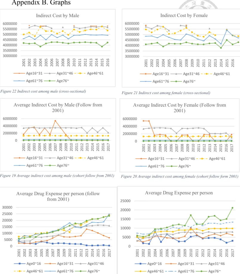
(42) Appendix B. Graphs Indirect Cost by Female. Indirect Cost by Male 6000000 5500000 5000000 4500000 4000000 3500000 3000000. Age16~31. Age31~46. Age61~76. Age76~. 2001 2002 2003 2004 2005 2006 2007 2008 2009 2010 2011 2012 2013 2014 2015 2016. 2001 2002 2003 2004 2005 2006 2007 2008 2009 2010 2011 2012 2013 2014 2015 2016. 6000000 5500000 5000000 4500000 4000000 3500000 3000000. Age46~61. Figure 22 Indirect cost among male (cross-sectional). 4000000. 4000000. 2000000. 2000000. 0. 0. Age76~. Age76~. 2001 2002 2003 2004 2005 2006 2007 2008 2009 2010 2011 2012 2013 2014 2015 2016 2017. 2001 2002 2003 2004 2005 2006 2007 2008 2009 2010 2011 2012 2013 2014 2015 2016 2017. 6000000. Age61~76. Age61~76. Age46~61. Average Indirect Cost by Female (Follow from 2001). 6000000. Age31~46. Age31~46. Figure 21 Indirect cost among female (cross-sectional). Average Indirect Cost by Male (Follow from 2001). Age16~31. Age16~31. Age46~61. Age16~31. Age31~46. Age61~76. Age76~. Age46~61. Figure 19 Average indirect cost among male (cohort follow from 2001). Figure 20 Average indirect cost among female (cohort follow form 2001). Average Drug Expense per person (follow from 2001). Average Drug Expense per person 25000. 30000. 20000. 25000 20000. 15000. 15000. 10000. 10000. 5000. 5000 0. 2001 2002 2003 2004 2005 2006 2007 2008 2009 2010 2011 2012 2013 2014 2015 2016 2017. 2001 2002 2003 2004 2005 2006 2007 2008 2009 2010 2011 2012 2013 2014 2015 2016 2017. 0. Age0~16. Age16~31. Age31~46. Age0~16. Age16~31. Age31~46. Age46~61. Age61~76. Age76~. Age46~61. Age61~76. Age76~. Figure 24 Average drug expense per person (cohort follow from 2001). 33. Figure 23 Average drug expense per person (cross-sectional).

(43) ipd/opd. Emergency bed day. 400000. 1000000. 350000. 950000. 300000 250000. 900000. 200000. 850000. 150000 100000. 800000. 50000. 750000. 0. IPD. 700000 2001 2002 2003 2004 2005 2006 2007 2008 2009 2010 2011 2012 2014 2015 2016 2017. 1 2 3 4 5 6 7 8 9 10 11 12 13 14 15 16 17 OPD. Figure 26 Emergency bed day. Figure 25 The ratio of IPD over OPD. 34.

(44) Appendix C. NHID Application Form. 35.

(45) 36.

(46) 37.

(47) 38.

(48) 39.

(49) 40.

(50) 41.

(51) 42.

(52) 43.

(53) 44.

(54)