於具有攻擊偵測機制之過程控制系統上論潛伏攻擊之影響

(1)

國立交通大學

電控工程研究所

碩士論文

於具有攻擊偵測機制之過程控制系統上論潛伏攻擊之影響

On Study of Stealthy Attacks in a Process Control System with

Model-based Anomaly Detection Protection

研究生：黃啟彥

Student: Chi-Yen Huang

指導教授：黃育綸博士

Advisor: Dr. Yu-Lun Huang

中華民國九十九年一月

January, 2010

(2)

於具有攻擊偵測機制之過程控制系統上論潛伏攻擊之影響

On Study of Stealthy Attacks in a Process Control System with Model-based

Anomaly Detection Protection

研究生：黃啟彥 Student: Chi-Yen Huang

指導教授：黃育綸博士 Advisor: Dr. Yu-Lun Huang

國立交通大學電控工程研究所

碩士論文

A Thesis

Submitted to Institute of Electrical Control Engineering College of Electrical Engineering

National Chiao Tung University in partial Fulfill of the Requirements

for the Degree of Master

in

Institute of Electrical Control Engineering

January, 2010

Hsinchu, Taiwan, Republic of China

(3)

於具有攻擊偵測機制之過程控制系統上論

潛伏攻擊之影響

學生：黃啟彥

指導教授：黃育綸博士

國立交通大學電控工程研究所碩士班

摘

要

過程控制系統(PCS)具有穩定系統運作的能力，常被廣泛應用於現今的基礎建設及大型工廠中。由於這類系統的任何毀損都可能造成極重大的災難，並奪走數千條人命，因此2008年即有研究學者針對Tennessee-Eastman過程控制系統(TE-PCS)提出一套以模型為基礎的攻擊偵測模組(mADM)，確保TE-PCS能維持在穩定的工作範圍內。 mADM利用真實訊號與內部模擬訊號的累計差值，來推斷系統的感測器是否遭人破壞，而對系統進行不利之攻擊。為保證PCS受到mADM的良好保護，在本篇論文中，我們以內賊的角度，對系統進行潛伏攻擊，以評估mADM之強健性。所謂內賊即為可能(1)熟知mADM的運作與參數或(2)擁有更改mADM參數權力之人；透過潛伏攻擊，可以在不被 mADM偵測的情況下，使系統不當運作，而造成營運成本上升或工廠機具毀損。在分析 mADM的設計後，我們依據累計差值的曲線變化，設計三種訊號曲線（凸面、斜線和凹面），以組成各種不同類型的潛伏攻擊，並進一步地攻擊以mADM保護之PCS。以 TE-PCS為例，我們設計一系列的實驗，找出最有效的攻擊目標(感測器)和其相對應之攻擊方法。實驗結果證明當mADM參數落於安全範圍值時，潛伏攻擊無法造成系統崩解。但是，如果內賊擁有更改mADM參數的權力，則系統必須嚴加控管mADM參數的設定，否則過高的參數值會使系統遭受攻擊而損毀，過低的值則會使系統頻繁地發出錯誤警示，而增加營運成本。最後，我們演示三個例子，說明在不同的收支比下，潛伏攻擊

(4)

(5)

On Study of Stealthy Attacks in a Process Control System

with Model-based Anomaly Detection Protection

Student: Chi-Yen Huang

Advisor: Dr. Yu-Lun Huang

Institute of Electrical Control Engineering

National Chiao Tung University

Abstract

Process control systems (PCS) are widely used in modern infrastructures and industrial plants for stabilizing safety-critical processes. Any disruption in such systems may cause serious human injuries and environmental disasters. In 2008, Lin et al. proposed a model-based anomaly detection module (abbreviated to mADM) to assure the security and stability of a well-studied Tennessee-Eastman process control system (TE-PCS). By taking advantages of cumulating the differences between real and simulated signals, mADM was able to detect an attack that com-promises one or more sensors to crash the system. To evaluate the robustness of mADM, we study the stealthy attacks launched by an insider who may (1) know the detection and response strategies of mADM or (2) adjust the parameters of mADM so that these stealthy attacks may successfully attack the system without being detected by mADM. After analyzing mADM, we prove that a general stealthy attack signal can be represented by three types of curves, convex curve (cv), slope (sl), and concave curve (cc), depending on the cumulative differences of sig-nals. By conducting a series of experiments on TE-PCS, we can identify the weakest sensor and the most effective way to stealthily attack this sensor. We also show that, if an insider cannot adjust the parameter settings and the parameters are well configured, he may not be able to crash the system. In the case that the insider obtains the permission to adjust the parameter settings,

(6)

mADM should self-check whether the settings fall within valid ranges. Over-the-threshold set-tings may lead to a crash without being detected while under-the-threshold values may result in frequent false alarms and increase the operating costs. In the end, we also demonstrate three case studies to discuss that stealthy attacks may decrease the profits from 0.06% to 41%, depending on the ratio of costs and sales prices.

(7)

謝誌

猶如每位得獎者感言所述：「謝謝父母、家人給我的鼓勵與支持……」成就一件事物要謝天、謝地、謝東、謝西、謝南、謝北，要感謝的除了人，還有天地萬物，怎麼也謝不完。以下將以寥寥數字，重點感謝身邊的人事物，其未於文中提及者，便以陳之藩先生最常被引用的名句：「因為需要感謝的人太多了，就感謝天罷。」一併感謝之。能夠完成此篇論文首先感謝余之業師黃育綸博士，教授為我大學時代之導師，在學業上即有相當的提點，一路到研究所，更是教會我如何發現問題、研究問題、解決問題。也感謝老師參加iCAST (The International Collaboration for Advancing Security Technology)計劃，提供我赴美國加州柏克萊分校機會，接受Doug Tygar教授、Alvaro Cardenas、Saurabh Amin博士的提攜。另外感謝於柏克萊認識的朋友(特別是黃氏同宗的湘瑀大姊)，有你們的相互扶持，才得以讓我這隻身異鄉客有所依靠。接下來此段落我們將討論實驗室室友對一研究生之影響。曾勁源學長:一表人才的大師兄，對人親切和藹，帶我去聯誼和我打桌球。蔡欣宜學姊:鄰座大師姊是遇到問題時的最佳求救對象，曾透過電扇聽我告解。黃詠文學長:從Sopca星球來，人人都欠他幾億，碰到技術上的困難，找他必解。鍾興龍學長:客家阿龍教我客語，帶我去爬仙山。張立穎學長:進lab時正逢學長準備畢業，讓我了解到報告的形式。陸培華學長:相處時間不長，但也是我入門時期的重要影響者。洪精佑學長:生動活潑的鵰兄，是我的菜。王鈺婷學姊:常常奮戰到天亮的summation，讓我知道什麼才叫做研究。甄元彬學長:有阿彬陪我遊山玩水，說衝就衝，實在難能可貴。許正道學長:道道正經的表面下，暗藏不少爆點。張宗堯學長:小狼常提供我諮商，是心靈上的好夥伴。陳柏廷學長:龜槍學長小叮噹，為一可敬的牌咖。林宗勳學長:基於帥勳的東西，我才能順利走到今天。夏拉喬學姊:shylu親自下廚，引我品嚐新奇的印度口味。吳思穎同學:思思姊也是牌場上的

(8)

女中豪傑。王雅萱同學:多謝鄉鄉姊在美國的照應，莫名的笑點，引人苦笑。彭博群同學:有讀書強迫症的澎哥，沉著穩重的個性收斂了我的性格。黃晉澤同學:從大學到研究所變了很多的睪哥，不失為一好玩伴。吳嘉稘學弟:愛嗆學長姊的稘稘，謝謝你沒冒犯我。許鴻生學弟:超像Judo的Juju，取代wiper精實的臂膀。鄭偉強學弟:比我還好動的強強，展現了許多生活小智慧。黃錦銘學弟:有敏敏加入RTES，大家的啟笑聲分貝更是一天大過一天！黃奕奇學弟:先感謝你還沒寄來的賀年卡。葉書宏學弟:雖然酥酥還沒進來，相信你能挑起實驗室大樑的。賴鈺婷學妹:謝謝嗨嗨上回帶來的伴手禮。實驗室有以上所有人同進退地陪伴，或多或少影響著每日的生活，讓研究所生涯充滿歡笑，少了妳/你們，生活一定沒那麼多姿采。除此之外還有97級同學們、電控學長姊、學弟妹、電機學弟妹，認識妳/你們使我竊得認識王之名。最後還要感謝交大電機系壘，有你們，使我的休閒時光更精彩。在此以詩一首警惕自己莫忘吾師。 Figure 1: Key=717613121192

(9)

List of Figures

2.1 PCS . . . 5

2.2 Simpliﬁed TE-PCS with four control loops . . . 7

2.3 Threats to PCSs . . . 8

2.4 mADM . . . 8

2.5 General S(k) without attacks . . . 10

2.6 Diﬀerence between plant and linear internal model . . . 11

3.1 S(k) curve under stealthy attack . . . 14

3.2 S(k) of a cv attack . . . 15

3.3 S(k) of a sl attack . . . 16

3.4 S(k) of a cc attack . . . 17

4.1 Pressure of the reactor under 3 types of stealthy attacks on S1starts from 0 hr and ends at 1_{∼ 40 hrs . . . 24}

4.4 Pressure of two sensors attacked . . . 28

4.5 Pressure of two sensors attacked with diﬀerent b . . . 29

4.6 Pressure of the reactor under cv on S3starts from 0 hr and ends at 1∼ 40 hrs and cc on S2starts from 0 hr and ends at 1∼ 40 hrs with 0.5τLin . . . . 30

4.7 Pressure of the reactor under cv on S3starts from 0 hr and ends at 1∼ 40 hrs and cc on S2starts from 0 hr and ends at 1∼ 40 hrs with 1.5τLin . . . . 30

(12)

5.2 Function of pressure . . . 35

5.3 high proﬁt . . . 36

5.4 medium proﬁt . . . 37

(13)

List of Tables

4.1 Exp#1: Eﬀect of Diﬀerent Attacks . . . 20

4.2 Exp#2: Eﬀect of Attacking Two Sensors . . . 21

4.3 Exp#3: Eﬀect of Diﬀerent Attack Timing . . . 21

4.4 Exp#4: Eﬀect of Diﬀerent b . . . 22

4.5 Exp#5: Eﬀect of Diﬀerent τ . . . 23

(14)

Chapter 1 Introduction

1.1 Motivation

Process control systems are capable of monitoring, computing, and managing to stabilize safety-critical processes [1] in infrastructures [2] and industrial plants. Process control systems are composed of a set of networked devices, such as sensors, actuators, controllers and commu-nication devices [3], [4]. Recent researches have pointed out new vulnerabilities and threats in the process control systems [5], [6], [7], [8]. While most of the researches [9] and [10] utilize IT technologies to solve the cyber-security issues of process control systems, [5] discusses the differences between traditional IT security and process control system security.

Since process control systems are using in infrastructures and industrial plants, any disrup-tion of these systems can cause serious damage to human lives. Fault diagnosis and fault-tolerant control enables systems to operate properly when a component failure occurs. The system iso-lates the detected failed component and reconfigures the control loop to ensure the proper op-eration. Sensors measurements compromised attacks are different from sensor failures. The attack signal is located in the range of normal sensed values so fault diagnosis and fault-tolerant control cannot detect the attack.

In order to protect the process control systems from critical sensor measurements compro-mised attacks, a threat assessment methodology is developed and attacks detection and response

(15)

mechanisms are designed by Lin et al. [11]. Lin et al. proposes a model-based anomaly detec-tion module (mADM) to protect the process control systems from compromised sensor attacks. By using mADM with the trained parameters, PCSs can avoid being attacked by DoS or in-tegrity attacks. mADM sees sensor failures as attacks. When a sensor fails, mADM replaces the sensed signal with the simulated signal and send an alert to administrator.

In this thesis, we consider a more elaborated attack, stealthy attack, other than DoS or in-tegrity attacks. Following the study of [11] experimenting and simulating on a realistic chemical reactor plant [12], [13], we play as an insider conducting a series of stealthy attacks. We evalu-ate the robustness of the defense mechanism by two cases, (1) an insider knows all the parameters of the mADM or (2) an insider obtains the permission to adjust the parameter settings.

1.2 Contributions

In this thesis, we design a general stealthy attack signal and propose three kinds of different stealthy attack models. By launching these stealthy attacks, we intend to analyze the pressure variation of the reactor to see the effectiveness of mADM protecting the system. Moreover, a way to evaluate the cost of the system is proposed to understand the changing before and after launching stealthy attacks. We analyze the abilities of stealthy attacks causing explosion to the reactor and increasing the cost of the system to evaluate the robustness of mADM.

1.3 Synopsis

This thesis is organized as follow. In Chapter 2, a general PCS, the TE-PCS, and the mADM are introduced in detail. Chapter 3 describes the stealthy attack models. Chapter 4 shows the experiments results after launching different kinds of stealthy attacks. In Chapter 5, effect of

(16)

using different parameters of the mADM are analyzed. In addition, we evaluate the effect of stealthy attacks by seeing PPI variations indicating the system cost and by counting the earnings of products with different profits. Finally Chapter 6 concludes.

(17)

Chapter 2 Background

In this section, we will describe process control systems (PCSs), a well-studied process control system, Tennessee-Eastman process control system (TE-PCS) model [12], Ricker's proportional-integral (PI) control loops for the simplified TE process [13] and the mADM which is proposed by Lin et al. [11].

2.1 Process Control System (PCS)

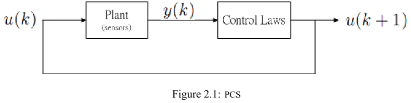
PCSs are widely used in our daily life to monitor and control processes such as transmission, distribution of utility services, and manufacturing factories. Take modern water distribution for example. Waterworks receive monitored data of the tank levels, the pressure of storage tanks, pH, turbidity, and chlorine residual in the tanks from remote sensors. Depending on these data, waterworks control the pumps [14] or the gates [15] and addition of chemicals to the water [16], [17], [18]. The factory or the plant here, works under the instruction of control commands u(k) at time k. And there are sensors monitoring the plant's statuses. Getting the sensed values y(k) at time k from the sensors, the controllers give the control commands u(k + 1) for the next time slot k + 1 depending on the control laws. The whole process can be shown as Fig. 2.1.

(18)

Figure 2.1: PCS

2.2 TE-PCS

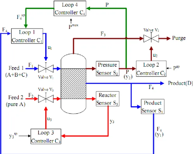
In this subsection, we are going to introduce the TE-PCS that we use as our experimental environment in detail. The original complex TE-PCS model [12] is simplified by Ricker [13]. Originally there are 41 measured output variables and 12 manipulated variables but are reduced to 10 and 4. Ricker also proposes the multi-loop PI control laws to control the simplified TE process at the steady state. The chemical process comprises two non-condensable reactants A and C, an inert B, and non-volatile liquid product D.

A + C −→ DB

Three of the ten measured output variables (denoted by yi, i = 1, 2, 3) are sensed by three sensors

and are used in the multi-loop PI control laws to control the four manipulated variables. The objectives of the control laws are to regulate the production rate of product D at set-point F₄sp (kmol h−1), to keep pressure of the reactor P under the crash limit, 3000kP a, and to maintain the ratio of ingredient A in reactor at set-point y₃sp (kmol h−1). Base on the objectives, Fig. 2.2 shows how Ricker's control loops work.

• Control loop 1:

Control loop 1 includes product sensor S1, loop 1 controller C1, and feed 1 valve V1. The

production rate F4 = y1 is sensed by S1 and is sent to C1. After computing the control

(19)

ingredients F1 bases on F

sp

4 to regulate F4.

Control loop 2 contains pressure sensor S2, loop 2 controller C2, and purge valve V2. The

pressure of the reactor P = y2 is sensed by S2 and is sent to C2. After computing the

control signal u2, C2tunes V2 opening rate according to u2. C2 controls P by letting less

vapor in reactor out when P is over low comparing to Psp_{, and vice versa.}

Control loop 3 involves reactor sensor S3, loop 3 controller C3, and feed 2 valve V3. The

fraction of ingredient A in reactor y3 is sensed by S3 and is sent to C3. After computing

the control signal u3, C3 adjusts V3 opening rate according to u3. C3 maintains y3 at y

sp

3

by adjusting V3.

Control loop 4 is composed of pressure sensor S2, loop 4 controller C4, C1and V1. When

P was over high (Pmax _{= 2900kP a), u}

2has the chance to saturate. Therefore C4changes

set-point F₄sp to shrink u1and further lower P .

These control loops helps the system to operate at the steady-state where the production rate

F4 = y1 is 100kmol, the pressure P is 2700kP a, and the fraction of ingredient A in reactor y3

(20)

(21)

2.3 mADM

In [11], Lin et al. assess the new vulnerabilities and threats to PCSs (Fig. 2.3). He aims

Figure 2.3: Threats to PCSs

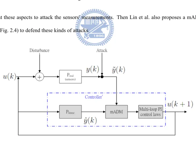
at these aspects to attack the sensors' measurements. Then Lin et al. also proposes a mADM (Fig. 2.4) to defend these kinds of attacks.

Figure 2.4: mADM

Lin et al. take simplified TE-PCS [13] to do his simulation. The main attacking goal that Lin et al. want to achieve is to drive the pressure of the TE reactor over 3000kPa (unsafe state).

(22)

It can be realized by launching attacks proposed in [19], [20], [21]. Lin et al. also add a Gaussian disturbance with variance 0.2 and zero mean to the control inputs u(k) to make the system real-like. For defending these attacks, a mADM is proposed. In order to detect attacks, the module uses the cumulative sum mechanism to cumulate the output differences between the TE-PCS model (˜y(k)) and the representative model (ˆy(k)) at time k. The representative model is

an internal linear model which satisfies the timing correctness in real time requirements. In each time slot k, the cumulative sum S(k) equals to the differences between ˜y(k) and ˆy(k) subtracted

by a tolerated difference b and adds to the previous cumulative sum S(k− 1) (Eq. (2.1)).

S(k) = S(k− 1) + |˜y(k) − ˆy(k)| − b, S(0) = 0 (2.1)

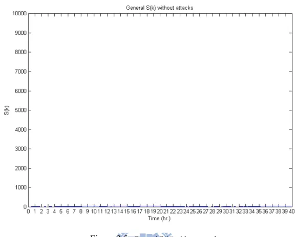
S(k) equals to zero when S(k) is smaller than zero. Generally, S(k) fluctuates around zero

because the mean of the added disturbance is zero Fig. 2.5. When S(k) is under the threshold

τ , the controller uses the outputs of the simplified TE-PCS model. Once the cumulative sum

exceeds τ , the mADM gives the outputs of the linear model to the controllers and sends out an alert to the administrator.

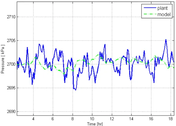
As shown in Fig. 2.6, b is the mean of the outputs difference between the simplified TE-PCS model under no attacks (the blue line) and the internal linear model (the green dotted line). τ is chosen by the tradeoff of false alarm rate and detection time. A mis-chosen b or τ affects the mADM seriously. If b is larger than it is supposed to be, the cumulative sum will never grow high enough to reach τ . In other words, the module will never have the chance to detect the attacks. On the contrary, if b is chosen smaller, the cumulative sum will cumulate because of the noise even when there is no attack. There will be false alarms all the time. A mis-chosen

τ has the same bad effect to the system. Larger τ prolongs the detection time, and hence the

module loses the prime time to discover an attack. The smaller τ may reduce the detection time. It is also easy to make the cumulative sum exceed τ and causes a false alarm. b and τ should

(23)

Figure 2.5:General S(k) without attacks

be carefully chosen before the module goes online, because these two parameters are the key points to make a robust mADM. Lin et al. set bLin = [0.0629, 1.7868, 0.0151] and τLin = [50

(24)

(25)

Chapter 3 Modeling Stealthy Attacks

We now consider an insider (1) who knows every parameter including: the output of internal linear model ˆy(k), b, and τ of the mADM or (2) the insider get the permission to modify b and τ .

The insider may carry stealthy attacks that can avoid being detected by the mADM. Fake sensed values locating between the minimum and the maximum value sensed by a normal sensor are given to the mADM by the insider as stealthy attack signals. From Eq. (2.1), we know the detection scheme cumulates the difference between modified sensed value ˜y(k) and the output

of internal linear model ˆy(k). For the convenience to manipulate S(k) under τ , we assume

the insider designs the attack signals as ˜y(k) = ˆy(k)− δ. By nullifying ˆy(k), the insider can

manipulate δ as any values to make sure that S(k) never exceeds τ .

We expand the causal equation S(k) = S(k− 1) + |˜y(k) − ˆy(k)| − b at time k = n to have a clearer sight in making sure that S(k) is always less than τ .

Theorem 1. The increment quantity of S(k) in period n is the summation of the output

differ-ences in period n between modified sensed value ˜y(k) and the internal linear model ˆy(k) from k = 1 to k = n, and minuses nb. S(n) = n ∑ k=1 |˜y(k) − ˆy(k)| − nb (3.1)

(26)

Proof. We shall prove the theorem by induction on n. assume S(0) = 0 let k = 0⇒ S(0) = 0 k = 1⇒ S(1) = 0 + |˜y(1) − ˆy(1)| − b .. . if k = n− 1 ⇒ S(n − 1) = n−1 ∑ k=1

|˜y(k) − ˆy(k)| − (n − 1)b holds

by induction

k = n⇒ S(n) = S(n − 1) + |˜y(n) − ˆy(n)| − b =

n

∑

k=1

|˜y(k) − ˆy(k)| − nb holds

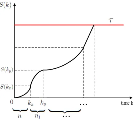
Let n = kx, from Theorem 1, attacker can drive S(k) from 0 to S(kx) in n slots. If

at-tacker wants to drive S(k) from S(kx) to S(ky) in next n1 = ky− kx slots, he can just simply

add∑ky

k=kx+1|˜y(k) − ˆy(k)| − n1b to S(kx). As in (Fig. 3.1), any attacks increase S(k). This

incremental curve is composed by convex curves, slopes, and concave curves if the curve is di-vided into several line segments. These three kinds of curves represent three kinds of attacking behaviors. Steeper slope of the curve implies stronger attack. Convex curve means the attack mitigates the strength when time passes by. Slope means the attack keeps same strength. As for the concave curve, the attack strength is enhanced with time. We model these three kinds of attacks as δ = βαn−k, where β is a positive number varies with α and n. α is a positive constant determines the bending degree. n = kx− ky is the attack duration and k is the time slot where

kx < k≤ ky (Fig. 3.1).

(27)

Figure 3.1: S(k) curve under stealthy attack

curves. Hence a general formula for the stealthy attack signal is shown below:

˜

y(k) = ˆy(k)− βαn−k (3.2) For simplicity, we assume the attack starts from kx = 0 and ends at ky = n. The cumulative sum

reaches the threshold τ at time k = n while the attack is ceased. Substituting ˜y(k) in Eq. (3.1)

by Eq. (3.2), we can get Eq. (3.3). By choosing a constant α, the inside attacker can find an appropriate β that satisfies S(n) ≤ τ. The attacker can generate the stealthy attack signal by solving the equation

S(n) =

n

∑

k=1

βαn−k − nb ≤ τ (3.3) Since α and n are chosen constants, from the formula of the first n term of geometric series with the common ratio̸= 1, β = τ +nb1−αn

1−α

can be solved.

According to the constant value of α, we categorize stealthy attacks into three types: convex

(28)

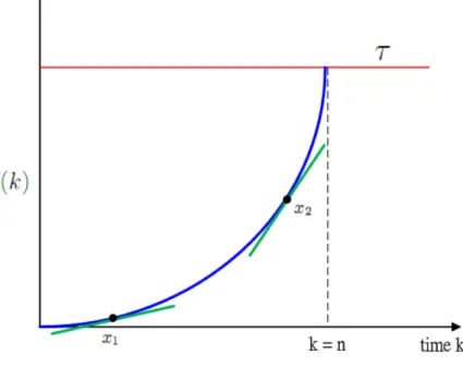
3.1 Convex Curve (cv) Attacks

In a convex curve attack, the attacker makes the maximum damage to the system in a short time period. By Eq. (3.2), this kind of attack signal can be generated by choosing α > 1. In Fig. 3.2, S(k) approaches τ very fast at the beginning of the attack but slow down when k is close to n and stop growing at k = n. Since slope x1 > x2, we know the strength of the attack

is strong at the beginning but diminishes at the rest of the attack duration. The strong variance at the beginning may cause high attention. Hence cv attack may not be so harmful.

Figure 3.2: S(k) of a cv attack

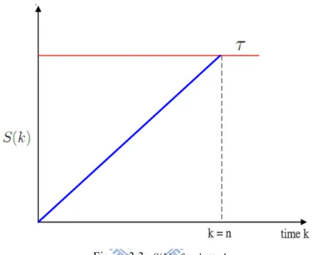
3.2 Slope (sl) Attacks

In a slope attack, the attacker keeps attack signal ˜y(k) a constant difference δ to ˆy(k) which

means selecting α = 1 in Eq. (3.2). So the equation

n−1

∑

k=0

(29)

is reduced to nβ− nb = τ. When β = b + τ/n, S(k) is a constant slope (Fig. 3.3) growing from attack starts and reaching τ at the end of the attack (k = n). There is no variance strength in this kind of attacks because the slope is always the same. sl attack always keeping the same pace is a moderate attack comparing to cv and cc attacks.

Figure 3.3:S(k) of a sl attack

3.3 Concave Curve (cc) Attacks

In a concave curve attack, the attacker chooses α < 1 in Eq. (3.2), which causes serious damage at the end of the attack instead of the beginning. S(k) is a contrast to cv. We can see in Fig. 3.4, S(k) starts slowly and ends severely to reach τ at time k = n. The slope of cc is always larger (x1 < x2) one time slot after another so we know that the strength keeps stronger

(30)

(31)

Chapter 4 Experiments

In this chapter, we run the three kinds of stealthy attacks mentioned above to test how much damage these attacks can cause to the explosion of the reactor. The experiments settings are as following:

4.1 Setup

In order to see how the stealthy attacks will affect the TE-PCS with the mADM proposed by Lin et al. , we use the following three components to simulate the experiments:

• TE-PCS model: The model written in .f file should be compiled into .mexw32 format by

Intel Visual FORTRAN compiler ver. 11. 0. The codes can be got by sending an e-mail to [email protected]

• PI control laws: The codes written in .M file running on MATLAB ver. 7. 8. 0. 347 can

be got by sending an e-mail to [email protected]

• mADM: The codes written in .M files running on MATLAB ver. 7. 8. 0. 347 can be got

(32)

4.2 Experiments

We design a formal format for stealthy attack which can be represented by 5 tuple as

{< A, S, Ts, Te, τsa>+}.

• A: the type of stealthy attack (cv, sl, or cc) • S: the victim sensor (S1, S2, or S3)

• Ts: the time that attack starts

• Te: the time that attack ends

• τsa: the value that Si(k) reaches

In addition,+_{indicates one or more sensors are attacked. In this section, we design experiments}

launching cv, sl, and cc attacks mentioned in the previous chapter. For an insider knowing the parameters of mADM, we conduct Exp#1 and Exp#2 to find the weakest sensor and the relative type of stealthy attack. In Exp#3 we launch the most effective attacks derived from the first two experiments on sensors with different starting time to find the most effective attack timing. For an insider getting the authority to configure the parameters of mADM, we conduct Exp#4 and Exp#5 to see the robustness of mADM with different bs and τ s.

4.2.1 Exp#1: Effect of Different Attacks

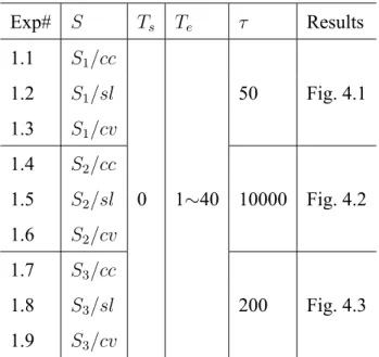
In the first experiment (Exp#1), we want to know what type of attack is more effective in driving the pressure up for each sensor. Thus we launching different attacks on different sensors in Exp#1. 1∼Exp#1. 9 (Table 4.1 ).

In Exp#1, b and τ are the best values recommended by Lin et al. , b = bLin = [0.0629,

(33)

Table 4.1: Exp#1: Effect of Different Attacks Exp# S Ts Te τ Results 1.1 S1/cc 1.2 S1/sl 50 Fig. 4.1 1.3 S1/cv 1.4 S2/cc 1.5 S2/sl 0 1∼40 10000 Fig. 4.2 1.6 S2/cv 1.7 S3/cc 1.8 S3/sl 200 Fig. 4.3 1.9 S3/cv S1, 0, 1∼40, 50>}, {< sl, S1, 0, 1∼40, 50>}, {< cv, S1, 0, 1∼40, 50>}, {< cc, S2, 0, 1∼40, 10000>}, {< sl, S2, 0, 1∼40, 10000>}, {< cv, S2, 0, 1∼40, 10000>}, {<cc, S3, 0, 1∼40,

200>}, {< sl, S3, 0, 1∼40, 200>}, and {< cv, S3, 0, 1∼40, 200>}. For Exp#1. 1∼Exp#1. 3

we start the attacks from Ts = 0 and end the attacks at Te = 1 to Te = 40. Driving the S(k) to

50, we stealthily attack S1by cv, sl, and cc attacks to see which types of attack is more effective

in driving up the reactor's pressure. Similarly, we attack S2 in Exp#1. 4∼Exp#1. 6 and S3 in

Exp#1. 7∼Exp#1. 9.

4.2.2 Exp#2: Effect of Attacking Two Sensors

In the second experiment (Exp#2), we consider the effect of attacking two sensors at a time when driving up the pressure of the reactor. Hence we design the attack as show in Table 4.2.

In Exp#2, b and τ are also the best values recommended by Lin et al. , b = bLinand τ = τLin.

The experiment can be represented as{< cv, S1, 0, 1∼40, 50>, < cc, S2, 0, 1∼40, 10000>},

(34)

Table 4.2: Exp#2: Effect of Attacking Two Sensors Exp# SI SII Ts Te τI τII Results 2.1 S1/cv S2/cc 0 1∼40 50 10000 Fig. 4.4a 2.2 S2/sl Fig. 4.4b 2.3 S3/cv S2/cc 200 Fig. 4.4c 2.4 S2/sl Fig. 4.4d

1∼40, 10000>}, and {< cv, S3, 0, 1∼40, 200>, < sl, S2, 0, 1∼40, 10000>}. Here we attack

S1 from Ts = 0 to Te = 1 ∼ 40 to drive the S(k) to 50. At the meanwhile, we also attack S2

from Ts = 0 to Te = 1 ∼ 40 to drive the S(k) to 10000. Similarly, we attack S2 and S3 at

a time. Comparing to the results in Exp#1, we can see the effect of attacking two sensors at a time.

4.2.3 Exp#3: Effect of Different Attack Timing

In the third experiment (Exp#3), we consider the effect of attacking two sensors with dif-ferent starting time when driving up the pressure of the reactor. Hence we design the attack as show in Table 4.3.

Table 4.3: Exp#3: Effect of Different Attack Timing

Exp# SI SII TsI TeI TsII TeII τI τII Highest Pressure

3.1

S3/cv S2/cc

1∼20 4∼26 0 6∼12

200 10000 2922kPa 3.2 0 3∼6 1∼20 7∼32 2910.2kPa

In Exp#3, b and τ are also the best values recommended by Lin et al. , b = bLinand τ = τLin.

The experiment can be represented as {< cv, S3, 1∼20, 4∼26, 200>, < cc, S2, 0, 6∼12,

(35)

attack S3for 3∼6 hours starting from Ts = 1∼ 20 to drive the S(k) to 200. We also attack S2

from Ts= 0 to Te = 6∼ 12 to drive the S(k) to 10000. In Exp#3.2 we attack S3for 3∼6 hours

starting from Ts = 0 to drive the S(k) to 200. We also attack S2 for 6∼ 12 hours starting from

Ts = 1 ∼ 20 to drive the S(k) to 10000. Comparing to the results in Exp#2, we can see the

effect of attacking two sensors at different timing.

4.2.4 Exp#4: Effect of Different b

From Eq. (3.3), we know that b and τ are the factors to determine the strength of a stealthy attack. In the fourth experiment (Exp#4), we like to know if an insider gets the authority to configure the b of the mADM, how dangerous the system will be. Here we fix τ = τLin, and

vary b from 0.5, 10, 20, to 40 times of bLinto driving the pressure of the reactor with S2 and S3

are attacked. The parameters of Exp#4. 1∼ Exp#4. 4 are shown in Table 4.4. Table 4.4: Exp#4: Effect of Different b

Exp# SI SII Ts Te τI τII times of bLin Results

4.1 S3/cv S2/cc 0 1∼40 200 10000 0.5 Fig. 4.5a 4.2 10 Fig. 4.5b 4.3 20 Fig. 4.5c 4.4 40 Fig. 4.5d

In Exp#4 τ = τLinand b are 0.5/10/20/40 times of bLin(b =0.5∗bLin, b =10∗bLin, b =20∗bLin,

and b =40∗bLin). The experiment can be represented as{< cv, S3, 0, 1∼40, 200>, < cc, S2,

0, 1∼40, 10000>}. Here we attack S2 by cc from Ts = 0 to Te = 1 ∼ 40 to drive the S(k) to

10000. At the meanwhile, we also attack S3 by cv from Ts = 0 to Te = 1 ∼ 40 to drive the

(36)

4.2.5 Exp#5: Effect of Different τ

In the fifth experiment (Exp#5), we like to know if the insider configures different τ for the mADM how will that effect the pressure of the reactor when S2 and S3are attacked. From

Eq. (3.3), we can see that τ is the dominant factor to decide the strength of a stealthy attack. To adjust the value of τ to 1.5/0.5 of τLin, it is enough to see the effect. Hence we design the attacks

as in Table 4.5.

Table 4.5: Exp#5: Effect of Different τ

Exp# SI SII Ts Te τI τII Results

5.1

S3/cv S2/cc 0 1∼40

100 5000 Fig. 4.6

5.2 300 15000 Fig. 4.7

In Exp#5 b = bLinand τ are 1.5/0.5 times of τLin (τ = [75 15000 300] and τ = [25 5000

100]). The experiment can be represented as{< cv, S3, 0, 1∼40, 300>, < cc, S2, 0, 1∼40,

15000>}, {< cv, S3, 0, 1∼40, 100>, < cc, S2, 0, 1∼40, 5000>}. Here we attack S2 by cc

from Ts = 0 to Te = 1 ∼ 40. At the meanwhile, we also attack S3 by cv from Ts = 0 to

Te = 1 ∼ 40. Driving the S(k)s to different values, we can see the effect of τ protecting the

system.

4.3 Experiments Results

The following subsections show the results of Exp#1, Exp#2, Exp#3, Exp#4, and Exp#5. We will see how the pressure of the reactor varies with the five different experimental designs.

(37)

Figure 4.1:Pressure of the reactor under 3 types of stealthy attacks on S1starts from 0 hr and ends at 1∼ 40 hrs

4.3.1 Exp#1: Effect of Different Attacks

From Fig. 4.1, we know that no matter what kinds of attack we applied to S1, they are

equally not useful to drive up the pressure. When attacks end at 1∼40 hrs, the pressure is driven up a little bit higher but it is still very close to steady state pressure (2700kPa). From Fig. 4.2, we see that attacking S2 can efficiently drive the pressure high, especially sl for short attack

duration and cc for long attack duration. For S3, the pressure is driven up under short attack

(38)

In Fig. 4.1, Fig. 4.2, and Fig. 4.3, when attack duration is less than 6 hrs, the three types of attacks have almost the same effect in driving up the pressure for three sensors. It is reasonable because when attack duration is small, three types of attacks behave like sl. From Fig. 4.1, Fig. 4.2, and Fig. 4.3, attacking S2 to drive the pressure up is efficient. Thus we say that S2 is

the key sensor to be attacked in stealthy attack for driving up the pressure. The reason is that

S2 is the basis in controlling the opening degree of purge valve which is the main component to

regulate the pressure. Thus we launch different combination of attacks with S2for the following

experiments. In Fig. 4.1, the pressure that cv can drive up to looks a bit higher than cc and sl and it is also true in Fig. 4.3. As for Fig. 4.2, we can hardly tell sl is better than cc or not. In the following experiments, for S1and S3, we attack them by cv and for S2, we do both cc and sl.

4.3.2 Exp#2: Effect of Attacking Two Sensors

In Exp#2, when we attack S1 and S2together (Fig. 4.4a and Fig. 4.4b), the highest pressure

we can reach is not far away from only attacking S2. It matches the result in Exp#1 which

is, attacking S1 cannot drive up the pressure efficiently. We also see that line segments B in

(39)

attacks on S1.

On the other hand, attacking S2and S3 together can improve the result a lot (Fig. 4.4c, and

Fig. 4.4d). Point A in Fig. 4.4c indicates the highest pressure (2937.6kPa) happens at attacking

S2 by cc for 5 hrs and attacking S3by cv for 6 hrs. From point A in Fig. 4.4c and Fig. 4.4d, we

know that the best attack duration on S3is about 3∼6 hrs. From the four subfigures in Fig. 4.4,

the crest lines (B) tells that the best attack duration for S2is about 6∼12 hrs.

4.3.3 Exp#3: Effect of Different Attack Timing

In Exp#3, we attack S2 for 6∼12 hours (the best attack duration derived from Exp#2) and

attack S3 for 3∼6 hours. The delayed attacking timing on S3is 1∼20 hours after launching cc

on S2. The highest pressure we can reach is 2922kPa. When we attack S3 for 3∼6 hours and

attack S2for 6∼12 hours with the delayed attacking timing on S2is 1∼20 hours after launching

cv on S3, we can get the highest pressure about 2910.2kPa. Both of the highest pressures are

lower than the highest pressure (2937.6kPa) while attacking S2 and S3 at the same time. Thus

we say the most effective attacking way is attacking S2 and S3with the same Ts.

4.3.4 Exp#4: Effect of Different b

In Exp#4, we see that the highest pressure of 0.5 times of bLin(point A in Fig. 4.5a) is about

the same with of bLin (point A in Fig. 4.4c). When b is 10, 20 or 40 times of bLin, the highest

pressure grows higher and higher while b increases (point A in Fig. 4.5b < point A in Fig. 4.5c < point A in Fig. 4.5d). Notice that the system can be crashed (pressure over 3000kPa) if b is over 40 times of bLin. From Fig. 4.5d, pressures around point A are over 3000kPa. This is because the

attack strength δ is affected by b. If b is larger, then the attacking strength becomes stronger and the pressure will be driven higher. The S(k) will not reach τ faster while δ is stronger because in

(40)

every time slot S(k) is also subtracted by a larger b. Once b is over 40 times of bLin, the system

is under the danger of exploding (point A valued 3017.8kPa is over 3000kPa in Fig. 4.5d).

4.3.5 Exp#5: Effect of Different τ

In Exp#5, when τ is 0.5 times of τLin, we can clearly see that the highest pressure 2851.7kPa

(point A in Fig. 4.6) is much lower comparing to the highest pressure 2937.6kPa of using τLin

(point A in Fig. 4.4c). This is because the attack strength δ is bounded by τ . If τ is half of τLin,

then the strength becomes minor and the pressure will not be driven so high. On the contrary, if

τ is 1.5 times of τLin, the pressure (point A valued 3005.8kPa in Fig. 4.7) is much higher than

in Fig. 4.4c. We conclude that if τ is larger, then a stronger attack signal can be produced. With a larger τ , stealthy attack has better ability to drive the pressure higher and even to explode the reactor.

(41)

(a) Pressure of the reactor under cv on S1starts from 0 hr

and ends at 1∼ 40 hrs and cc on S2 starts from 0 hr and

ends at 1∼ 40 hrs

(b) Pressure of the reactor under cv on S1starts from 0 hr

and ends at 1∼ 40 hrs and sl on S2 starts from 0 hr and

ends at 1∼ 40 hrs

(c) Pressure of the reactor under cv on S3starts from 0 hr

ends at 1∼ 40 hrs

(d) Pressure of the reactor under cv on S3starts from 0 hr

and ends at 1∼ 40 hrs and cc on S2starts from 0 hr and

ends at 1∼ 40 hrs Figure 4.4: Pressure of two sensors attacked

(42)

(a) Pressure of the reactor under cv on S3starts from 0 hr

ends at 1∼ 40 hrs with 0.5bLin

(b) Pressure of the reactor under cv on S3starts from 0 hr

ends at 1∼ 40 hrs with 10bLin

(c) Pressure of the reactor under cv on S3starts from 0 hr

ends at 1∼ 40 hrs with 20bLin

(d) Pressure of the reactor under cv on S3starts from 0 hr

ends at 1∼ 40 hrs with 40bLin Figure 4.5: Pressure of two sensors attacked with different b

(43)

Figure 4.6:Pressure of the reactor under cv on S3starts from 0 hr and ends at 1∼ 40 hrs and cc on S2starts from

0 hr and ends at 1∼ 40 hrs with 0.5τLin

Figure 4.7:Pressure of the reactor under cv on S3starts from 0 hr and ends at 1∼ 40 hrs and cc on S2starts from

(44)

Chapter 5 Analysis

There are two goals for an attacker to raise the cost while launching stealthy attacks on TE-PCS under the protection of the mADM. One is the attacker wishes to do his utmost to crash the system, which causes enormous cost to the entire environment when the reactor explodes. The other goal is to increase the cost and lower the profit of the system.

5.1 Environmental Cost

The completeness of the reactor is critically important to the whole environment. From Exp#1 and Exp#2, we know that the system may maintain the completeness under the protection of mADM with bLin and τLin. From Exp#3 and Exp#4, once the insider get the authority to

configure improper b and τ , the system is in crashing danger. If the over high pressure causes an explosion, it will be an un-estimated disaster. Losses of staffs', residents', and ecology's lives are beyond redemption. In the following subsection we will discuss the ranges to select proper

b and τ for building a robust mADM.

5.1.1 Select a Proper b

In [11], we know b is determined by counting the average output difference between the system and the linear internal model in a pure environment which means without any attacks. The best bLin suggested by Lin et al. for sensor S1, S2, and S3are 0.0629, 1.7868, and 0.0151.

(45)

If the insider has the authority to configure a b other than bLin, from Exp#3, the system is under

explosion danger while a larger b is used in mADM. The upper bound of choosing b should be less than 40bLin. If b is smaller than bLin, it cannot eliminate the difference between real plant

and internal linear model. S(k) cumulates and false alarms occur. Therefore, we say a safe b for the system should be locate in bLinto 40bLin.

5.1.2 Select a Proper τ

The τ is determined by the false alarm rate and detection time in [11]. Lin et al. sets τLin

for sensor S1, S2, and S3 to 50, 10000, and 200. We scale the τ with different times to run

the false alarm rate experiments and stealthy attacks to crash the system for 5000 runs. We get the plot below Fig. 5.1. Low τ (smaller than [15 3000 60]) causes false alarms and increases the management cost. Once the insider configures a high τ (over [55 11000 220]), there is a possibility of system crash. Therefore the attacker has the chance to achieve his goal to damage the environment.

Figure 5.1: Range of choosing a good τ

There may be no way to crash the system under the mADM protection with proper b and τ located in the safe range. An insider gets the authority to configure improper b and τ is also a vital

(46)

issue. In building a robust defensive mechanism for the mADM, choosing tolerated difference

b and threshold τ is the key point. A bad choice increases the false alarms, or makes the system

easily to be crashed by attackers.

5.2 Cost Evaluation

If the defender has chosen a proper τ and a reasonable b, the attacker will has to seek for what is less attractive than crashing the system. The attacker can achieve his goal by increasing the cost of the system. We consider the price-performance index of the system while under stealthy attacks. Price-performance index as known as PPI is an index to evaluate the efficiency of a system. Here are some aspects which should be considered when calculating PPI of TE-PCS: management cost (Cmn), operation cost (Cop), depreciation (Cde), material cost (Cmt), and

sales revenue (Rsl).

Cmn= Nal× Wmn (5.1)

Management cost (Cmn) is the product of number of alarms (Nal) and cost of checking an alarm

(Wmn).

Cop= Wop(pressure) (5.2)

Operation cost (Cop) can be counted from miscellaneous items. Here we discuss only the one is

related to the pressure of the reactor.

Cde = QD× Wde (5.3)

Here we use units of production method in counting depreciation. Depreciation (Cde) is derived

from timing the quantity of production D (QD) and depreciation per production D (Wde).

Cmt=

∑

(47)

Table 5.1: Factors in calculating PPI

symbol significance units

Cmn management cost $ Cop operation cost $ Cde depreciation $ Cmt material cost $ Rsl sales revenue $ Nal number of alarms

QD quantity of production D kmol

Qi quantity of input A, B, and C kmol

Wmn cost of checking an alarm $/alarm

Wop function of pressure $

Wde depreciation per production D $/kmol

Wmti unit price of input A, B, and C $/kmol WslD unit sales price of production D $/kmol

In computing material cost (Cmt), we sum the quantity of input i (Qi) times its unit price (Wmti)

to get the total amount of material cost.

Rsl = QD × WslD (5.5)

Sales revenue (Rsl) is the quantity of production D (QD) times unit sales price of production D

(WslD).

Thus PPI is calculated from:

P P I = (Cmn+ Cop+ Cde+ Cmt) Rsl

(5.6)

From Eq. (5.6), we know PPI is counted by the ratio of costs and revenue. In general, the revenue is always larger than the sum of all costs. This implies 0≤ PPI< 1. Here we assume three cases: high profit (PPI≃0: revenue is much higher than cost), medium profit (PPI≃0.5:

(48)

cost is about half of revenue), and low profit (PPI≃1: cost and revenue are about the same) to see the effect of stealthy attacks on different profit product.

Before taking a closer look, we should know that for the following cases, all the stealthy attacks will be stopped before being detected by the mADM, so there is no alarm, which means

Nal=0. As for Wop(pressure) in Eq. (5.2), we don't really go deeply inside to model the

charac-teristic of the operation cost. Here we simply assume Wop(pressure) = 1+

(pressure− 2700) 300

where Wopis a constant under steady state pressure (2700kPa) and increasing with pressure

be-fore system crashes (3000kPa) (Fig. 5.2). For the high profit case, Wopis the function mentioned

Figure 5.2: Function of pressure

above. For the medium profit case, Wopis 10 times of the function. And Wopis 19 times of the

function in the low profit case.

5.2.1 Case 1: High Profit

Assume that Wmn=100, Wde=0.1, WmtA=0.2, WmtB=0.1, WmtC=0.6, and WslD=20 where Rsl is much more larger than the sum of all costs. Running the simulation for 40 hrs with

no attack, from Eq. (5.6), we derive a PPI valued 0.0512. Launching the four stealthy attacks mentioned in subsection 4.2.2 to get Fig. 5.3 helps us to understand the effect of stealthy attacks

(49)

in increasing the PPI.

(a) PPI under cv on S1starts from 0 hr and ends at

1∼ 40 hrs and cc on S2starts from 0 hr and ends

at 1∼ 40 hrs

(b) PPI under cv on S1starts from 0 hr and ends at

1∼ 40 hrs and sl on S2starts from 0 hr and ends

at 1∼ 40 hrs

(c) PPI under cv on S3starts from 0 hr and ends at

at 1∼ 40 hrs

(d) PPI under cv on S3starts from 0 hr and ends at

at 1∼ 40 hrs Figure 5.3: high profit

From Fig. 5.3, we get the highest PPI in Fig. 5.3a and Fig. 5.3b are 0.0517 and the highest PPI in Fig. 5.3c and Fig. 5.3d are 0.0518. Comparing to the PPI with no attack (0.0512), there is a very little increase in PPI (1.17%). In other words, if the costs of a $10,000 product is $512, it will cost us 6 more dollars under stealthy attacks. The effect of stealthy attacks in increasing PPI is not obvious in a high benefit product.

(50)

5.2.2 Case 2: Medium Profit

Assume that Wmn=1000, Wde=1, WmtA=2, WmtB=1, WmtC=6, and WslD=20 where the sum

of all costs is about half of Rsl. Running the simulation for 40 hrs with no attack, from Eq. (5.6), we derive a PPI valued 0.5123. By launching the four stealthy attacks mentioned in subsection 4.2.2, we can see the effects of stealthy attacks in increasing PPI from Fig. 5.4.

at 1∼ 40 hrs

at 1∼ 40 hrs Figure 5.4: medium profit

From Fig. 5.4, we get the highest PPI in Fig. 5.4a, Fig. 5.4b, Fig. 5.4c, and Fig. 5.4d are 0.517, 0.5174, 0.5188, and 5186. To compare with the results in subsection 4.3.2, the higher PPI

(51)

is positive correlated to the higher pressure can be concluded. But we can see that the increment degree is not as much as in pressure. Though in Fig. 5.4c, cv on S3 and cc on S2 can raise the

PPI higher than the others, the increment is about only 1.27%.

5.2.3 Case 3: Low Profit

Assume that Wmn=1900, Wde=1.9, WmtA=3.8, WmtB=1.9, WmtC=11.4, and WslD=20 where

the sum of all costs is about Rsl. Running the simulation for 40 hrs with no attack, from Eq. (5.6), we can have PPI= 0.973. By launching the four stealthy attacks mentioned in subsection 4.2.2, we can understand the effects of stealthy attacks in increasing PPI from Fig. 5.5.

From Fig. 5.5, we know the highest PPI is Fig. 5.5c > Fig. 5.5d > Fig. 5.5b > Fig. 5.5a. Comparing to the results in subsection 4.3.2, we can also see higher pressure causes higher PPI. Launching stealthy attack lifts the PPI from 0.973 (no attack) to 0.984 (the highest PPI in Fig. 5.5c). There is only 1.13% increment. However, from the view of profit, stealthy attacks can be threatening. For instance, PPI=0.973 can be said as the sum of all costs is $973 in producing a $1000 product and by selling it we can earn $27. After launching stealthy attacks, the sum of all costs rises to $984 and the earning will be decreased to $16. Stealthy attacks make about 41% loss in earning. Thus we say low profit case is totally different from high profit case. Stealthy attacks are harmful for low profit product.

(52)

at 1∼ 40 hrs

at 1∼ 40 hrs Figure 5.5: Low profit

(53)

Chapter 6 Conclusion and Future Work

In this research, we modeled three kinds of stealthy attacks (cv, sl, and cc) to evaluate the parameters-choosing limitation of mADM protecting a well-studied process control system, TE-PCS. By observing the pressure of the reactor, we know the TE-PCS is under the danger of exploding if parameters of mADM are modified over large by an insider. mADM protects the system only at the range where b = [bLin, 40bLin) and τ = (0.2τLin, 1.2τLin). Otherwise,

attacker is likely to launch stealthy attacks to drive the pressure of the reactor over 3000kPa and crash the system.

We also illustrated three case studies to show that stealthy attacks can increase the PPI of the system. From the case studies, we know stealthy attacks have little effect in increasing PPI if the system produces something with high profit. On the other hand if the system produces something with low profit, stealthy attacks decrease the earning enormously.

Even though we have focused on the testing of the mADM for TE-PCS, we believe that our stealthy attacks can be also applied to test any mADM of process control systems possess similar characteristic with the one proposed by Lin et al. . Overall, though our three attack types provide general formats of stealthy attacks, stealthy attacks can be designed more elaborately.

(54)

References

[1] A. Daneels and W. Salter, ''What Is SCADA?'' in International Conference on Accelerator

and Large Experimental Physics Control Systems, 1999.

[2] Y. Ebata, H. Hayashi, Y. Hasegawa, S. Komatsu, and K. Suzuki, ''Development of the Intranet-Based SCADA (Supervisory Control And Data Acquisition System) for Power System,'' in Power Engineering Society Winter Meeting, 2000. IEEE, vol. 3, Jan. 2000, pp. 1656--1661 vol.3.

[3] A. Cardenas, S. Amin, and S. Sastry, ''Research Challenges for the Security of Control Systems,'' in 3rd USENIX Workshop on Hot Topics in Security (HotSec '08). Associated

with the 17th USENIX Security Symposium., Jul. 2008.

[4] E. Lee, ''Cyber Physical Systems: Design Challenges,'' in Object Oriented Real-Time

Dis-tributed Computing (ISORC), 2008 11th IEEE International Symposium on, May 2008, pp.

363--369.

[5] A. Cardenas, S. Amin, and S. Sastry, ''Secure Control: Towards Survivable Cyber-Physical Systems,'' in Distributed Computing Systems Workshops, 2008. ICDCS '08. 28th

Interna-tional Conference on, Jun. 2008, pp. 495--500.

[6] E. Chikuni and M. Dondo, ''Investigating the Security of Electrical Power Systems SCADA,'' pp. 1--7, Sep. 2007.

[7] E. Byres and J. Lowe, ''The Myths and Facts behind Cyber Security Risks for Industrial Control Systems,'' in VDE Congress, 2004.

(55)

[8] C.-W. Ten, C.-C. Liu, and G. Manimaran, ''Vulnerability Assessment of Cybersecurity for SCADA Systems,'' vol. 23, no. 4, pp. 1836--1846, Nov. 2008.

[9] A. Creery and E. Byres, ''Industrial Cybersecurity for Power System and SCADA Net-works,'' in Petroleum and Chemical Industry Conference, 2005. Industry Applications

So-ciety 52nd Annual, Sep. 2005, pp. 303--309.

[10] J. Hahn, D. Guillen, and A. T., ''Process Control Systems in the Chemical Industry: Safety vs. Security,'' in Process Safety Progress, Mar. 2006.

[11] Z. Lin and Y. Huang, ''Threat Assessment and Model-Based Attack Detection for Process Control Systems,'' Master's thesis, 2009.

[12] J. Downs and E. Vogel, ''A Plant-Wide Industrial Process Control Problem,'' vol. 17, no. 3, pp. 245--255, 1993.

[13] N. Ricker, ''Model Predictive Control of a Continuous, Nonlinear, Two-Phase Reactor,'' vol. 3, pp. 109--109, 1993.

[14] A. Bemporad, D. Mignone, and M. Morari, ''Moving horizon estimation for hybrid sys-tems and fault detection,'' in American Control Conference, 1999. Proceedings of the 1999, vol. 4, 1999, pp. 2471--2475 vol.4.

[15] J. Figueiredo and M. Botto, ''Automatic Control Strategies Implemented on a Water Canal Prototype,'' in International Federation of Automatic Control, 2005.

[16] A. Dhar and B. Datta, ''Optimal Operation of Reservoirs for Downstream Water Quality Control Using Linked Simulation Optimization,'' vol. 22, no. 6, pp. 842--853, 2008.

[17] Z. Wang, M. Polycarpou, J. Uber, and F. Shang, ''Adaptive Control of Water Quality in Water Distribution Networks,'' vol. 14, no. 1, pp. 149--156, Jan. 2006.

(56)

[18] M. Polycarpou, J. Uber, Z. Wang, F. Shang, and M. Brdys, ''Feedback Control of Water Quality,'' vol. 22, no. 3, pp. 68--87, Jun. 2002.

[19] Y. Huang, A. Cardenas, S. Amin, Z. Lin, H. Tsai, and S. Sastry, ''Understanding the Physi-cal and Economic Consequencesof Attacks on Control Systems,'' in International Journal

of Critical Infrastructure Protection, vol. 2, Oct. 2009, pp. 73--83.

[20] Z. Lin, A. Cardenas, H. Tsai, S. Amin, Y. Huang, and S. Sastry, ''Understanding the Phys-ical Consequences of Attacks Against Control Systems,'' in International Conference on

Critical Infrastructure Protection, Mar. 2009.

[21] ---, ''Security Analysis for Process Control Systems,'' in ACM Conference on Computer

於具有攻擊偵測機制之過程控制系統上論潛伏攻擊之影響

國 立 交 通 大 學

電控工程研究所

碩士論文

於具有攻擊偵測機制之過程控制系統上論潛伏攻擊之影響

On Study of Stealthy Attacks in a Process Control System with

Model-based Anomaly Detection Protection

研 究 生：黃啟彥

Student: Chi-Yen Huang

指導教授：黃育綸 博士

Advisor: Dr. Yu-Lun Huang

中華民國九十九年一月

January, 2010

於具有攻擊偵測機制之過程控制系統上論潛伏攻擊之影響

On Study of Stealthy Attacks in a Process Control System with Model-based

Anomaly Detection Protection

於具有攻擊偵測機制之過程控制系統上論

潛伏攻擊之影響

學生：黃啟彥

指導教授：黃育綸 博士

國 立 交 通 大 學電控工程研究所碩士班

摘

要

On Study of Stealthy Attacks in a Process Control System

with Model-based Anomaly Detection Protection

Student: Chi-Yen Huang

Advisor: Dr. Yu-Lun Huang

Institute of Electrical Control Engineering

National Chiao Tung University

Abstract

謝誌

Contents

List of Figures

List of Tables

Chapter 1

Introduction

1.1

Motivation

1.2

Contributions

1.3

Synopsis

Chapter 2

Background

2.1

Process Control System (PCS)

2.2

TE-PCS

2.3

mADM

Chapter 3

Modeling Stealthy Attacks

3.1

Convex Curve (cv) Attacks

3.2

Slope (sl) Attacks

3.3

Concave Curve (cc) Attacks

Chapter 4

Experiments

4.1

Setup

4.2

Experiments

4.2.1

Exp#1: Effect of Different Attacks

4.2.2

Exp#2: Effect of Attacking Two Sensors

4.2.3

Exp#3: Effect of Different Attack Timing

4.2.4

Exp#4: Effect of Different b

4.2.5

Exp#5: Effect of Different τ

4.3

Experiments Results

4.3.1

Exp#1: Effect of Different Attacks

4.3.2

Exp#2: Effect of Attacking Two Sensors

國立交通大學

研究生：黃啟彥

指導教授：黃育綸博士

指導教授：黃育綸博士

國立交通大學電控工程研究所碩士班