移動式機器人與未知數量聲源之即時同步定位

國 立 交 通 大 學

電機與控制工程研究所

碩 士 論 文

移動式機器人與未知數量聲源之即時同步定位

Simultaneous Localization of Mobile Robot and

Unknown Number of Multiple Sound Sources

研 究 生： 詹 鎮 宇

指導教授： 胡 竹 生 博士

移動式機器人與未知數量聲源之即時同步定位

Simultaneous Localization of Mobile Robot and

Unknown Number of Multiple Sound Sources

研 究 生：詹 鎮 宇

Student: Chen-Yu Chan

指導教授：胡 竹 生 博士

_{Advisor: Dr. Jwu-Sheng Hu}

國立交通大學

電機與控制工程學系

碩 士 論 文

A Thesis

Submitted to Institute of Electrical and Control Engineering College of Electrical Engineering

National Chiao Tung University in partial Fulfillment of the Requirements

for the Degree of Master in

Electrical and Control Engineering June 2009

Hsinchu, Taiwan, Republic of China

移動式機器人與未知數量聲源之即時同步定位

研究生：詹 鎮 宇 指導教授：胡 竹 生 博士 國立交通大學電機與控制工程研究所碩士班

摘 要

本論文提出一套在未知聲源個數的情況下能同步定位移動式機器人平台聲源 的方法，並解釋了使用聲音作為定位地標的原因。文中介紹了幾種角度估測(DOA) 的方法，並結合其中一些方法的特性來達到多聲源角度估測的目的，這些角度估 測將使用在理論基礎為貝氏濾波器(Bayes Filter)的純角度資訊同步定位演算法 (Bearings-only SLAM)。因聲源非同步發聲，且聲源沒有角度以外的資訊，故有未 知資料群落(Unknown Data Association)的問題需解決，演算法中的粒子濾波器 (particle filter)將可處理這部分的問題。本研究為了將演算法即時實現在實驗環境 中而做了不影響理論結果的修改，並且展示了實驗成果來證實演算法的效能。

Simultaneous Localization of Mobile Robot and

Unknown Number of Multiple Sound Sources

Student：Chen-Yu Chan Advisor：Dr. Jwu-Sheng Hu

Institute of Electrical and Control Engineering

A

BSTRACT

This work proposes a method that is able to simultaneously localize a mobile robot and unknown number of multiple sound sources in the environment. The reason of using sound sources as the landmarks in SLAM algorithm is presented. Several DOA estimation methods are described and a combinational one is used for real time application. After knowing the DOA information, a bearings-only SLAM (simultaneous localization and mapping) algorithm is introduced in detail, which contains the theoretical structure of Bayes filter. The estimated DOAs are known as the bearings information in the algorithm. As source signals are not persistent and there is no identification of the signal content, data association is unknown which is solved using particle filter. Modifications of the algorithm are made for real time application. Experimental results are presented to verify the effectiveness of the proposed approaches.

誌 謝

兩年多的研究生涯隨著這份論文的完成，畫下一個令人不捨的句點。由衷感 謝我的指導教授胡竹生博士兩年多來的細心教誨，老師積極進取的態度、深厚的 理論基礎、不落窠臼的創新思考，都是我應該要努力追求的目標，也謝謝老師在 出國留學上給我許多建議，以及在國際會議時對我的諸多提醒，讓我除了交大的 研究生活，更積極接觸到台灣以外的優秀研究成果，得到滿滿的收穫。 感謝實驗室的大家，讓我的研究生活可以多采多姿。謝謝立偉學長帶我進入 機器人的領域；實驗室網頁不可或缺的宗敏學長；讓我學習到什麼是品味生活的 劉大；總是讓實驗室充滿咖啡香的鏗元；帶領我進入聲音研究群，解決我很多研 究上的困惑，跟我一樣希望台灣獨立的興哥；子母機器人被我們拆得差不多的楷 祥；在英文與當兵上給我很多建議的法哥；我在實驗室的心靈導師永融，對不起 我學不到你一成的功力就要出去闖天下了；事情都可以簡單來說的阿吉；聯誼一 哥白馬丸子大師兄；實驗室獨霸一方的女高音瓊文；攻城比龐青雲還快的帥氣小 周董 HCY：常常說要灌人後腦的車痴俊宇；獨霸實驗室另一方的男高音 papa， 謝謝你，研究少你了我可能完全不知道從哪裡下手；車子很好開人很 nice 又很 high 的槓葛格；集合帥氣笑容、專業認真、籃球神經於一身的明唐。再來要謝謝 我實驗室的同梯們；神秘感十足其實很愛家但是又很搖滾再加上一點點娘的 Lundy 大大(轉圈圈灑花～)；籃球打很好雖然有時會猶豫不決但其實很認真做研 究的肉鬆；同梯的驕傲老師一定很高興你念博班的神拳 judo；將要成為實驗室碩 班大弟子祝你可以去阿拉斯加的小蔡；推薦了我很多音樂的衝浪男孩 simon；跟 我一樣會溜去打 board game 的沛錡；對耳機小有研究的聖翔；羽球比我強很多的 澳門小鋼炮阿 him；介紹很多古典樂給我且很貼心的小朱朱；Rodolfo, é muito bom ter você aqui no laboratório!

謝謝我的家人在我進交大之後就不斷給我鼓勵，嘟爸詹明賢，嘟媽李里美， 嘟哥詹適宇，在我承受巨大心理壓力的時候可以支持著我度過難關，最後要謝謝 小紅這半年來總是要接受我沒來由的負面情緒；謝謝所有人！交大！暫別了！

C

ONTENT

摘 要 ... i ABSTRACT ... ii 誌 謝 ...iii CONTENT ... iv LIST OF TABLES ... vi LIST OF FIGURES...vii Chapter 1. INTRODUCTION... 1

1.1 Motivation and Objective ...1

1.2 Literature Review ...2

1.3 Thesis Subject and Contribution...3

1.4 Outlines of Thesis ...4

Chapter 2. DETECTION OF MULTIPLE SOUND SOURCES ... 5

2.1 Introduction...5

2.2 Mathematical Structure of TDE and Eigenspace Method ...5

2.2.1 TDE ...5

2.2.2 ES-GCC, a combination of TDE and Eigenspace Method ...7

2.3 Performance of Different Eigenspace Methods in Real Time Application ....11

Chapter 3. BEARINGS-ONLY SLAM ALGORITHM ... 12

3.1 Between DOA estimation and Bearings-Only SLAM...12

3.2 Introduction of Probabilistic Robotics...12

3.3 Bayes Filter ...13

3.3.1 State Estimation using Probabilistic Generative Laws...13

3.3.2 Parametric Filter – Kalman Filter and Extended Kalman Filter...15

3.3.3 Nonparametric Filter - Particle Filter...19

3.4 SLAM ...21

3.4.1 Problem Definition...21

3.4.2 FastSLAM...23

3.4.3 Unknown Data Association...25

Chapter 4. Experimental Result and Discussion... 29

4.1 Introduction of the Robot Platform ...29

4.2 Performance of offline calculated algorithm ...31

4.3 Performance of online algorithm ...34

Chapter 5. Conclusion and Future Study ... 38

L

IST

O

F

T

ABLES

TABLE 1.PARTICLES IN FASTSLAM ARE COMPOSED OF A PATH ESTIMATE AND A SET OF ESTIMATORS OF

INDIVIDUAL FEATURE LOCATIONS WITH ASSOCIATED COVARIANCE... 24

TABLE 2.THE SPECIFICATION OF THE POINEER3-DXROBOT [9]... 29

TABLE 3.THE ERROR ANALYSIS OF OFFLINE CALCULATED FASTSLAM... 33

L

IST

O

F

F

IGURES

FIGURE 1.MODEL OF A UNIFORM LINEAR ARRAY... 9

FIGURE 2.THE PSEUDO-ALGORITHM FOR BAYES FILTERING... 15

FIGURE 3.THE KALMAN FILTER ALGORITHM FOR LINEAR GAUSSIAN STATE TRANSITIONS AND MEASUREMENTS17 FIGURE 4.THE EXTENDED KALMAN FILTER ALGORITHM... 19

FIGURE 5.THE PARTICLE FILTER ALGORITHM, A BAYES FILTER BASED ON IMPORTANCE SAMPLING... 21

FIGURE 6.THE SIMULATION PROCEDURE OF THE FASTSLAMALGORITHM... 26

FIGURE 7.SIMULATION RESULTS OF THE FASTSLAMALGORITHM WITHOUT RESAMPLE (ONLY SINGLE FEATURE IS ILLUSTRATED)... 27

FIGURE 8.SIMULATION RESULTS OF THE FASTSLAMALGORITHM WITH RESAMPLE... 28

FIGURE 9.OVERALL PICTURE OF THE MOBILE ROBOT PLATFORM... 29

FIGURE 10.BLOCK DIAGRAM OF THE MICROPHONE ARRAY... 30

FIGURE 11.(A)THE 8-CHANNEL DIGITAL MICROPHONE (B)THE FPGA AND THE USBMODULE... 31

FIGURE 12.THE SPATIAL RELATION OF THE SPEAKER, THE ROBOT, AND THE LASER RANGE FINDER... 31

FIGURE 13.THE ALGORITHM PROCEDURE FOR OFFLINE CALCULATION... 32

FIGURE 14.THE EXPERIMENTAL RESULTS OF OFFLINE CALCULATED FASTSLAM... 33

FIGURE 15.THE ALGORITHM PROCEDURE FOR ONINE CALCULATION... 34

FIGURE 16.THE REAL-TIME EXPERIMENTAL ENVIRONMENT... 35

FIGURE 17.THE REAL-TIME EXPERIMENTAL RESULTS... 36

Chapter 1. I

NTRODUCTION

1.1 Motivation and Objective

Robots are getting closer to human life in recent years. The interaction between robots and human is a key factor how the robot could be applied to real environment with human around. Among the interaction scenarios between robot and human, localization of the robot is frequently discussed. Lots of the localization methods that have been studied are using camera or laser range finder as the sensor input.

The cameras are able to distinguish different landmarks by using the visual information such as color, object edge, shape of landmarks, etc. The association between different temporal frames of sensor data is feasible. On the other hand, laser range finders are able to provide accurate range information of different landmarks. A more precisely measured data would help the localization procedure converges faster. However, both of these two sensors are suffering from various drawbacks such as occlusion. If a landmark is NLOS (non-line-of-sight), it will be not detectable.

We intend to propose a method focusing on solving the occlusion problem. Acoustic signals are detectable even if a landmark is NLOS. Also, in human environment, there are stationary sound sources such as air-conditioner, operating sound of a computer, and non-stationary sound as human speech, door-knock, etc. According to this characteristic, we consider multiple sound sources as the landmarks in the localization problem. In that sense, a high-dimensional microphone array is mounted on a mobile robot to detect these sound signals, and the robot has its own encoder information to help the self localization of the robot.

1.2 Literature Review

The array signal processing technology [1] was first used in the World War I. The invention was used to detect enemy aircrafts. The technology was applied to array telescope such as the Very Large Array in New Mexico, USA. In this thesis, we use a microphone array to implement the array signal processing algorithm [2].

There are generally two categories of method to solve direction of arrival (DOA) estimation problem. One of the methods is TDE (time delay estimation) proposed by Knapp and Carter [3]. Two microphones are used to record the sound signal, and sound sources from different direction will cause different response to these two microphones. To measure the time delay between microphones, a commonly used method is GCC (Generalized Cross Correlation). Finding the maximum value of the GCC expression indirectly indicates knowing the delay relation. The temporal difference between these two responses could be used to estimate the direction.

The second well-known DOA estimation method is eigenspace method. It measures the distribution of eigenvector between different signals and estimates the signal direction by mutual projection. The MUSIC algorithm proposed by Schmidt [4] belongs to this category. It is able to localize multiple sound sources with prior knowledge of the total number of sources.

After the DOA estimation, we use this information to localize the mobile robot. There are a lot of researches focusing on solving SLAM (simultaneous localization and mapping) problem. Bayes filters [6] are commonly used to both describe the position state of a robot itself and the environmental landmarks position estimation.

1.3 Thesis Subject and Contribution

The subject of this thesis can be divided into two parts. The first part is to implement a multiple sources DOA estimation algorithm. The DOA estimation results will be considered as the bearing measurements of the second part of the thesis. The second part of the method is the Bearings-Only SLAM algorithm that is able to simultaneously localize the features in the experimental environment and to map the robot itself to the environment.

In the first part, we compare the effectiveness of the two algorithms, which are ES-GCC and accumulative MUSIC. ES-GCC is an eigenspace based method that is able to detect unknown number of multiple sound sources direction simultaneously. MUSIC is a more commonly used DOA estimation method that could only estimate known number of multiple sound sources. We monitor the number of time frames needed for both algorithms in real time application, and modified them to satisfy the hardware limitation.

The second part is a SLAM problem architecture, which considers the outputs of the first part as the measurements. SLAM problem could be solved using procedures based on the Bayes filter. The particle filter is used for the non-parametric robot environment. The removal of the resample step in particle filter doesn’t disturb the algorithm but decrease the computing complexity and shorten the algorithm procedure so that the method is able to be applied in real time.

The experimental results are shown to justified the valid modifications, yet accomplishes the simultaneous localization and mapping problem in real-time.

1.4 Outlines of Thesis

The remainder of this thesis is organized as follows.

Chapter 2: The two kinds of DOA estimation method are clearly described, including the performance analysis for real time application. The reasons of choosing eigenspace method are explained and there would be modification made to the algorithm to solve the insufficient performance of real time experiment. Chapter 3: The detail concept of Bayes filter is stated in this chapter. Based on the concept, a bearings-only SLAM algorithm constructed by EKF (extended Kalman filter) and PF (particle filter) is introduced. The mathematical detail is also in this chapter. Finally, PF is able to deal with the unknown data association between different temporal frames.

Chapter 4: The experimental results are presented. A combinational architecture of DOA estimation and bearings-only SLAM is applied to a real mobile robot, and the real time performance analysis is discussed.

Chapter 5: The conclusion of this thesis and the possible improvement in the future is presented is this chapter.

Chapter 2. D

ETECTION OF

M

ULTIPLE

S

OUND

S

OURCES

2.1 Introduction

DOA (direction of arrival) estimation is usually mentioned as the research of estimating the spatial position of signals, or to measure the emitting direction between signals and sensors. In technical points of view, DOA estimation contains two categories, TDE (time delay estimation) and eigenspace method. Although TDE is only able to distinguish the emitting direction of single non-overlapped sound source, it needs only two microphones. The hardware architecture is comparatively simple, and the order of computation is more suitable for real time application. On the other hand, eigenspace method is able to distinguish multiple sound sources with the prior knowledge of the quantity of sources. Even if the sources are temporal overlapped.

2.2 Mathematical Structure of TDE and Eigenspace Method

2.2.1 TDE

Two microphones are used to record the sound signal, and sound sources from different direction will cause different response to these two microphones. To measure the time delay between microphones, a commonly used method is GCC (Generalized Cross Correlation). Suppose there is one single source in the environment, in ideal case the sound signal received by the two microphones could be expressed as

1( ) 1( ) 1( )

x t =s t +n t (2.1)

2( ) 1( ) 2( )

x t =αs t+D +n t (2.2)

the real delay between two microphones. α is a magnitude scaling factor. D and

α are changing relatively slower than s t₁( ), which is the signal itself. The cross correlation between the microphones is

[

]

1,2( ) 1( ) 2( )

x x

R τ =E x t x t−τ (2.3)

where E is the expectation value. The related τ that gets maximum

1,2( )

x x

R τ is the delay value. Due to limited observation time, the estimated cross correlation is expressed as 1,2 _{1 2} 1 ( ) T ( ) ( ) x x R x t x t dt T τ τ τ τ ∧ = − −

∫

(2.4)

T represents the observation time interval. The cross correlation is the inverse

Fourier Transform of the cross power spectrum. Expressed as

1 2 1 2 2 , ( ) , ( ) j f x x x x R τ ∞ G f e π τdf −∞ =

∫

(2.5)

Consider the real spatial situation, the sound signal received by the microphones are transformed by space, so the cross power spectrum between the real microphones are 1 2 1 2 * , ( ) 1( ) 2( ) , ( ) y y x x G f =H f H f G f (2.6)

where H₁( )f and H₂( )f are the spatial impulse response form the signal to the first and the second microphone. So, we define the generalized cross correlation between the microphone pair as

1 2 1 2 ( ) 2 , ( ) ( ) , ( ) g j f y y g x x R τ ∞ψ f G f e π τdf −∞ =

∫

(2.7) where * 1 2 ( ) ( ) ( ) g f H f H f ψ = (2.8)

Practically, we should substitute

1, 2( )

x x

G f by Gx x1,2( )f ∧

due to limited observation

time, where Gx x1,2( )f ∧ is an estimation of 1, 2( ) x x G f , so (2.7) should rewrite as 1 2 1 2 ( ) 2 , ( ) ( ) , ( ) g j f y y _g x x R τ ψ f G f e π τdf ∧ _∞ ∧ −∞ =

∫

(2.9)

Using (2.9), we could estimate the delay of the microphone pair. Different choices of ψ_g( )f will affect the delay estimation. Carter [5] propose the method named PHAT (phase transform), which is

1, 2 1 ( ) ( ) g x x f G f ψ = (2.10)

This method is very effective when the noise distributions of the two microphones are uncorrelated.

2.2.2 ES-GCC, a combination of TDE and Eigenspace Method

ES(eigen space)-GCC [8] uses the characteristic of Eigenspace Method to divide the signal into signal subspace and noise subspace. The signal subspace is the principle distribution of the recorded signal. Extracting the signal subspace would suppress the noise interference. Then, calculate the GCC focusing on the signal subspace.

Suppose there is a microphone array with M microphones, and there are d sources in the environment, the signal received by the mth microphone is

1 ( ) ( ) ( ) d m mk k mk m k x t a s t τ n t = =

∑

− + (2.11)

where a_mk is the gain from the k th source to the mth microphone. n t_m( ) is the noise received by the mth microphone. Take the Fourier transform to (2.11) is

1 ( , ) ( , ) ( , ) 1, 2, , f mk d j m f mk k f m f k X n a S n e N n f F ω τ ω ω − ω = = + =

∑

… (2.12)

where ω_f is the observed frequency band, and n is the index of temporal frame. Rewrite (2.12) to matrix form

(ω_f, )n = (ω_f) (ω_f, )n + (ω_f, )n X A S N (2.13) where 1 (ωf, )n [X (ωf, ),n ,XM(ωf, )]n Τ ₌ X (2.14) 1 (ω_f, )n [N(ω_f, ),n ,N_M(ω_f, )]n Τ ₌ N (2.15) 1 (ω_f, )n [ (S ω_f, ),n ,S_d(ω_f, )]n Τ ₌ S (2.16) 11 1 1 11 1 1 ( ) f f d f M f Md j j d f j j M Md a e a e a e a e ω τ ω τ ω τ ω τ ω − − − − ⎡ ⎤ ⎢ ⎥ = ⎢ ⎥ ⎢ ⎥ ⎣ ⎦ A (2.17)

Now we calculate the correlation matrix and take the eigenvalue decomposition of it

1 1 1 ( ) ( , ) ( , ) ( ) ( ) ( ) N H xx f f f n M H i f i f i f i n n N ω ω ω λ ω ω ω = = = =

∑

∑

R X X V V (2.18)

N is the total signal frame number used to estimate the correlation matrix. ( )

i f

λ ω is the eigenvalue and V_i(ω_f) is the corresponding eigenvector, where

1( f) 2( f) M( f)

λ ω ≥λ ω ≥ ≥λ ω

(2.19)

The MUSIC (multiple signals classification method) algorithm [4] divides the eigenvectors in (2.18) into two groups

1. V1(ωf),V2(ωf) Vd(ωf) is called the eigenvectors of the signal and

1 2

{ ( _f), ( _f) _d( _f)}

span V ω V ω V ω is the signal subspace.

2. Vd+1(ωf),Vd+2(ωf) VM(ωf) is called the eigenvectors of the noise and

1 2

{ d ( f), d ( f) M( f)}

span V ₊ ω V ₊ ω V ω is the noise subspace.

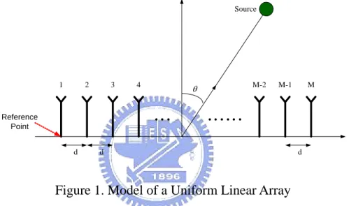
The array manifold vector is formed according to the array geometry and plane wave assumption of the sound signal. Take uniform linear array as the example,

Source d θ d

……

…

d Reference Point 1 2 3 4 M-2 M-1 M

Figure 1. Model of a Uniform Linear Array

Set the first microphone as the reference point, the array manifold vector of the linear array is defined as

sin ( 1) sin ( ) [1 j k dc j k d Mc ] T a θ = e ⋅ ⋅ ⋅ θ e ⋅ ⋅ ⋅ − ⋅ θ (2.20) where _c 2 c k π λ

= indicates the number of wave fronts, λ_c is the wave length, d is

the distance between adjacent microphones, and M is the number of microphones.

The ith element of the array manifold vector is the phase difference between the first microphone and the ith microphone when the source direction is θ . The phase difference in frequency domain is the temporal difference in time domain. Transform the array manifold vector to time domain will be

( ) [1 sin ( 1) sin ] T time domain c c d d a θ θ m θ λ λ − = ⋅ − ⋅ (2.21)

MUSIC calculates the inner product of the array manifold vector and 1( ), 2( ) ( )

d+ ωf d+ ωf M ωf

V V V to determine the direction of the source.

1 1 max ( ) ( ) DOA M H H i i i d a a θ θ θ = + ⎛ ⎞ ⎜ ⎟ ⎜ ⎟ = ⎜ _⋅⎛ _⋅ ⎞_⋅ ⎟ ⎜ ⎟ ⎜ _{⎝ ⎠} ⎟ ⎝

∑

V V ⎠ (2.22)

The signal subspace is orthogonal to noise subspace, so (2.20) could rewrite as

1 max ( ) ( ) d H H DOA i i i a a θ θ θ = ⎛ ⎛ ⎞ ⎞ = _{⎜ ⎜} ⋅ _{⎟ ⎟} ⎝ ⎠ ⎝

∑

V V ⎠ (2.23)

The array manifold vector represents the phase difference between microphones. Since MUSIC measures the projection of the array manifold vector to the signal subspace, the principle eigenvector of the signal subspace should contains the phase relation between microphones. So, we extract V1(ωf) from the signal subspace.

1(ωf)

V is the principle axis of the microphone array at frequency ω , and it could be f

expressed as 1( ) 11( ) 12( ) 1 ( ) T f V f V f VM f ω _{= ⎣}⎡ ω ω ω ⎤_⎦ V (2.24)

The principle matrix for all frequency is

11 1 11 2 11 12 1 12 2 12 1 1 1 2 1 ( ) ( ) ( ) ( ) ( ) ( ) ( ) ( ) ( ) F F M M M F V V V V V V V V V ω ω ω ω ω ω ω ω ω ⎡ ⎤ ⎢ ⎥ ⎢ ⎥ = ⎢ ⎥ ⎢ ⎥ ⎣ ⎦ 1 E (2.25)

In (2.25), the ith column is the principle vector at sound frequency ω . We i

ES-GCC between the ith microphone and the jth is defined as 1 * 1 1 ( ) F ( ) ( ) i j j x x Vi V j e d ω _ωτ ω τ =

∫

ω ω ω R (2.26)

And the estimation of the time delay between microphones is

ˆ arg max ( )

i j

ES GCC _τ x x

τ ₋ = R τ (2.27)

2.3 Performance of Different Eigenspace Methods in Real Time

Application

In this section we’ll discuss the functionality of ES-GCC and MUSIC. The time frame number required for ES-GCC to calculate a DOA is 1500*(200-1)+2560 samples, which is 18.82 sec. The MUSIC algorithm needs 2560*30 samples, which is 4.80 sec. So, ES-GCC is more time consuming. However, ES-GCC is able to calculate multiple sound sources without previous knowledge, while MUSIC is only able to estimate single source without other information. Another aspect is that ES-GCC requires a TDE step before estimating the direction, and MUSIC estimate the DOA directly. Since there might be TDE error in ES-GCC which causes more serious TDA estimation error, MUSIC is the method that has less estimation error. Finally, in the MUSIC algorithm the array manifold vector, which was determined by the array geometry, may not be a direct mapping with the source direction, so it’s computation consuming. On the other hand, ES-GCC only examines the delay relation between microphone pairs. It costs less computation to derive the DOA of the source.

Chapter 3. B

EARINGS

-O

NLY

SLAM A

LGORITHM

3.1 Between DOA estimation and Bearings-Only SLAM

The connection between DOA estimation algorithm and Bearings Only SLAM algorithm is essential. The DOA algorithm estimates the sound emitting direction of multiple sources. The output information may not be of the same index order, and the total number of estimated sound source is not static. The later algorithm should be able to handle incomplete measurement and unknown data association.

The Bearings-Only SLAM is a probabilistic robotics algorithm. It uses bearing information of landmarks in the environment to simultaneously localize the robot in the environment and to realize the location of the landmarks. The uncertain information from the output of DOA estimation algorithm is handled as the measurement input. The data association is not necessary to be known because the localization result based on wrong association is going to be eliminated using this algorithm. The remaining detail of Bearings-Only SLAM is introduced in the following section of this chapter.

3.2 Introduction of Probabilistic Robotics

Probabilistic robotics [6] is alternative to the conventional deterministic robotic. The key idea in probabilistic robotics is to represent uncertainty explicitly using the calculus of probability theory. Instead of relying on a single result as to what might be the case, probabilistic algorithm represents information by probability distributions over a whole space of guesses. They can represent ambiguity and degree of belief in a mathematically sound way. In contrast with traditional programming techniques in

robotics, probabilistic approaches tend to be more robust in the face of sensor limitations and model limitation. This enables them to scale much better to complex real-world environments than previous diagram, where uncertainty is of greater importance. Probabilistic algorithms are the only known working solutions to robotic estimation problems such as localization.

3.3 Bayes Filter

3.3.1 State Estimation using Probabilistic Generative Laws

Environments are characterized by state. The state is a collection of all information of the robot and its environment that can impact the future. It includes variables regarding to the robot itself, such as its pose, velocity, whether or not its sensors are functioning correctly, and so on. The robot uses its sensors to obtain information about the state of the environment, and the result of such perceptual interaction will be called measurement (or observation). The evolution of state and measurements is governed by probabilistic laws. Mathematically, the emergence of state xt is conditioned on all past states, measurement, and control inputs, so the

probability distribution of x_t could be expressed in the conditional probability form

0: 1 1: 1 1:

( _t | _t , _t , _t)

p x x ₋ z ₋ u (3.1)

where x0: 1t− are the past states from time index 0 to t− , 1 z1: 1t− are the past

measurements, and u_1:t are the past control input. Note that the control input u₁ is executed first, and then we take the measurement z₁. To simplify the expression, a state xt should be a sufficient summary of all that happened in previous time steps. In

this point of time, that is, u_{1: 1t−} and z_{1: 1t−} . So, if we already knew state x_t−1, only the control input ut will affect the present state. In mathematical expression

0: 1 1: 1 1: 1

( t | t , t , t) ( t | t , )t

p x x ₋ z ₋ u = p x x₋ u (3.2)

This property is called conditional independence.

Another key concept in the probabilistic robotics is belief. The belief is the robot’s internal knowledge about the state of the environment. Probabilistic robotics represents the beliefs through conditional probability distributions. Belief distributions are posterior probabilities over state variables conditioned on the available data. We denote belief over a state variable x_t by bel x( )_t

1: 1:

( )_t ( _t | _t, _t)

bel x = p x z u (3.3)

where the posterior is the probability distribution over the state xt at time t ,

conditioned on all past measurements z_1:t and all past control u_1:t. Notice that the belief is assumed to be taken after the measurement zt. If we take the belief before the

measurement, which is usually the case for real application, the posterior will be

1: 1 1:

( )t ( t | t , t)

bel x = p x z ₋ u (3.4)

This probability distribution is often referred to as prediction. The Bayes filter predicts the posterior bel x( )_t based on the previous state posterior bel x( _t−1), and then corporates bel x( )_t with the measurement at time t . The corporation is called measurement update.

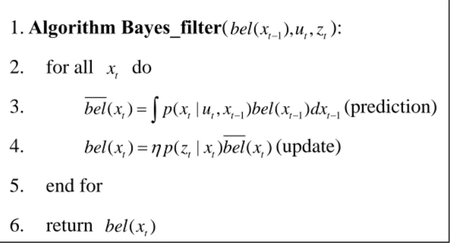
Figure 2. The Pseudo-Algorithm for Bayes Filtering

As in Figure 2, the Bayes filter algorithm possesses two essential steps. In line 3, it processes the control u_t. It does so by calculating a belief over the state x_t based on the prior belief over state x_t−1 and the control u_t. In particular, the belief bel x( )_t that the robot assigns to state xt is obtained by the integral (sum) of the product of

two distributions: the prior assigned to x_t−1, and the probability that control u_t

induces a transition from x_t−1 to x_t. This step is call predict.

The second step is update. In line 4, the Bayes filter algorithm multiplies the belief bel x( )t by the probability that the measurement zt may have been observed.

The result is normalized using η.

3.3.2 Parametric Filter – Kalman Filter and Extended Kalman Filter

The Kalman filter was invented by Swerling and Kalman [7] as a technique for filtering and prediction in linear Gaussian systems. The Kalman filter represents beliefs by the mean μ and covariance _t Σ , and the posteriors are Gaussian. The _t Kalman filter has several properties

1. Algorithm Bayes_filter(bel x( t−1), ,u zt t):

2. for all x_t do

3. bel x( )_t =

∫

p x u x( _t| _t, _t−1)bel x( _t−1)dx_t−1(prediction) 4. bel x( )_t =ηp z x bel x( |_{t t}) ( )_t (update)

5. end for 6. return bel x( )_t

1. The state transition probability p(x x_t | _t−1,u is a linear function with added _t) Gaussian noise. Which is

1

t = t t− + t t + t

x A x B u ε (3.5)

Here x and _t x are state vectors, and _t−1 u is the control vector at time t . _t The term ε is a Gaussian random vector that models the uncertainty _t generated by the state transition. Its mean is zero vector and covariance is R . t

So the total probability distribution is

1 1 1 1 ( | , ) 1 1 exp{ ( ) ( )} 2 | 2 | t t t T t t t t t t t t t t t t p π − − − − = − − − − − ⋅ x x u x A x B u R x A x B u R (3.6)

2. The measurement probability (p z_t |x is also a linear in the argument _t) transition.

t = t t + t

z C x δ (3.7)

The probability distribution of p z( t |x should be t)

1 ( | ) 1 1 exp{ ( ) ( )} 2 | 2 | t t T t t t t t t t t p π − = − − − ⋅ z x z C x Q z C x Q (3.8)

where Q is the covariance of the zero-mean Gaussian random vector t δt

3. The initial probability distribution of p x( ₀) is a Gaussian distribution. In this case the propagation of p x( )t is guaranteed to be Gaussian distribution.

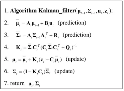
The above three characteristics are sufficient for the use of Kalman filter. Figure 3 is the detail algorithm procedure.

Figure 3. The Kalman Filter Algorithm for Linear Gaussian state transitions and measurements

After knowing the iterative procedure of Kalman filter, we now examine another version of Kalman filter, which is called EKF (extended Kalman filter). According to (3.5) and (3.7), the observations are linear functions of the state and the state transition is also linear function. This assumption is important to Kalman filter but not adequate for real world. The key point is that generally the transition and observation procedure of state are nonlinear functions. In mathematical form,

1 g( , ) t = t− t + t x x u ε (3.9) h( ) t = t + t z x δ (3.10)

Since the assumption we made about linear transition no longer exist, there should be some approximation about the nonlinear function. The most general terminology is linearization via first order Taylor expansion. Taylor expansion constructs a linear approximation to a function g from g ‘s value and slope near the function point. The slope is given by the partial derivative

1. Algorithm Kalman_filter(μt−1,Σt−1,u zt, t): 2. μ_t =A μ_{t t}−₁+B u_{t t} (prediction) 3. ₁ T t = _{t t− t} + _t Σ A Σ A R (prediction) 4. 1 ( ) T T t t t t t t t − = + K Σ C C Σ C Q 5. μ_t =μ_t+K z_t( _t−C μ_{t t}) (update) 6. Σ_t = −(I K C Σ_{t t}) t (update) 7. return μ Σ_t, _t

1 1 1 g( , ) g ( , ) : t t t t t − − − ∂ ′ = ∂ u x u x x (3.11)

From the expression above, g is approximated by its value at μ_t−1 and u_t, so

1 1 1 1 1 1 1 1 g( , ) g( , ) g ( , ) ( ) g( , ) ( ) t t t t t t t t t t t t t − − − − − − − − ′ ≈ + ⋅ − = + ⋅ − u x u μ u μ x μ u μ G x μ (3.12)

The matrix G is defined as the Jacobian matrix, and it should be a function of _t various value of μt−1 and ut . In the form of a Gaussian distribution, the state

transition probability distribution approximation is

1 1 1 1 1 1 1 1 ( | , ) 1 1 exp{ [ g( , ) ( )] 2 | 2 | [ g( , ) ( )]} t t t T t t t t t t t t t t t t t t p π − − − − − − − − = − − − ⋅ − ⋅ ⋅ − − ⋅ − x x u x u μ G x μ R R x u μ G x μ (3.13)

EKF implements the same linearization for the measurement function h . Here the Taylor expansion is developed around μ _t

h( ) h( ) h ( ) ( ) h( ) ( ) t t t t t t t t t ′ ≈ + ⋅ − = + ⋅ − x μ μ x μ μ H x μ (3.14)

The Gaussian form would be

1 ( | ) 1 1 exp{ [ h( ) ( )] 2 | 2 | [ h( ) ( )]} t t T t t t t t t t t t t t t p π − = − − − − ⋅ − − − z x z μ H x μ Q Q z μ H x μ (3.15)

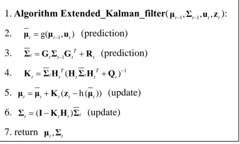
Figure 4. The Extended Kalman Filter Algorithm

Due to the simplicity and its computational efficiency, the EKF is almost the most frequently used state estimation terminology in robotics. Each update requires time

2.4 2

( )

O k +n , where k is dimension of the measurement vector z_t, and μ Σ_t, _t is the dimension of the state vector xt. Other algorithms, such as the particle filter, may

require time exponential in n

3.3.3 Nonparametric Filter - Particle Filter

Particle filter does not rely on a fixed functional form of the posterior, like Gaussian distribution in Kalman filter. It approximates posteriors by a finite number of values, each roughly corresponding to a region in state space. The quality of the approximation depends on the number of parameters used to represent the posterior. As the number of parameters goes to infinity, the method tends to converge uniformly to the correct posterior. The key idea is to represent the posterior bel x( )_t by a set of random state samples drawn from this posterior. In particle filters, the samples of a posterior distribution are called particles.

1. Algorithm Extended_Kalman_filter(μt−1,Σt−1,u zt, t): 2. μ_t =g(μ_t−₁,u_t) (prediction) 3. ₁ T t = _{t t− t} + _t Σ G Σ G R (prediction) 4. 1 ( ) T T t t t t t t t − = + K Σ H H Σ H Q 5. μ_t =μ_t+K z_t( _t−h ( ))μ_t (update) 6. Σ_t = −(I K H Σ_{t t}) t (update) 7. return μ Σ_t, _t

[1] [2] [ ]

: , , , M

t = t t t

χ x x x (3.16)

Each particle x_t[ ]m is a representation of the state at time t . In other words, a particle is a hypothesis as to what the true world state may be at time t . M is the

number of particles in the particle set χ . Ideally, the likelihood for a state to be _t included in the particle set χ shall be proportional to its posterior t bel x( )t

[ ] 1: 1: ( | , ) m t p t t t x ∼ x z u (3.17)

Just like all other Bayes filter algorithms discussed, the particle filter algorithm constructs the belief bel x( )_t recursively from the bel x( _t−1) one time step earlier, which means the particle set χ recursively from the set _t χ . The input of particle _t−1 filter is the particle set χ , along with the most recent control _t−1 u and the most _t recent measurement z . To get the predicted probability distribution _t bel x( )_t , we sample the new particles x_t[ ]m according to the distribution of the previous step

1

( _t | _t, _t )

p x u x₋ . To incorporate the measurement z into the particle set, we calculate _t the importance factor wt[ ]m , which are obtained according to the probability of the

measurement z under particle _t x_t[ ]m , given by w_t[ ]m = p(z x_t | _t[ ]m ). If we interpret

[ ]m t

w as the weight of a particle, the set of weighted particles represent approximately the Bayes filter posterior bel x( )_t . The last step is called resample. Since each of the particles already has a corresponding weight, the weigh value could be interpreted as the probability that this particle would be chosen again. Resampling algorithm transforms a particle set of M particles into another particle set of the same size. Before the resampling step, they were distributed according to bel x( )_t , after the

resampling the dare distributed according to the posterior

[ ]

( )_t ( _t | _t m ) ( )_t

bel x =ηp z x bel x . The illustrated algorithm flow is in Figure 5.

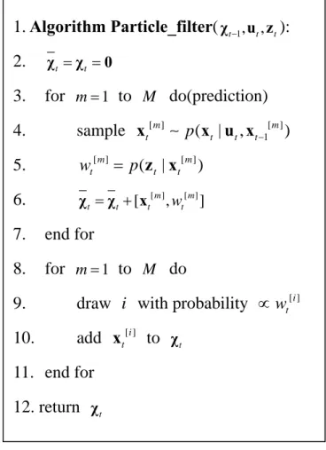
Figure 5. The Particle Filter Algorithm, a Bayes Filter Based on Importance Sampling

3.4 SLAM

3.4.1 Problem Definition

The simultaneous localization and mapping problem is commonly abbreviated as

SLAM, and is also known as Concurrent Mapping and Localization. SLAM problem

arise when the robot does not have access to a map of the environment, nor doest it know its own pose. All it is given are measurement z1:t and controls u1:t. In SLAM,

the robot acquires a map of its environment while simultaneously localizing itself 1. Algorithm Particle_filter(χt−1,u zt, t): 2. χ_t =χ_t =0 3. for m=1 to M do(prediction) 4. sample [ ] ( | , 1[ ]) m m t p t t t− x ∼ x u x 5. w_t[ ]m = p(z x_t | _t[ ]m ) 6. [ ] [ ] [ _tm, _tm] t = +t w χ χ x 7. end for 8. for m=1 to M do

9. draw i with probability ∝wt[ ]i

10. add x to t[ ]i χt

11. end for 12. return χt

relative to this map. From a probabilistic perspective, there are two main forms of the SLAM problem, which are both of equal practical importance. The online SLAM estimates the posterior over the momentary pose along with the map.

1: 1:

( ,t | t, t)

p x m z u (3.18)

where x_t is the pose at time t, m is the map. This problem is call online SLAM problem since it only involves the estimation of variables that persist at time t. The other category is called the full SLAM. In full SLAM, we calculate a posterior over the entire path x1:t along with the map, instead of just the current pose xt.

1: 1: 1:

( t, | t, t)

p x m z u (3.19)

The mathematical relation between (3.18) and (3.19) is shown below.

1: 1: 1: 1: 1: 1 2 1

( ,_t | _t, _t) ( _t, | _t, _t) _t

p x m z u =

∫∫ ∫

p x m z u d dx x …dx₋ (3.20) In practice, calculating a full posterior like (3.19) is usually infeasible. Problems arise from the high dimensionality if the continuous parameter space, and the large number of discrete correspondence variables. Many state-of-the-art SLAM algorithms construct maps with tens of thousands of features, or more. Even under known correspondence, the posterior over those maps alone involves probability distributions over space with 105 or more dimensions. This is opposite to localization problems, in which posteriors were estimated over three-dimensional continuous spaces. Not to say in most application the correspondence are unknown. The number of possible assignments to the vector of all correspondence variables grows exponentially. Thus practical SLAM algorithms that can cope with the correspondence problem must rely on approximations.

3.4.2 FastSLAM

FastSLAM is a combinational algorithm that is using both the concept of particle filter and the extended Kalman filter. Particle filters are at the core of some of the most effective robotics algorithm. However the particle filter is not so applicable to the SLAM algorithm due to the course of dimensionality, it scales exponentially with the number of dimensions of the estimation problem. A straightforward implementation of particle filters for the SLAM problem would fail because of the large number of variables involved on describing a map.

In a SLAM problem with known correspondence, there is a conditional independence between any two disjoint set of features in the map, given the robot pose. So we could estimate the location of all features independently of each other. Dependencies on these estimates arise only through robot pose uncertainty. This structural characteristic makes it possible to apply Rao-Blackwellized Particle Filter (RB particle filter) to SLAM problem. RB particle filter uses particles to represent the posterior over some variables, along with parametric PDF to represent all other variables.

We use particle filter to estimate the robot path. Since the conditional independent characteristic holds, the mapping problem can be factored into many separate problems, one for each feature in the map. Each single map feature is estimated using a low-dimensional EKF. This is different from other SLAM algorithms that use single high-dimensional Gaussian to estimate the all features jointly.

The advantage of FastSLAM is that it could be implemented in time logarithmic in the number of features, so it’s computational efficient. Another key advantage of

FastSLAM is that the data association decisions can be made on per-particle basis. The ability to pursue multiple data associations simultaneously makes FastSLAM significantly more robust to data association problems than algorithms based on incremental maximum likelihood data association.

robot path feature 1 feature 2 feature N

Particle 1 k = [1] [1] 1: {( , , ) }1: T t = x y θ t x [1] [1] 1 , 1 μ Σ [1] [1] 2 , 2 μ Σ [1] [1] , N N μ Σ Particle 2 k= [2] [2] 1: {( , , ) }1: T t = x yθ t x [2] [2] 1 , 1 μ Σ [2] [2] 2 , 2 μ Σ [2] [2] , N N μ Σ Particle k =M [ ] [ ] 1: {( , , ) }1: M T M t = x yθ t x [ ] [ ] 1 , 1 M M μ Σ [ ] [ ] 2 , 2 M M μ Σ [ ] [ ] , M M N N μ Σ

Table 1. Particles in FastSLAM are composed of a path estimate and a set of estimators of individual feature locations with associated covariance Particles in the basic FastSLAM algorithm are of the form shown in Table 1. Each particle contains an estimated robot pose, denoted [ ]

1:

k t

x , and a set of Kalman filters with mean [ ]k

j

μ and covariance [ ]k j

Σ , one for each feature m_j in the map. Here [ ]k

is the index of the particle. As usual, the total number of particles is denoted M . The basic step of the FastSLAM includes several steps. At each time step t , retrieve a pose 1[ ]

k t−

x from the particle set, sample a new pose according to the distribution

[ ] [ ]

( | , )

k k

t p t t t

x ∼ x x u . Then for each observed feature z_tj, identify the correspondence

j and update the corresponding EKF by updating mean ,[ ]

k j t μ and covariance ,[ ] k j t Σ .

Each new particle should have a new importance weight w[ ]k . The final step is resample, which is sampling the M particles with the probability proportional to

[ ]k

3.4.3 Unknown Data Association

The data association is also mentioned as correspondence in this thesis. In most

of the Bayes filter process, the data association problem exists. Every time we take a measurement of the map, we don’t necessarily know which feature the measurement belongs to (usually we don’t have this piece of information). Generally the data association techniques are using argument such as maximum likelihood. They have only single data association per measurement for the entire filter, and once the association is incorrect, the update procedure fails and the filter diverges. The key advantage of using particle filters for SLAM is that each particle can rely on its own, local data association decision. Thus, the filter is actually sampling over possible data association decisions. Since there are multiple correspondence decisions, as long as a small subset of the particles is based on the correct data association, data association errors are not as fatal as in EKF approaches. Particles with wrong correspondence will possess inconsistent map, which decrease the weight of those particles, and hence they are more likely to be sampled out in the future resample step.

3.5 Simulation Result of Fast SLAM

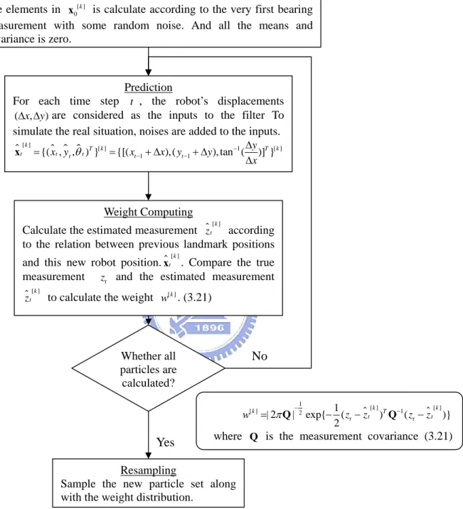
In this simulation we’ll examine the effectiveness of the FastSLAM algorithm. Assume there are 6 features in the environment that are to be tracked, and the robot will walk through a certain path that is previously given. The space is 700cm*700cm. Maximum detectable range of the bearing sensors is 300cm. The algorithm generates particles according to the very first bearing measurements. Since there is a maximum detectable range, we sample the initial particle ranges according to a uniform distribution of half of the maximum range. The procedure is as Figure 6.

Figure 6. The Simulation Procedure of the FastSLAM Algorithm

Notice that in (3.21), the weight value will be small if the estimated measurement is different from the real measurement. And since there is resample step, we don’t have to worry about data association problem.

Initialization

Each particle is a state vector of robot pose and landmark estimation.

[ ] [ ] [ ] [ ] [ ] [ ] [ ] [ ] 0 { 0 , 1.0 , 1,0 , 2,0 , 2,0 , , ,0 , ,0 } k k k k k k k k N N μ μ μ = Σ Σ Σ Y x where [ ] [ ] 0 {( , , ) }0 k T k x yθ = x The elements in [ ] 0 k

x is calculate according to the very first bearing measurement with some random noise. And all the means and covariance is zero.

Prediction

For each time step t , the robot’s displacements

(Δ Δx, y)are considered as the inputs to the filter To simulate the real situation, noises are added to the inputs.

[ ] [ ] 1 [ ] 1 1 {( , , ) } {[( ),( ), tan ( )] } k T k T k t t _t t _{t t} y x y x x y y x θ − − − Δ = = + Δ + Δ Δ x Weight Computing

Calculate the estimated measurement zt[ ]k according

to the relation between previous landmark positions and this new robot position.xt[ ]k . Compare the true

measurement zt and the estimated measurement

[ ]k t

z to calculate the weight [ ]k

w . (3.21)

Whether all particles are calculated?

Resampling

Sample the new particle set along with the weight distribution.

Yes No 1 [ ] [ ] [ ] ₂ 1 1 | 2 | exp{ ( ) ( )} 2 k k k T t t t t w = πQ− − z −z Q− z −z

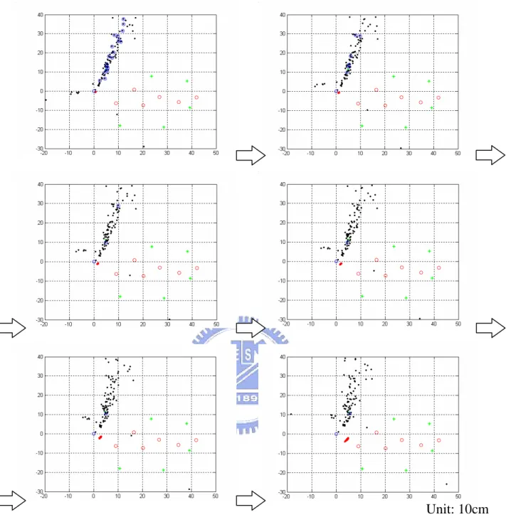
Unit: 10cm Figure 7. Simulation Results of the FastSLAM Algorithm without Resample

(Only single feature is illustrated)

Figure 7 shows a sequential graph of the simulation. The six green stars are the feature that to be localized. Red dots are the estimation of the current robot position. Red circles are the waypoint of the path. All the black particles are trying to localize the feature at (4.95,11.26). And the blue circles are the particles with larger weight value (there is also a blue circle at the origin). To explain what the figure is all about,

we conclude the following observation. Originally there are a lot of particles that have high weight, and as time step increase, the weight will concentrate to several mostly correct particle. Even if the resample state is not implemented, the outlier particles will converge to the feature’s neighborhood.

Unit: 10cm Figure 8. Simulation Results of the FastSLAM Algorithm with Resample

In Figure 8, it is shown that with the help of resample, all the low-weight particles will be sampled out. The filter converges in only few time steps.

Chapter 4. Experimental Result and Discussion

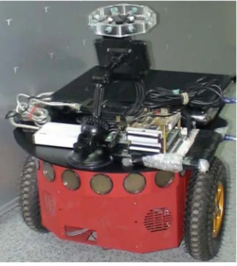
4.1 Introduction of the Robot Platform

In the experimental results presented afterward, we’re using a research and development platform called PIONEER 3-DX from MobileRobots Inc. Some detail specification is written in Table 2.

Pioneer 3-DX Research Robot

Length 44.5 cm Width 40.0 cm Height 24.5 cm Physical Weight (with battery) 9 kg

Battery 12V sealed, lead-acid

Charge Time 12 hours

Power

Run time 18-24 hours

Drive 2-wheel drive, plus rear balancing caster

Gear ratio 38.3:1

Pushing force 6 kg

Swing radius 32 cm

Mobility

Translate speed max 1.2 m/sec

Standard position encoders 500 tick encoders

Communications ports 3 RS-232 serial ports on microcontroller Main power switch Robot power; 12VDC; red LED indicator

Table 2. The Specification of the POINEER 3-DX Robot [9]

The main purpose of using this robot platform is to record the robot path using the included position encoders. These encoder data will be considered as the input to the FastSLAM algorithm. We use a laptop to control the robot through the RS-232 port. A wireless access point in mounted on the robot so that the instruction could be done remotely.

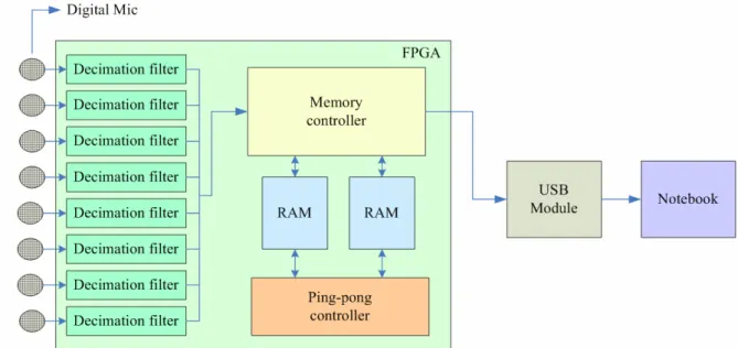
Another important hardware is the microphone array. Figure 10 shows the architecture of the array, which contains 8 digital microphones, an FPGA, and the USB communication module. The digital microphones are using the MEMS technology to imbed sigma-delta modulators in the microphones. Digital microphones have the advantages of little signal crosstalk, low circuit noise, and small circuit size due to needless of A/D converter. The FPGA will take decimation to the microphone input data. It passes the 1.2MHz digital microphone signal through a second-order low pass filter (LPF), and down samples the 1.2 MHz 75 times to get a 16 KHz sound signal. Afterward, the USB will select the channel number through a MUX, and simultaneously transmit the 8-channel 16 KHz data to the laptop.

(a) (b)

Figure 11. (a) The 8-Channel Digital Microphone (b) The FPGA and the USB Module The experimental data was recorded in a 350cm*450cm room, with three static loud speakers playing human speech in English. The circular microphone array is of radius 5.5cm, so the far field assumption hold since the scale ratio between the room size and the array size is large enough. The robot is waking through a specifically design path to avoid some improper situations for DOA estimation and Bearings-Only SLAM. Figure 12 shows the environment that we record the sound data.

Figure 12. The Spatial Relation of the Speaker, the Robot, and the Laser Range Finder

4.2 Performance of offline calculated algorithm

The experiment was first done under an offline calculation to test the algorithm effectiveness. The program procedure for offline calculated FastSLAM is shown in

Figure 13. The Algorithm Procedure for Offline Calculation

As mentioned in section 2.3, the ES-GCC method estimates the DOA by using the least square method. The algorithm needs to accumulate a certain time frame to get solid delay information between microphones. Only those delay combination with reasonable sound speed generates DOA estimation. Furthermore, the DOA estimation is not necessary correct, which may be eliminated in the Outlier Elimination step. Upon all the reasons above, the DOA estimation won’t be correct when the robot is

DOA Estimation

At every time step, the ES-GCC algorithm might calculates several outputs representing the sound sources direction.

Outlier Elimination

Occasionally the DOA estimated by ES-GCC has unreasonable value. To determine whether the value is an outlier, we compare the previous and present robot position to define a reasonable DOA range.

Weight Computing

Without need of calculating correspondence, all the particles should compare their estimated feature measurement with the DOA result and evaluated the weight of them.

Whether all particles are calculated?

Resampling

Sample the new particle set along with the weight distribution.

Yes

moving. So we program the algorithm to update the estimation only when the robot stops. The experimental results are shown below.

Figure 14. The Experimental Results of Offline Calculated FastSLAM

In Figure 14, the blue ground truth data are collected by a static laser range finder to compare the SLAM output and the real environment. The big yellow clusters are the waypoints that the robot stops to update the landmark estimation.

Landmark 1 Landmark 2 Landmark 3 Average

Range Error 5 cm 22 cm 6cm 11cm

Range Error Rate 2.05% 7.90% 1.81% 3.92%

Bearing Error 2.81 4.48 5.03 4.11

Table 3. The Error Analysis of Offline Calculated FastSLAM

As in Table 3, the position estimation has larger error rate than the landmarks estimation. This phenomenon happens due to the joint uncertainty of the feature estimation and the encoder measurement. Conceptually, the position estimation is a sensor fusion result of the encoder and the DOA measurement. To adjust the believe ratio between DOA measurement and encoder, the covariance matrix of these two

● ground truth

● encoder location

● estimated robot location

● estimated landmark (mean)

sensor data should be modified.

4.3 Performance of online algorithm

The online algorithm here is not identical to the online SLAM mentioned in section 3.3. Here the “online” stands for the issue for real-time experiment. Some modifications of the FastSLAM algorithm are made for this application. The most significant adjustment is the removal of the resample state.

Figure 15. The Algorithm Procedure for Onine Calculation

The pseudo procedure of the real-time experiment is illustrated in Figure 15. In order to release the calculation load of particle filter, the number of particles is decreased. Theoretically there is still a subset of the particle that is still having the

DOA Estimation

At every time step, the MUSIC algorithm calculates one output representing one sound sources direction. The bearing measurements might belong to different landmarks

Data Accumulation and Voting

Use the nearest neighborhood concept to sort the MUSIC output into categories. The categories with large number of votes are considered to be sound source. The output of this stage may be multiple directions.

Particle Update

Associate the measurement with the nearest neighborhood (estimation) and update the particle using this correspondence information.

Particle Initialization

Assume all the features exist and are emitting sound at the beginning of the scenario. The accumulated MUSIC initializes all the particles with the features it detected.

right correspondence. However, based on our experiment that this subset would not always exist, and hence the resample state will be forced to choose a wrong data association that is having relatively higher weight. This will fail the whole filter procedure.

Another adjustment is the DOA estimation method. We use the accumulated MUSIC to estimate the DOA instead of ES-GCC. MUSIC has a very good characteristic in finding single source. Under the situation of multiple speech sources with same scale of magnitude, MUSIC tends to find each of them sequentially. So, by accumulating the calculated directions, we sort this array using nearest neighborhood method. Only the clusters with sufficient amount DOA estimation pass through this step. The output of this step would be a robust DOA estimation.

Figure 16. The Real-time Experimental Environment

Figure 16 shows how the speaker is distributed. The robot considers its start point as the origin and move through a path that doesn’t have severe echo problem and

sound source overlap. We use 30 particles to describe the probability distribution.

Figure 17. The Real-time Experimental Results

The red circle in Figure 17 is the robot position estimation. The yellow, light blue and blue circles are the distributed particles. The red crosses are the mean of each group of estimation, and the green square is the ground truth of the features.

step, so three sets of particles were initialized. As the robot stopped at the next stop point, the accumulated MUSIC popped out one angle value. This angle was recognized to be a measurement of landmark 3. So the filter updated the estimation of landmark 3 for a while and headed to the next stop point. Afterward, the measurement of landmark 1 and 2 popped out. The filter was able to update arbitrary numbers of estimation group.

Landmark 1 Landmark 2 Landmark 3 Average

Range Error 50 cm 2 cm 3 cm 18.33 cm

Range Error Rate 16.27% 0.70% 1.67% 6.21%

Bearing Error 1.74 2.82 4.76 3.11

Table 4. The Error Analysis of Real-time FastSLAM

As in Table 4, the average range error rate is 6.21%, and the average bearing error is 3.11 . The final result of the real-time FastSLAM is illustrated in Figure 18.

Figure 18. The Final Real-time Experimental Results 180 cm

170 cm

Chapter 5. Conclusion and Future Study

A combinational algorithm of DOA estimation and Bearings-Only SLAM is proposed in this thesis. The new algorithm is managed to deal with the landmark occlusion problem commonly faced in vSLAM. Using the ES-GCC or accumulative MUSIC allows us to estimate multiple DOAs within a short period of time frame. The theoretical knowledge of SLAM is presented in chapter 3 to explain the nondeterministic method that is used in the thesis. Figure 7 and figure 8 shows the simulation results of a particle filter.

The experimental result presented in chapter 4 show that the algorithm is applicable in offline calculation. Due to some hardware limitation, the real-time calculation procedure neglects the resampling part of the original algorithm and applies the nearest neighborhood concept to the data association. The simultaneous localization and mapping results are shown with range error of 6.21% and bearing error of 3.11 in average.

There are several areas for improvement. The more particles that are used in a particle filter, the more accurate it is. The real-time process could be modified in other method rather than decreasing the particle number. Also, the experiment in this thesis assumes that all the landmarks could be detected in the initial state. If there are new landmarks, the current algorithm is not able to localize them. An adjustable state vector should be used to intelligently modify the size of the vector to improve the SLAM robustness. Also, although the sound sources are detectable when they are NLOS, the DOA information does not hold the same characteristic. The specificity of NLOS sound sources should be studied.