利用Ritz法分析具有V型缺口之矩形薄板振動
101
0
0
全文
(2) 利用 Ritz 法分析具有 V 型缺口之矩形薄板振動 研究生︰廖慎謙. 指導教授︰黃炯憲. 博士. 國立交通大學土木工程學系碩士班 摘. 要. 應力奇異點之問題常發生於工程力學的分析計算中。本論文以薄 板理論為基礎,利用 Ritz 法分析具有 V 型缺口之矩形板振動,在分 析過程中使用兩組允許函數序列,分別為:(1)多項式函數,其本身 可構成一組完備之序列;(2)角函數,滿足 V 型缺口兩自由邊緣之邊 界條件,並可精確地描述缺口尖端之應力奇異特性。本論文之研究案 例包含完全自由與懸臂矩形板,先以完整的收斂性分析驗證角函數能 夠有效地加速自然振動頻率之收斂速度,並探討不同幾何及位置之 V 型缺口對矩形板振動行為之影響。本論文為首次研究具有 V 型缺口 之矩形板振動,此研究結果可提供後人研究參考與比較。. i.
(3) Vibrations of Rectangular Thin Plates with a V-notch via the Ritz Method Student︰Shen-Chien Liao. Adviser︰Dr. Chiung-Shiann Huang. Department of Civil Engineering National Chiao-Tung University Abstract This thesis presents a novel method for accurately determining the natural frequencies of rectangular plates with an edge V-notch. Based on the well-known Ritz method, two sets of admissible functions are used simultaneously: (1) algebraic polynomials, which form a complete set of functions; (2) corner functions, which are the general solutions of bi-harmonic equation, duplicate the boundary conditions along the edges of the notch, and describe the stress singularities at the sharp vertex of the V-notch exactly. The rectangular plates under consideration are either completely free or cantilevered. The effects of corner functions on the convergence of solutions are demonstrated through comprehensive convergence studies. Accurate numerical results and nodal patterns are tabulated for V-notched plates having various notch angle, depths and locations. These are the first known frequency and nodal pattern results of V-notched rectangular plates in the published literature.. ii.
(4) Acknowledgements For the accomplishment of the Master’s thesis, I would like to express my sincere appreciation to my advisor, Professor C. S. Huang. He supports me not only the guidance for the study work but also the beneficial knowledge and techniques for research. I would also thank my thesis committees, Professor G. S. Liou, Professor S. L. Hung and Professor F. P. Cheng for their constructive comments and suggestions on the thesis. During graduate school, I am indebted to my seniors, M. J. Chang and W. C. Su. Acknowledgements go to their great help in my school life and academic work. I would like to thank my classmates in laboratory, C. D. Yang, C. W. Chan and Y. S. Wei, for their cooperation with me. I also thank my seniors, S. Y. Lo, C. Y. Lin and T. W. Hsu for their assistance. I wish to treasure the pleasant memories in NCTU graduate school. Acknowledgements also go to the supports in figure plotting from my classmates in undergraduate school, P. H. Ho and H. W. Yu. I am thankful to my roommates, Y. C. Lee and C. C. Liu, for their favors. Finally, my parents and both my sisters are gratefully acknowledged. No words can express my appreciation to their invaluable supports and encouragements. Shen-Chien Liao July 16, 2007. iii.
(5) Table of Contents Abstract in Chinese ..................................................................................... i Abstract in English..................................................................................... ii Acknowledgements................................................................................... iii Table of Contents ...................................................................................... iii List of Tables............................................................................................ vii List of Figures .............................................................................................x Chapter 1. Introduction .............................................................................1. 1.1 Research Background ....................................................................1 1.2 Literature Review...........................................................................2 1.3 Contents in the Thesis ....................................................................5 Chapter 2. Corner Functions and Stress Singularities ..............................6. 2.1 Corner Functions and Characteristic Equations ............................6 2.2 Stress Singularities at Corners .....................................................11 Chapter 3. Vibrations of Completely Free Rectangular Plates...............13. 3.1 Formulation for the Ritz method .................................................13 3.2 Admissible Functions...................................................................14 3.3 Convergence Study ......................................................................16 3.4 Numerical Results........................................................................20 iv.
(6) Chapter 4. Vibrations of Cantilevered Rectangular Plates .....................25. 4.1 Admissible Functions...................................................................25 4.2 Convergence Study ......................................................................25 4.3 Numerical Results........................................................................29 Chapter 5. Concluding Remarks.............................................................32. References.................................................................................................32. v.
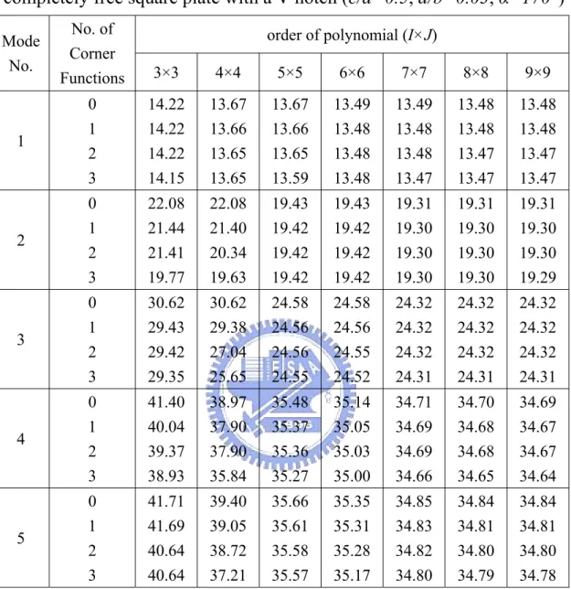
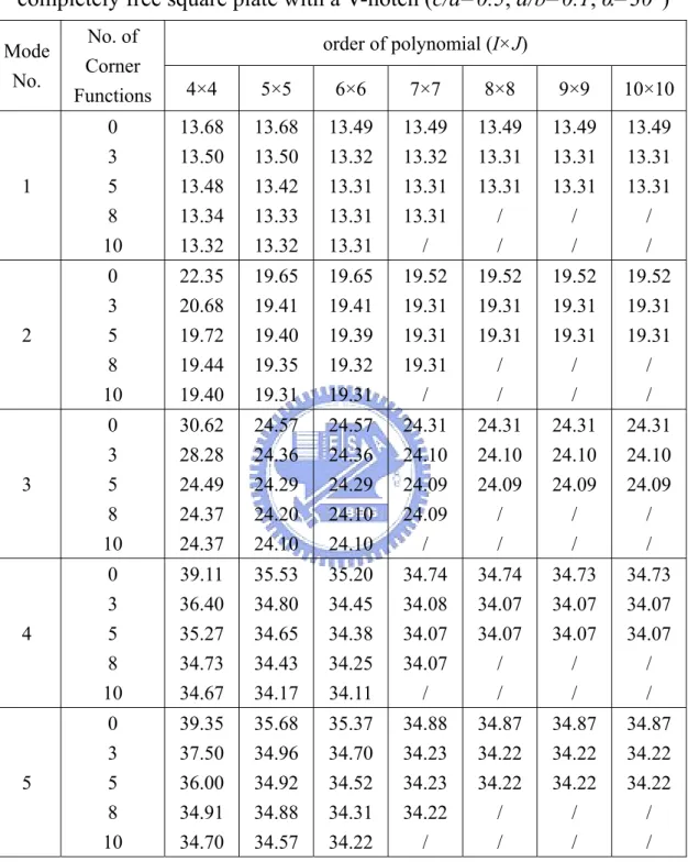
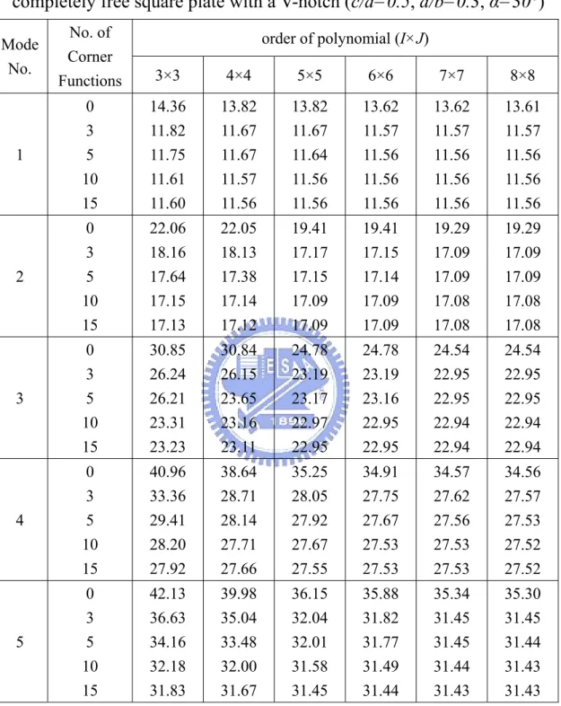
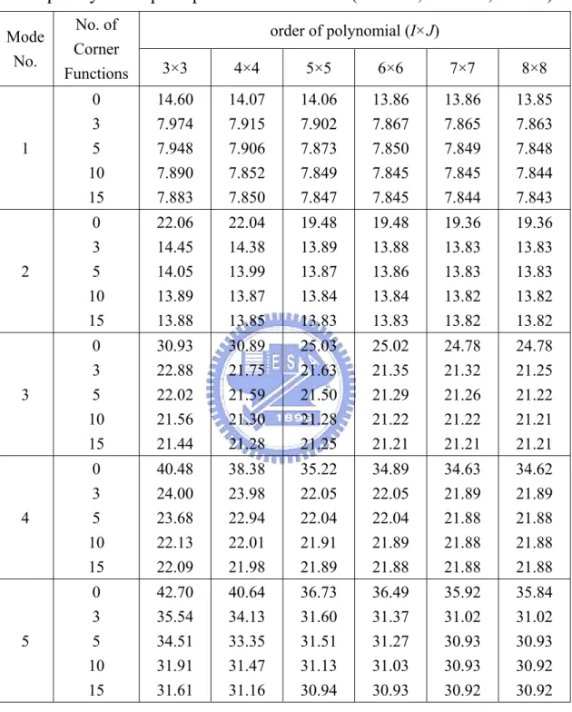
(7) List of Tables Table 3.1 Convergence of frequency parameters ωa 2 ρh / D for a completely free square plate .....................................................37 Table 3.2 Convergence of frequency parameters ωa 2 ρh / D for a completely free square plate with a V-notch (c/a=0.5, d/b=0.03, α=170°).....................................................................................38 Table 3.3 Convergence of frequency parameters ωa 2 ρh / D for a completely free square plate with a V-notch (c/a=0.5, d/b=0.1, α=30°).......................................................................................39 Table 3.4 Convergence of frequency parameters ωa 2 ρh / D for a completely free square plate with a V-notch (c/a=0.5, d/b=0.3, α=30°).......................................................................................40 Table 3.5 Convergence of frequency parameters ωa 2 ρh / D for a completely free square plate with a V-notch (c/a=0.5, d/b=0.5, α=30°).......................................................................................41 Table 3.6 Convergence of frequency parameters ωa 2 ρh / D for a completely free square plate with a V-notch (c/a=0.5, d/b=0.5, α=5°).........................................................................................42 Table 3.7 Convergence of frequency parameters ωa 2 ρh / D for a completely free square plate with a V-notch (c/a=0.5, d/b=0.3, vi.
(8) α=0°).........................................................................................43 Table 3.8 Frequency parameters ωa 2 ρh / D for a completely free rectangular plates with a V-notch (a/b=1.0, υ=0.3) .................44 Table 3.9 Frequency parameters ωa 2 ρh / D for a completely free rectangular plates with a V-notch (a/b=2.0, υ=0.3) .................45 Table 3.10 Frequency parameters ωa 2 ρh / D for a completely free rectangular plates with a V-notch (a/b=0.5, υ=0.3) ...............46 Table 3.11 Relative reductions of the frequency parameters for Δωn completely free rectangular plates with a V-notch (a/b=1.0, υ=0.3)......................................................................................47 Table 3.12 Relative reductions of the frequency parameters for Δωn completely free rectangular plates with a V-notch (a/b=2.0, υ=0.3)......................................................................................48 Table 3.13 Relative reductions of the frequency parameters for Δωn completely free rectangular plates with a V-notch (a/b=0.5, υ=0.3)......................................................................................49 Table 4.1 Convergence of frequency parameters ωa 2 ρh / D for a cantilevered square plate...........................................................50 Table 4.2 Convergence of frequency parameters ωa 2 ρh / D for a cantilevered square plate with a V-notch (c/a=0.5, d/b=0.03, vii.
(9) α=170°).....................................................................................51 Table 4.3 Convergence of frequency parameters ωa 2 ρh / D for a cantilevered square plate with a V-notch (c/a=0.5, d/b=0.1, α=30°).......................................................................................52 Table 4.4 Convergence of frequency parameters ωa 2 ρh / D for a cantilevered square plate with a V-notch (c/a=0.5, d/b=0.3, α=30°).......................................................................................53 Table 4.5 Convergence of frequency parameters ωa 2 ρh / D for a cantilevered square plate with a V-notch (c/a=0.5, d/b=0.5, α=30°).......................................................................................54 Table 4.6 Convergence of frequency parameters ωa 2 ρh / D for a cantilevered square plate with a V-notch (c/a=0.5, d/b=0.3, α=5°).........................................................................................55 Table 4.7 Convergence of frequency parameters ωa 2 ρh / D for a cantilevered square plate with a straight crack (c/a=0.5, d/b=0.25, α=0°, h/a=1/80, υ=0.33) .........................................56 Table 4.8 Frequency parameters ωa 2 ρh / D for cantilevered rectangular plates with a V-notch (a/b=1.0, υ=0.3) ....................................57 Table 4.9 Frequency parameters ωa 2 ρh / D for cantilevered rectangular plates with a V-notch (a/b=2.0, υ=0.3) ....................................58. viii.
(10) Table 4.10 Frequency parameters ωa 2 ρh / D for cantilevered rectangular plates with a V-notch (a/b=0.5, υ=0.3) ...............59 Table 4.11 Relative reductions of the frequency parameters Δωn for cantilevered rectangular plates with a V-notch (a/b=1.0, υ=0.3) .................................................................................................60 Table 4.12 Relative reductions of the frequency parameters Δωn for cantilevered rectangular plates with a V-notch (a/b=2.0, υ=0.3) .................................................................................................61 Table 4.13 Relative reductions of the frequency parameters Δωn for cantilevered rectangular plates with a V-notch (a/b=0.5, υ=0.3) .................................................................................................62. ix.
(11) List of Figures Fig. 2.1 Stress resultants in polar coordinate............................................63 Fig. 2.2 A sectorial plate ...........................................................................64 Fig. 2.3 The coordinate system defined in a sectorial plate .....................65 Fig. 2.4 Variation of minimum Re(λn) with vertex angle α......................66 Fig. 3.1 The coordinate system defined in a completely free rectangular plate with a V-notch ....................................................................67 Fig. 3.2 Nodal patterns for completely free square plates with a V-notch at c/a=0.5 ........................................................................................68 Fig. 3.3 Nodal patterns for completely free square plates with a V-notch at c/a=0.75......................................................................................69 Fig. 3.4 Nodal patterns for completely free rectangular plates (a/b=2.0) with a V-notch at c/a=0.5 ...........................................................70 Fig. 3.5 Nodal patterns for completely free rectangular plates (a/b=2.0) with a V-notch at c/a=0.75 .........................................................72 Fig. 3.6 Nodal patterns for completely free rectangular plates (a/b=0.5) with a V-notch at c/a=0.5 ...........................................................74 Fig. 3.7 Nodal patterns for completely free rectangular plates (a/b=0.5) with a V-notch at c/a=0.75 .........................................................76 Fig. 3.8 superposition of the fifth and forth mode shapes for completely free square plates ........................................................................78 x.
(12) Fig. 4.1 The coordinate system defined in a cantilevered rectangular plate with a V-notch.............................................................................79 Fig. 4.2 Nodal patterns for cantilevered square plates with a V-notch at c/a=0.5 ........................................................................................80 Fig. 4.3 Nodal patterns for cantilevered square plates with a V-notch at c/a=0.75......................................................................................81 Fig. 4.4 Nodal patterns for cantolevered rectangular plates (a/b=2.0) with a V-notch at c/a=0.5 ...................................................................82 Fig. 4.5 Nodal patterns for cantilevered rectangular plates (a/b=2.0) with a V-notch at c/a=0.75 .................................................................84 Fig. 4.6 Nodal patterns for cantilevered rectangular plates (a/b=0.5) with a V-notch at c/a=0.5 ...................................................................86 Fig. 4.7 Nodal patterns for cantilevered rectangular plates (a/b=0.5) with a V-notch at c/a=0.75 .................................................................88. xi.
(13) Chapter 1. Introduction. 1.1 Research Background Plate structures are very common in engineering practice, and are extensively used in civil, mechanical, and aeronautical engineering, such as concrete floor slab and aircraft skin components. Their vibrational behaviors have caught great interests of many researchers. Stress singularities mean that infinite stresses exist at some points in the domain under consideration, and are often encountered in plate problems. Three main reasons causing stress singularities are: (1) discontinuousness of geometry, such as cracks in the domain or sharp re-entrant angles at the boundary; (2) concentrated loads, such as point forces or moments; (3) suddenly change of material properties, such as composite material. When the stress singularity behaviors exist in the domain under consideration, it is necessary to find the asymptotic solutions, which can exactly describe the stress singularities, for obtaining accurate solutions for static or vibration problems. However, as the demand for engineering structures is improving, a singularity problem is unavoidable in engineering analysis. Vibrations of V-notch plates are concerned with stress singularity problems due to the sharp vertex. Such notches may be generated intentionally in the plate for clearance or other reasons. This thesis utilizes the well-known Ritz method to analyze the vibration of rectangular plates with a V-notch based on the classical plate theory. Two 1.
(14) sets of admissible functions are used in the analysis method simultaneously: (1) algebraic polynomials, which form a complete set of functions; (2) corner functions, which are the general solutions of bi-harmonic equation, duplicate the boundary conditions along the edges of the notch, and describe the stress singularities at the sharp vertex of the V-notch exactly. The rectangular plates under consideration are completely free and cantilevered, respectively. The effects of the asymptotic solutions on the convergence of numerical solutions are demonstrated through convergence studies. The efftects of the V-notch on the vibration behaviors of rectangular plates also are discussed in detail.. 1.2 Literature Review On the topic of plate vibrations, at least 2000 research papers have been published. Leissa (1967) summarized the methods of analysis and numerical results found in 500 references on the free vibration of plates published before 1967 in his classical monograph. Since then, research and publication on this subject has been at an increasing rate. In these studies, vibration of cracked plates is a problem of greatest interests, which combines the fields of vibration analysis and stress singularity. Only a few papers about this problem are published. Most of them are based on the classical theory and are reviewed below. Most of the published works considered the cracked rectangular plates with simply supported at all sides or at two opposite sides. Because analytical solutions exists for such plates with no crack, semi-analytical solutions can be constructed for such plates with cracks along a straight 2.
(15) line perpendicular to the simply supported edge. To investigate the vibrations of simply supported rectangular plates with cracks, Lynn and Kumbasar (1967) used Green’s function approach to obtain the solutions for Fredholm integral equations of the first kind, while Stahl and Keer (1972) formulated the problem as dual series equations and reduced to homogeneous Fredholm integral equations of the second kind. Aggarwala and Ariel (1981) used Stahl and Keer’s approach to analyze the vibration of a plate with various crack configurations along the symmetry axes of the plate. Solecki (1983) constructed a solution for vibrations of a cracked plate by using Navier form of solution along with finite Fourier transformation of discontinuous functions for the displacement and slope across the crack. Recently, Khadem and Rezaee (2000) used so called modified comparison functions constructed from Levy’s form of solution as the admissible functions of the Ritz method to analyze a simply supported rectangular plate with a crack having an arbitrary length, depth and location parallel to one side of the plate. To study the vibration behaviors of cracked rectangular plates with two opposite edges simply supported, Hirano and Okazaki (1980) used Levy’s form of solution and matched the boundary conditions by means of a weighted residual method, while Neku (1982) modified Lynn and Kumbasar’s approach by establishing the needed Green’s function using Levy’s form of solution. To consider the vibrations of a cracked rectangular plate with arbitrary boundary conditions, a numerical method has to be used. Qian et al. (1991) developed a finite element solution by deriving the stiffness 3.
(16) matrix for an element including the crack tip from the integration of the stress intensity factor. Yuan and Dickinson (1992) decomposed a rectangular plate under consideration into several domains and introduced artificial springs at the joints between the domain so that the Ritz method with regular admissible functions can be easily applied to find the solutions. Krawczuk (1993) proposed a finite element solution similar to that of Qian et al., except that the stiffness of an element including the crack tip was expressed in a closed form. Liew et al. (1994) developed a domain decomposition method for the vibrations of cracked rectangular plates with various boundary conditions. In the above-mentioned literature, the solutions, except for the finite element solutions, by no means considered the characteristic of the stress singularities. In the present thesis, the Ritz method is used to analyze the vibrations of rectangular plates with a V-notch. It is more suitable for solving the problem than a traditional finite element approach. Based on the classical plate theory, a finite element approach needs C1 type elements, which are much more complicated than C0 type elements, and are difficult to establish. The asymptotic solutions derived by Williams (1952) are used along with suitable polynomials as admissible functions in the present problem. Similar analysis procedure has been used to determine the natural frequencies and mode shapes for sectorial plates and circular plates with V-notches by Leissa et al. (1993a, 1993b). It is demonstrated here by obtaining extensive results for frequencies and mode shapes of rectangular plates having various notch angle, depths and locations. The present results serve not only to improve the understanding 4.
(17) the vibration behavior of a V-notched plate, but also as benchmark data against those from other numerical methods or experiments.. 1.3 Contents in the Thesis The contents in the thesis are mainly divided into five chapters. The contents in the following chapters are introduced briefly below. Chapter 2 shows the derivation of asymptotic solutions, and discusses the stress singularities at a corner. Chapter 3 analyzes the vibration of completely free rectangular plate with a V-notch, where stress singularities occur at the vertex of the V-notch. Chapter 4 analyzes the cantilevered rectangular plates with a V-notch. Finally, conclusions and recommendations for this study are presented in Chapter 5.. 5.
(18) Chapter 2 Corner Functions and Stress Singularities The stress singularities at sharp corners were first demonstrated by Williams (1952). The stress singularity behaviors also have great influence on vibration problems of such plates. This work applies the Ritz method to analyze the vibration of rectangular plates with a V-notch. Besides suitable polynomial functions, the asymptotic solutions derived by Williams (1952) are introduced into the admissible functions in the analysis. In this chapter, the derivation of the asymptotic solutions is explicated, and the stress singularities are also discussed.. 2.1 Corner Functions and Characteristic Equations The governing equation without external loading in the classical plate theory, in polar coordinates is ∇ 4 w(r , θ ) = 0. (2.1). where w(r, θ) is the transverse displacement of a plate; ▽2 is the Laplacian operator, ∇ 2 =. ∂2 1 ∂ ∂2 + + . The stress resultants as shown ∂r 2 r ∂r ∂θ 2. in Fig. 2.1 in terms of the transverse displacement are: M r (r , θ ) = − D[. ∂2w 1 ∂w 1 ∂ 2 w + υ ( + )] , r ∂r r 2 ∂θ 2 ∂r 2. (2.2a). M θ (r , θ ) = − D[. 1 ∂ 2 w 1 ∂w ∂2w υ ], + + r 2 ∂θ 2 r ∂r ∂r 2. (2.2b). 1 ∂ 2 w 1 ∂w M rθ (r ,θ ) = − D(1 − υ )( − ), r ∂r∂θ r 2 ∂θ. (2.2c). 6.
(19) Qr ( r , θ ) = − D. ∂ (∇ 2 w) , ∂r. (2.2d). Qθ (r ,θ ) = − D. 1 ∂ (∇ 2 w) , r ∂θ. (2.2e). where D is the flexural rigidity, D = Eh 3 / 12(1 − υ 2 ) ; E is Young’s Modulus; υ is Poison’s ratio; h is the thickness of the plate. The effective transverse force per unit length acting on the annular edge Vr(r, θ), and that acting on the radial edge Vθ(r, θ), are: Vr ( r , θ ) = Qr +. ∂ (∇ 2 w) 1 − υ ∂ 1 ∂ 2 w 1 ∂w 1 ∂M rθ = − D[ + − ( )] , r ∂θ ∂r r ∂θ r ∂r∂θ r 2 ∂θ. ∂M rθ ∂ 1 ∂ 2 w 1 ∂w 1 ∂ (∇ 2 w) Vθ (r ,θ ) = Qθ + = − D[ + (1 − υ ) ( − )] . ∂r r ∂θ ∂r r ∂r∂θ r 2 ∂θ. (2.3a) (2.3b). The boundary conditions along the edge θ=θ0 are specified as follows: (1) For a clamped radial edge, w(r ,θ 0 ) = 0 , ∂w(r , θ 0 ) = 0. ∂θ. (2.4). (2) For a free radial edge, M θ (r , θ 0 ) = 0 , Vθ (r ,θ 0 ) = 0 .. (2.5). (3) For a simply supported radial edge, w(r ,θ 0 ) = 0 ,. 7.
(20) M θ (r ,θ 0 ) = 0 .. (2.6). On the basis of separation of variables, the solution of Eq. (2.1) can be assumed as w(r , θ ) = G (r ) F (θ ). (2.7). where G(r) can be expressed as a power series in r, ∞. G (r ) = ∑ g n r λn +1 ,. (2.8). n =1. and λn need not be an integer and is generally a complex number. Substituting Eq. (2.8) into Eq. (2.7) yields ∞. w(r , θ ) = ∑ g n r λn +1 F (θ , λ n ) .. (2.9). n =1. Substituting Eq. (2.9) into Eq. (2.1) and rearranging the resulting equation in terms of power series of r, yield ∞. ∑f n =1. r λn −3 {F ( iv ) + [(λ n + 1) 2 + (λ n-1) 2 ]F ′′ + (λ n -1) 2 F } = 0 2. n. (2.10). Satisfying Eq. (2.10) results in coefficients of r with different orders equal to zero, F ( iv ) + [(λ n + 1) 2 + (λ n-1) 2 ]F ′′ + (λ n -1) 2 F = 0 2. (2.11). The general solution of Eq. (2.11) is Fn (θ , λ n ) = a n sin(λ n + 1)θ + bn cos(λ n + 1)θ+c n sin(λ n − 1)θ+d n cos(λ n − 1)θ. (2.12) Substituting Eq. (2.12) into Eq. (2.9) gives 8.
(21) ∞. w(r , θ ) = ∑ r λn +1{ An sin(λ n + 1)θ + Bn cos(λ n + 1)θ+C n sin(λ n − 1)θ n =1. +En cos(λn − 1)θ }. (2.13). where values of λn and eigenvector relationships among An, Bn, Cn, and En are determined from the boundary conditions along θ=0 and θ=α as shown in Fig. 2.2. It should be noticed that the above solution Eq. (2.13) is not valid for λn= 0 or λn= ±1, because the general solution of Eq. (2.11) for such λn is not in the form of in Eq. (2.13). Consider a sectorial plate with both free radial edges, as shown in Fig. 2.3. Taking advantage of the symmetry of the problem, one can separate the solution given in Eq. (2.13) into symmetric and antisymmetric parts. Substituting the even functions of θ (i.e. An= Cn= 0) into the boundary conditions along the free radial edge (Eqs. (2.5)) yields the following two equations for Bn and En, γ 1 cos[(λn + 1)α / 2]Bn + γ 2 cos[(λn − 1)α / 2]E n = 0 ,. (2.14a). γ 1 sin[(λn + 1)α / 2]Bn − γ 3 sin[(λn − 1)α / 2]E n = 0 ,. (2.14b). where γ 1 = (λn + 1)(υ − 1) , γ 2 = −λn (1 − υ ) + (3 + υ ) , γ 3 = λn (1 − υ ) + (3 + υ ) .. (2.15). To ensure nontrivial solution results, the determinant of the coefficients must be zero. Hence, 9.
(22) γ 1 cos[(λn + 1)α / 2] γ 2 cos[(λ n − 1)α / 2] =0 γ 1 sin[(λ n + 1)α / 2] γ 3 sin[(λ n − 1)α / 2]. Expanding. and. simplifying. the. above. determinant. attains. the. characteristic equation for λn for the symmetric case, sin(λ nα ) = [(1 − υ ) /(3 + υ )]λ n sin α. (2.16). From Eq. (2.14b), the relation between Bn and En is Bn / E n = γ 3 sin[(λ n − 1)α / 2] /(γ 1 sin[(λ n + 1)α / 2]). (2.17). By following the procedure similar to that described above and using the odd functions of θ (i.e. Bn= En= 0) in Eq. (2.13), one can obtain the characteristic equation for λn for the antisymmetric case, sin(λ nα ) = −[(1 − υ ) /(3 + υ )]λ n sin α ,. (2.18). and the relation between An and Cn, An / C n = γ 3 cos[(λ n − 1)α / 2] /(γ 1 cos[(λ n + 1)α / 2]) .. (2.19). Consequently, combining Eq. (2.16) and Eq. (2.18), the characteristic equations for λn corresponding to free-free boundary conditions are sin(λ nα ) = m[(1 − υ ) /(3 + υ )]λ n sin α. (2.20). Substituting Eq. (2.17) and Eq. (2.19) back into Eq. (2.13) yields ∞. w(r , θ ) = ∑ wn (r , θ ) , n =1. where 10.
(23) wn (r , θ ) = r λn +1{C n [. + En [. γ 3 cos[(λ n − 1)α / 2] sin(λ n + 1)θ + sin(λ n − 1)θ ] γ 1 cos[(λ n + 1)α / 2]. γ 3 sin[(λn − 1)α / 2] cos(λn + 1)θ + cos(λn − 1)θ ] γ 1 sin[(λn + 1)α / 2]. (2.21). and γ1, γ2, and γ3 are given in Eqs. (2.15) .The asymptotic solution wn(r, θ) is the corner function corresponding to free-free boundary conditions. The corner functions characterize the local stress distribution near the vertex of a corner formed by two edges with free-free boundary conditions. By following the similar procedure, one can obtain the characteristic equations for λn and the corner functions for all of the possible combinations of boundary conditions along two radial edges.. 2.2 Stress Singularities at Corners In the classical plate theory, the stress components related to the moments, in polar coordinates are σ r = 12M r z / h 3 ,. σ θ = 12M θ z / h 3 , τ rθ = 12M rθ z / h .. (2.22). where z is the normal coordinate measured from the midplane; Mr, Mθ, and Mrθ are give in Eqs. (2.2). From Eqs. (2.2), (2.13) and (2.22), it can be recognized that when the real parts of the characteristic values Re(λn) are less than one, moment and stress singularities occur in the vicinity of r = 0. Fig. 2.4 shows the minimum value of Re(λn) versus the vertex angle α 11.
(24) for Poison’s ratio υ= 0.3. It shows that, the stress singularities are present when α>π/2 for S-S and S-F boundary conditions and when α>π for F-F and C-C boundary conditions, respectively. For most cases (except S-S boundary condition), the strength of singularities would increase with increasing α. In all the cases, the strongest singularities are present for S-S boundary condition.. 12.
(25) Chapter 3 Vibrations of Completely Free Rectangular Plates This chapter investigates the vibrations of completely free rectangular plates with a V-notch as shown in Fig. 3.1. Stress singularities exist at the vertex of the V-notch. Algebraic polynomials and corner functions are used as the admissible functions in the Ritz method. This chapter demonstrates the usefulness of the corner function in the convergence of the numerical solutions and discusses the effects of various notch depths, angles, and locations on the vibration behaviors of the plates under consideration.. 3.1 Formulation for the Ritz method In the Ritz method, the maximum strain energy ( U max ) and the maximum kinetic energy ( Tmax ) for free vibration of a thin plate in terms of transverse displacement w are U max = Tmax =. D {( w, xx + w, yy ) 2 − 2(1 − υ )[ w, xx w, yy −( w, xy ) 2 ]}dA ∫∫ 2 A. ρhω 2 2. ∫∫ w dA. (3.1) (3.2). 2. A. where the subscript〝 , j 〞refers to a partial differential with respect to the independent variable j; A is the area of the midplane of a plate. ρ is the mass per unit volume of a plate; ω is the circular frequency. The total potential energy Π is defined as 13.
(26) (3.3). Π = U max − Tmax. Assuming N. w = ∑ ai wi. (3.4). i =1. where ai is the undetermined coefficient; wi is the admissible function. Substituting Eq. (3.4) into the total potential energy Π (Eqs. (3.1), (3.2) and (3.3)) and minimizing Π yield ∂Π =0 ∂ai. (3.5). One can obtain the following equations as a matrix form: [ K ]{a} = ω 2 [ M ]{a}. (3.6). where K ij = D ∫∫ [(wi , xx + wi , yy )(w j , xx + w j , yy ) − (1 − υ )( wi , xx w j , yy + wi , yy w j , xx A. − 2wi , xy w j , xy )]dA. (3.7). M ij = ρh ∫∫ ( wi w j )dA. (3.8). A. {a} = {a1 , a 2 , a3 , K, a N }T. Through solving this generalized eigenvalue problem (Eq. (3.6)), one can obtain the natural frequencies (eigenvalues) and the corresponding mode shapes (eigenfunctions).. 3.2 Admissible Functions 14.
(27) The admissible functions used in the Ritz method have to satisfy the geometrical boundary conditions of the problem under consideration. In addition to using the polynomial functions admissible functions, the corner functions corresponding to the free-free boundary conditions around a corner are also used as the admissible functions to describe the singularity behavior at the vertex of the V-notch. Hence, the admissible functions can be assumed as the sum of two sets of functions, namely, w( x, y ) = w p ( x, y ) + wc (r ,θ ) ,. (3.9). where w p ( x, y ) contains the polynomial admissible functions and is expressed as: wp =. I −1 J −1. ∑ ∑a. i = 0 ,1 j = 0 ,1. ij. xi y j ,. (3.10). where I and J denote the number of terms in x and y, respectively. For simplicity, I is taken equal to J for the following numerical results. wc (r ,θ ) contains the corner functions corresponding to the free-free. boundary conditions around a corner and is expressed as: wc (r ,θ ) =. N. ∑ [a. n =1, 2. n. Re( wn (r , θ )) + a n Im(wn (r , θ ))] ,. (3.11). where wn (r ,θ ) are the corner functions corresponding to the free-free boundary conditions around a corner and are given in Eq. (2.21). Since the corner functions include symmetric and antisymmetric parts, the number of the corner functions is 2N and the total number of admissible functions is I×J+2N.. 15.
(28) Substituting Eqs. (3.12), (3.13) and (3.14) into Eqs. (3.9), (3.10) and (3.11) yields I×J+2N linear equations for the undetermined coefficients aij , an and a n . These equations lead to a generalized eigenvalue. problem. The polar coordinate system (r ,θ ) for the corner functions wn (r ,θ ) is defined as shown in Fig. 3.1. The origin (O) of the coordinate system is at the vertex of the V-notch. Note that, both the corners A and B needs no corner functions because these two corner angle are less than π and no stress singularity occurs here. The relations between Cartesian coordinate ( x, y ) and the polar coordinate (r ,θ ) are r = [( x − c) 2 + (− y + b − d ) 2 ]1 / 2 ,. (3.12). x−c ), − y+b−d. (3.13). θ = tan −1 (. where b, c, and d are shown in Fig. 3.1.. 3.3 Convergence Study It is one of the typical characteristics of the Ritz method that the obtained frequencies would converge to the exact solutions from the upper bounds if a sufficient number of admissible functions are used. In this section, to verify the accuracy of the solutions and demonstrate the effects of the corner functions on the convergence, convergence studies are presented for completely free square plates (a/b=1.0, as seen in Fig. 3.1) with different notch angles (α=5° or 30°) and notch depths (d/b=0.1, 16.
(29) 0.3, or 0.5). The V-notch is located at c/a=0.5. Poison’s ratio υ is taken equal to 0.3. The numerical results are the nondimensional frequency parameters ωa 2 ρh / D for the first five modes. Note that, the first three rigid body modes (zero frequencies) are ignored. The computation was carried out by using FORTRAN programming language with quad precision (34 significant digit accuracy) on a 64-bit computer. Table 3.1 shows the convergence of the frequency parameters for an intact square plate (no V-notch), in which no stress singularities are presented. The frequency data were computed by using polynomial functions with increasing number of terms (I×J) from 3×3 to 10×10. Note that the frequency parameters for the fourth and fifth modes are exactly identical, which are double roots in an eigenvalue problem. The numerical results are in excellent agreement with those of Leissa (1973), who used beam functions as admissible functions, and those of Filipich and Rosales (2000), who used whole element method. Since the beam functions may not form a complete set of functions, the converged results of Leissa (1973) are larger than the present ones. The present results also show more accuracy than the converged results of Filipich and Rosales (2000). The comparison recognizes the validity of the computation for the part of the polynomial functions. Table 3.2 shows the convergence of the frequency parameters for a square plate with a very shallow V-notch (d/b=0.03) having large notch angle (α=170°) that causes weak stress singularities at the vertex of the notch. As expected, the admissible functions of polynomials can give good convergent results due to the completeness of polynomials. Adding 17.
(30) corner functions to the admissible functions only can slightly accelerate the convergence of the numerical solutions for this very shallow, wide angle notch. It demonstrates the validity of the computation for using polynomials and corner functions as admissible functions. Tables 3.3 to 3.6 show the convergence of the frequency parameters for square plates having a V-notch with various notch angles (α=5° and 30°) and notch depths (d/b=0.1, 0.3 and 0.5). Since the V-notch is much sharper and deeper than that considered in Table 3.2, the stress singularities at the V-notch would be stronger and the corner functions are expected to show more significant effect on the convergence of the solutions. In these cases under study, the admissible polynomials used alone give solutions with very slow convergence, especially for the case with. a. sharper. supplementing. (α=5°). the. or. admissible. deeper. (d/b=0.5). functions. with. notch.. However,. corner. functions. significantly accelerates the convergence of the solutions. In the case of Table 3.3, it is found that adding the corner functions into the admissible polynomials may yield ill-conditioned matrices at the number of admissible functions not very large (i.e., 8×8+2×8, 7×7+2×8). The ill-conditioning is due to numerical roundoff errors. For only using the admissible polynomials, the ill-conditioning also occurs when the number of polynomials (I×J) exceeds 14×14. That is to say, the accurate solutions cannot be obtained for only using the admissible polynomials before the ill-conditioning occurs. However, supplementing the admissible functions with corner functions can give the convergent solutions with high accuracy (4 significant digit convergence) before the 18.
(31) ill-conditioning occurs. Comparing the results of Table 3.3 with those of Tables 3.4 and 3.5, it is found that the present analysis needs more supplements of corner functions to get the convergent solutions for square plates with a deeper V-notch. Observing the results of Tables 3.4 and 3.6, one can find that more corner functions may not be needed to obtain convergent solutions as α changes from 30° to 5°. Moreover, one may overestimate the numerical solutions of these cases if no supplement of corner functions is involved in the present analysis. On the basis of the above results, it is recognized that corner functions have significant effects on the convergence of the solutions for square plates with a V-notch. One of the reasons for corner functions having such effects on the convergence is that the corner functions can appropriately describe stress singularity behaviors of moments and transverse shear forces around the vertex of the V-notch. Another is that the corner functions explicitly indicate the existence of the V-notch in the plate under consideration. When the polynomial functions are used along in the Ritz method, the recognition of the existence of the V-notch is only through the integration domain. Table 3.7 shows the convergence of the frequency parameters for a square plate having a V-notch of α=0° and d/b=0.3, which can be considered as a straight crack. Although a cracked plate and an intact plate have the same integration domain, they have different stiffness. As expected, the solution obtained by using polynomial functions along is the same as that of an intact plate, which is not the correct solution of the 19.
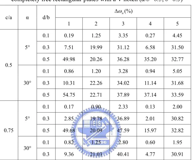
(32) cracked plate. Obviously, it is not suitable to characterize a V-notch in a plate only through the integration domain in the Ritz method as the notch angle or the notch depth becomes smaller. However, the corner functions satisfying the free edge boundary conditions of the V-notch can definitely realize the existence of a V-notch or a crack in the formulation for the Ritz method.. 3.4 Numerical Results To show the effects of a V-notch on the vibrations of plates, this section presents the frequency parameters and the mode shapes for the first five modes of rectangular plates with various aspect ratio a/b and having a V-notch with various notch angle α and notch depth d/b at various locations c/a. The mode shapes are described by their nodal patterns (lines of zero displacement during the vibration of a mode). Tables 3.8 to 3.10 show the results of frequency parameters for the first five modes of rectangular plates with different a/b (1.0, 2.0 and 0.5), α (5° and 30°), d/b (0, 0.1, 0.3 and 0.5) and c/a (0.5 and 0.75). Tables 3.11 to 3.13 show the relative reductions of the frequency parameters, which are defined as Δω n =. ω n ,intact − ω n ,V -notch × 100% , ω n ,intact. (3.14). where ωn,intact denotes the frequency of a intact plate, and ωn,V-notch denotes the frequency of a plate with a V-notch. It is interesting to observe how the frequency parameters change with 20.
(33) various α, d/b and c/a. Some interesting trends are found as follows: (1) The frequency parameters significantly decrease as the notch depth d/b increases for rectangular plates with different a/b mainly because of the reduction of the flexural stiffness. The decreasing frequencies relative to the frequencies of an intact plate are considerably different for different modes. (2) When d/b=0.5, the frequency parameters decrease if α changes from 5° to 30°. This trend is generally observed with few exceptions for d/b=0.1 and 0.3. (3) The frequency parameters for the first, second and fifth modes increase mostly as c/a changes from 0.5 to 0.75. The changes of the frequencies are more unpredictable for third and fourth modes. Since the nodal patterns of a square plate are different from those of other rectangular plates, they are discussed independently. Figures 3.2 and 3.3 show the nodal patterns for the first five modes of square plates (a/b=1.0) with different α, d/b and c/a, and the corresponding frequency parameters are given in the parenthesis. Before discussing the changes of the nodal patterns of a square plate for different α, d/b and c/a, it should be noticed that the nodal patterns of the fourth and fifth modes for an intact square plate shown in Fig. 3.2 and 3.3 are considerably different. Mathematically, the frequencies for these two modes are double roots in an eigenvalue problem, and any linear combination of the corresponding eigenfunctions is also a possible eigenfunction (as shown in Fig. 3.8). Consequently, the nodal patterns of the fourth and fifth modes shown in 21.
(34) these figures are correct, and there are infinite possible sets of mode shapes for the these two modes. The nodal patterns given in these figures are chosen because they resemble those for a square plate with a shallow V-notch and are often seen in published literature (i.e., Leissa, 1969). Some interesting trends for the changes of nodal patterns for a/b=1.0 with different α, d/b and c/a were found as follows: (1) For α fixed, the nodal patterns for d/b=0.1 looks very similar to those for d/b=0, respectively. However, if observing carefully, one can find some significant differences. A V-notch at c/a=0.5 destroys the symmetry about the horizontal axis, and the notch at c/a=0.75 further destroys the symmetry both axes. The crossing nodal lines for d/b=0 may separate when a V-notch exists (i.e., the second and fifth modes in Fig. 3.2). A straight nodal line for d/b=0 may be distorted when a V-notch exists (i.e., the diagonal nodal lines of the fourth and fifth modes in Fig. 3.3 and the horizontal nodal line of the second mode in Fig. 3.2). The curve veering and the distortion of the straight nodal lines would become more significant when α or d/b increases. (2) As d/b changes from 0.1 to 0.3, the changes of the nodal patterns become more significant, especially that the closed nodal line of the third mode is destroyed drastically. Note that modal order may exchange, for example, the nodal pattern of the fourth mode for the plate with α=30° and d/b=0.3 is similar to that of the fifth mode for the plate with α=30° and d/b=0.1 in Fig. 3.2. (3) As d/b changes from 0.3 to 0.5, the nodal patterns further change, 22.
(35) especially for the plate with c/a=0.75. Note that modal order may also exchange (i.e., the third and fourth modes in Fig. 3.2). (4) The changes of the nodal patterns for c/a=0.75 are more significant those for c/a=0.5 due to the destruction of the symmetry about the vertical axis cause by a V-notch at c/a=0.75. The crossing nodal lines of the first mode would separate as the V-notch is not at c/a=0.5. (5) The nodal patterns for α=5° look similar to those for α=30°, but the difference of those between α=5° and α=30° is more significant for the deeper V-notch. For example, the nodal patterns of the fifth mode for the plate with d/b=0.5 and c/a=0.75 are very different between α=5° and α=30°. Figures 3.4 to 3.7 show the nodal patterns for the first five modes of rectangular plates of a/b=2.0 and a/b=0.5 with different α, d/b and c/a. It is noticed that the intact plate for a/b=2.0 is the same as that for a/b=0.5. The V-notch is opening at the long edge for a/b=2.0, but that is opening at the short edge for a/b=0.5. It is also interesting to observe how the nodal patterns of rectangular plates with a/b=2.0 and a/b=0.5 change with different α, d/b and c/a, and these observations are given as follows: (1) As d/b changes from 0 to 0.1, the nodal patterns changes very slightly. Some differences similar to those for square plates can be found. When a V-notch exists, the crossing nodal lines for d/b=0 may separate (i.e., the second and third modes in Fig. 3.5 and the second and third modes in Fig. 3.7), and the straight nodal lines for d/b=0 may be distorted (i.e., the horizontal nodal line of the second mode in 23.
(36) Fig. 3.4 and the horizontal nodal line of the second and fourth modes in Fig. 3.6). (2) As d/b changes from 0.1 to 0.3, the curve veering and the distortion of the straight nodal lines become more significant. The nodal patterns still look similar between d/b=0.1 and d/b=0.3 for the plates with a/b=2.0, but they look very different for the plates with a/b=0.5. Note that modal order may also exchange for the plates with a/b=0.5 (i.e., the first and second modes in Fig. 3.6 and 3.7). (3) As d/b changes from 0.3 to 0.5, the nodal patterns further change, especially for the plates with a/b=0.5. Note that modal order may also exchange for the plates with a/b=2.0 (i.e., the third and fourth modes in Fig. 3.4 and the fifth mode in Fig. 3.4 and 3.5). (4) The changes of the nodal patterns for c/a=0.75 are more significant those for c/a=0.5 due to the destruction of the symmetry about vertical axis. The crossing nodal lines in the some modes would separate as the V-notch is not at c/a=0.5 (i.e., the second mode in Fig. 3.5 and the second and third modes in Fig.3.7). (5) As α changes from 5° to 30°, the curve veering and the distortion of the straight nodal lines become more significant. But the nodal patterns for α=5° and α=30° still look very similar with very slight difference. (6) The nodal patterns changes more violently when the V-notch is opening at short edge (a/b=0.5), especially for the fourth and fifth modes. 24.
(37) Chapter 4 Vibrations of Cantilevered Rectangular Plates This chapter investigates the vibrations of cantilevered rectangular plates with a V-notch as shown in Fig. 4.1. The same analysis procedure given in the previous chapter is used again here. This chapter also studies the effects of the configuration of a V-notch on the vibration behaviors of the plates under consideration.. 4.1 Admissible Functions The admissible functions used in the Ritz method have to satisfy the geometry boundary conditions of the problem under consideration. Accordingly, the admissible functions given in Eqs. (3.10) and (3.11) are modified as wp =. I +1 J −1. ∑ ∑a. i = 2 , 3 j = 0 ,1. wc (r , θ ) = x 2. ij. (4.1). xi y j ,. N. ∑ [a. n =1, 2. n. Re( wn (r , θ )) + a n Im(wn (r , θ ))] .. (4.2). The coordinate systems used in the problem under consideration are shown in Fig. 4.1. The relations between ( x, y ) and (r ,θ ) coordinates are the same as those used in a completely free plate, and are given in Eqs. (3.12) and (3.13).. 4.2 Convergence Study Through solving the generalized eigenvalue problem given in Eq. (3.6) by substituting the admissible functions given in Eqs. (4.1) and (4.2) into Eqs. (3.7) and (3.8), one can obtain the convergent upper-bound 25.
(38) solutions of the problem under consideration as the number of admissible functions is large enough. This section presents convergence studies for cantilevered square plates (a/b=1.0) with various notch angles (α=5° and 30°) and notch depths (d/b=0.1, 0.3, and 0.5). The V-notch is located at c/a=0.5. Poisson’s ratio υ is set to 0.3. To demonstrate the validity of the present method, this section also presents convergence for the plate with a straight crack (α=0°) parallel to the clamped edge and make a comparison with the results from previous investigation. The computation was carried out by using FORTRAN programming language with quad precision (34 significant digit accuracy) on a 64-bit computer. Table 4.1 shows the convergence of the frequency parameters for an intact square plate (no V-notch). Since there is no stress singularity existing, the admissible functions used in the formulation need not add any corner function. The numerical results of the frequency parameters were computed by polynomial functions, given in Eq. (4.2), with the number of terms (I×J) increasing from 3×3 to 10×10. The numerical results show excellent agreement with those by Leissa (1973), who used beam functions as admissible functions, and those by Rossi and Laura (1996), who used finite element method. The comparison demonstrates the validity of the computation for the part of the polynomial functions. Table 4.2 shows the convergence of the frequency parameters for a square plate with a shallow a V-notch (d/b=0.03) having large angle (α=170°). Although there are weak stress singularities existing at the vertex of the V-notch, the admissible polynomials still give good convergent results due to the completeness of polynomials. By adding 26.
(39) corner functions to the admissible functions, the convergence of the numerical solutions can be accelerated slightly. This case demonstrates the validity of the computation for using polynomials and corner functions as admissible functions. Tables 4.3 to 4.6 show the convergence of the frequency parameters for square plates having a V-notch with various notch angles (α=5° and 30°) and notch depths (d/b=0.1, 0.3 and 0.5). Since the V-notch is much sharper and deeper than that considered in Table 4.2, the corner functions are expected to show more significant effects on the convergence of the solutions due to the stronger stress singularities. In these cases under study, the admissible polynomials used alone give solutions with very slow convergence, especially for the case with a sharper (α=5°) or deeper (d/b=0.5) notch. However, through supplementing the admissible functions with corner functions, the convergence of the solutions can be accelerated significantly. Observing the results of Table 4.3, one finds that adding the corner functions into the admissible polynomials may yield ill-conditioned matrices at the number of admissible functions not very large (i.e., 8×8+2×8, 7×7+2×8). If the admissible polynomials are used alone in the formulation, the ill-conditioning occurs when the number of polynomials (I×J) exceeds 12×12. The numerical solutions cannot be convergent to the exact ones by using polynomial functions only before the ill-conditioning occurs. Nevertheless, supplementing the admissible functions with corner functions can give the convergent solutions with high accuracy (at least 3 significant digit convergence) before the 27.
(40) ill-conditioning occurs. Comparing the results of Table 4.3 with those of Tables 4.4 and 4.5, one can find that to obtain the convergent solutions for square plates with a deeper V-notch needs to add more corner functions into the admissible functions. Comparing the results of Tables 4.4 and 4.6, one can find that more corner functions may not be needed to obtain convergent solutions as α changes from 30° to 5°. Note that, without the supplement of corner functions, one may overestimate the solutions of these cases. Table 4.7 shows the convergence of the frequency parameters for a square plate having a V-notch with α=0° and d/b=0.25, which can be considered as a straight crack. As expected, the solution obtained by using only polynomial functions is the same as that of an intact plate due to the same integral domain. The correct solutions of a cracked plate should be less than that of an intact plate, because the crack causes damage to the flexural stiffness of a plate. Through supplementing the admissible functions with corner functions, the frequencies can decrease efficiently due to the recognition of the existence of a crack in the Ritz method. Ma and Huang (2001) used the AFESPI experimental method to investigate the vibrations of a cantilevered square plate with a crack, and also simulate those by the commercial finite element package ABAQUS. This experiment used a full field, non-contact technique, electronic speckle pattern interferometry, for vibration measurement. The eight-node shell elements S8R5 were used in ABAQUS. Comparing the numerical results obtained from the present method to those by ABAQUS, the 28.
(41) formers are little greater than the latters. This trend is expected mainly because the elements S8R5 were based on the first-order shear deformation plate theory that has less constraints than the classical plate theory. Comparing the present numerical results to the experimental results, the present ones are all greater than the experimental ones. The main reason is believed that the clamped boundary condition of the plate for the experiment is not ideally rigid. The good agreement between these results demonstrates the validity of the present method.. 4.3 Numerical Results Tables 4.8 to 4.10 show the results of frequency parameters for the first five modes of rectangular plates with different a/b (1.0, 2.0 and 0.5), α (5° and 30°), d/b (0, 0.1, 0.3 and 0.5) and c/a (0.5 and 0.75), and tables 4.11 to 4.13 show the relative reductions of the frequency parameters. It is interesting to observe how the frequency parameters change with various α, d/b and c/a. Some interesting findings were observed, and are given as follows: (1) The frequency parameters significantly decrease with the increasing notch depth d/b for rectangular plates with different a/b mainly because of the reduction of the flexural stiffness. (2) Generally, the frequency parameters decrease as α changes from 5° to 30° for deeper V-notches. Very few exceptions are found for d/b=0.1 and 0.3. (3) The frequency parameters for the first and second modes increase as 29.
(42) c/a changes from 0.5 to 0.75 for rectangular plates with different a/b. For such modes, the reduction of the flexural stiffness would increase as the V-notch is near to the clamped edge. Figures 4.2 to 4.7 show the nodal patterns for the first five modes of square plates with different a/b, α, d/b and c/a, and the corresponding frequency parameters are given in the parenthesis. It is also interesting to observe the changes of nodal patterns with different α, d/b and c/a. These interesting findings are given as follows: (1) For intact plates (d/b=0), the nodal patterns of the fourth and fifth modes exchange as a/b changes from 1.0 to 2.0. As a/b changes from 1.0 to 0.5, the nodal patterns of the third to fifth modes for the plate with a/b=1.0 are very different from those for a/b=0.5. (2) For α fixed, the first five nodal patterns for d/b=0.1 looks very similar to those for d/b=0, except that the crossing nodal lines for d/b=0 would separate clearly (i.e., the fifth mode in Fig. 4.2 and the fourth mode in Fig. 4.4). Furthermore, if observing carefully, one can find some slight differences existing in the nodal patterns for intact plats and V-notched plates. Since a V-notch destroys the symmetry about horizontal axis, the mode shapes are no longer symmetric about horizontal axis. The horizontal nodal lines for d/b=0 is distorted when a V-notch exists (i.e., the second mode in Fig. 4.2). (3) As d/b changes from 0.1 to 0.3, the changes of the nodal patterns become clearer, especially for third, fourth and fifth modes for the plate with a/b=0.5. Note that modal order may exchange (i.e., the 30.
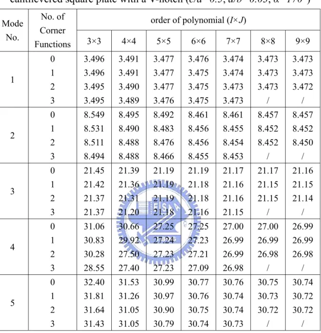
(43) fourth and fifth modes in Fig. 4.6) (4) As d/b changes from 0.3 to 0.5, the nodal patterns further change, especially for the plates with a/b=0.5. Note that an additional nodal line would appear in the nodal patterns of the first mode for the plates with a/b=0.5. (5) Generally, the changes of the nodal patterns are more significant for the V-notch at c/a=0.5. The difference of the nodal patterns between c/a=0.5 and c/a=0.75 are very slight for d/b=0.1 but clearer for d/b=0.3 and 0.5. (6) The nodal patterns for α=5° look similar to those for α=30°. The difference of nodal patterns between α=5° and α=30° are more significant as d/b increases.. 31.
(44) Chapter 5 Concluding Remarks In the previous chapters, vibration behaviors of completely free and cantilevered rectangular plates with an edge V-notch have been determined via the present method. Some conclusions are drawn from the foregoing studies: (1) The corner functions exactly satisfy the free boundary conditions along a V-notch and appropriately describe the stress singularity behaviors around the vertex of a V-notch. It has been demonstrated that the convergence of the numerical solutions can be accelerated by supplementing the admissible functions in the Ritz method with the corner functions. (2) Matrix ill-conditioning occurs when the total number of admissible functions used is too large. Through the supplements of corner functions, one can obtain the convergent solutions with high accuracy (4 significant digit convergence) before the ill-conditioning occurs. (3) It has been shown that poor convergence is obtained by using polynomial functions only when plates with a sharp V-notch. As the V-notch becomes deeper, it needs more number of corner functions to obtain accurate solutions. (4) It has been shown that a shallow V-notch has only a small effect on the vibration behaviors of a V-notch plate. As the V-notch is deeper, frequencies significantly decrease mainly because of the reduction of the flexural stiffness, and the nodal patterns changes more violently. The 32.
(45) curve veering and the distortion of the straight nodal lines may occur due to the destruction of the symmetry when a V-notch exists. Sometimes, the modal order may exchange as the notch depth varies. The thesis accurately determines vibration frequencies and nodal patterns of V-notched rectangular plates via the present method. These present results serve not only to improve the understanding the vibration behavior of a V-notched plate, but also as benchmark data against those from other numerical methods or experiments. The analysis methodology used here can be extended to other thin plate problems with stress singularities, such as a plate with a cut-out where more than one corners having stress singularities exist.. 33.
(46) References Aggarwala, B. D. and Ariel, P. D. (1981) “Vibration and bending of a cracked plate”, Rozprawy Inzynierskie, 29(2), pp. 295-310. Filipich, C. P. and Rosales, M. B. (2000) “Arbitrary precision frequencies of a free rectangular thin plate”, Journal of Sound and Vibration, 230(3), pp. 521-539. Hirano, Y. and Okazaki, K. (1980) “Vibration of cracked rectangular plates”, Bulletin of the Japan Society of Mechanical Engineers, 23(179), pp. 732-740. Huang, C. S. (1991) Singularities in plate vibration problems, Ph. D. dissertation, The Ohio State University, Columbus, Ohio. Khadem, S. E. and Rezaee, M. (2000) “Introduction of modified comparison functions for vibration analysis of a rectangular cracked plate”, Journal of Sound and Vibration, 236(2), pp. 245-258. Krawczuk, M (1993) “Natural vibrations of rectangular plates with a through crack”, Archive of Applied Mechanics, 63(7), pp. 491-504. Leissa, A. W., McGee, O. G. and Huang, C. S. (1993) “Vibrations of Circular Plates Having V-notches or Sharp Radial Cracks”, Journal of Sound and Vibration, 161(2), pp. 227-239. Leissa, A. W., McGee, O. G. and Huang, C. S. (1993) “Vibrations of Sectorial Plates Having Corner Stress Singularities”, Journal of Applied Mechanics, 60, pp. 136-140. 34.
(47) Leissa, A. W. (1973) “The free vibration of rectangular plates”, Journal of Sound and Vibration, 31(3), pp. 257-293. Leissa, A. W. (1969) Vibration of plates, NASA SP-160. Liew, K. M., Hung, K. C. and Lim, M. K. (1994) “A solution method for analysis of cracked plates under vibration”, Engineering Fracture Mechanics, 48(3), pp. 393-404. Lynn, P. P. and Kumbasar, N. (1967) “Free vibrations of thin rectangular plates having narrow cracks with simply supported edges”, Developments in Mechanics, 4, Proc. 10th Midwestern Mechanics Conference, Colorado State University, Fort Collins, Colorado, August 21-23, pp. 911-928. Ma, C. C. and Huang, C. H. (2001) “Experimental and numerical analysis of vibrating cracked plates at resonant frequencies”, Experimental Mechanics, 41(1), pp. 8-18. Neku, K. (1982) “Free vibration of a simply-supported rectangular plate with a straight through-notch”, Bulletin of the Japan Society of Mechanical Engineers, 25(199), pp. 16-23. Qian, G. L., Gu, S. N. and Jiang, J. S. (1991) “A finite element model of cracked plates and application to vibration problems”, Computers and Structures, 39(5), pp. 483-487. Rossi, R. E. and Laura, P. A. A. (1996) “Symmetric and antisymmetric normal modes of a cantilever rectangular plate: effect of Poisson’s ratio and a concentrated mass”, Journal of Sound and Vibration, 195(1), pp. 35.
(48) 142-148. Solecki, R. (1983) “Bending vibration of a simply supported rectangular plate with a crack parallel to one edge”, Engineering Fracture Mechanics, 18(6), pp. 1111-1118. Stahl, B. and Keer, L. M. (1972) “Vibration and Stability of cracked rectangular plates”, International Journal of Solids and Structures, 8(1), pp. 69-91. Timoshenko, S. and Woinowsky-Krieger, S. (1959), Theory of plates and shells, 2nd edition, McGraw-Hill. Williams, M. L. (1952) “Surface Stress Singularities Resulting from Various Boundary Conditions in Angular Corners of Plates under Bending”, Proceedings of the First U.S. National Congress of Applied Mechanics, pp.325-329. Yuan, J. and Dickinson, S. M. (1992) “The flexural vibration of rectangular plate systems approached by using artificial springs in the Rayleigh-Ritz method”, Journal of Sound and Vibration, 159(1), pp. 39-55. 36.
(49) Table 3.1 Convergence of frequency parameters ωa 2 ρh / D for a completely free square plate order of polynomial (I×J). Mode No. 3×3. 4×4. 5×5. 6×6. 7×7. 8×8. 9×9. Leissa (1973). Filipich and Rosales (2000). 10×10. 1. 14.20 13.66 13.66 13.47 13.47 13.47 13.47. 13.47. 13.49. 13.47. 2. 22.45 22.45 19.73 19.73 19.60 19.60 19.60. 19.60. 19.79. 19.61. 3. 30.59 30.59 24.54 24.54 24.27 24.27 24.27. 24.27. 24.43. 24.28. 4. 41.57 39.23 35.61 35.29 34.81 34.80 34.80. 34.80. 35.02. 34.82. 5. 41.57 39.23 35.61 35.29 34.81 34.80 34.80. 34.80. 35.02. 38.82. 37.
(50) Table 3.2 Convergence of frequency parameters ωa 2 ρh / D for a completely free square plate with a V-notch (c/a=0.5, d/b=0.03, α=170°) Mode No.. No. of Corner Functions. 3×3. 4×4. 5×5. 6×6. 7×7. 8×8. 9×9. 1. 0 1 2 3. 14.22 14.22 14.22 14.15. 13.67 13.66 13.65 13.65. 13.67 13.66 13.65 13.59. 13.49 13.48 13.48 13.48. 13.49 13.48 13.48 13.47. 13.48 13.48 13.47 13.47. 13.48 13.48 13.47 13.47. 2. 0 1 2 3. 22.08 21.44 21.41 19.77. 22.08 21.40 20.34 19.63. 19.43 19.42 19.42 19.42. 19.43 19.42 19.42 19.42. 19.31 19.30 19.30 19.30. 19.31 19.30 19.30 19.30. 19.31 19.30 19.30 19.29. 3. 0 1 2 3. 30.62 29.43 29.42 29.35. 30.62 29.38 27.04 25.65. 24.58 24.56 24.56 24.55. 24.58 24.56 24.55 24.52. 24.32 24.32 24.32 24.31. 24.32 24.32 24.32 24.31. 24.32 24.32 24.32 24.31. 4. 0 1 2 3. 41.40 40.04 39.37 38.93. 38.97 37.90 37.90 35.84. 35.48 35.37 35.36 35.27. 35.14 35.05 35.03 35.00. 34.71 34.69 34.69 34.66. 34.70 34.68 34.68 34.65. 34.69 34.67 34.67 34.64. 5. 0 1 2 3. 41.71 41.69 40.64 40.64. 39.40 39.05 38.72 37.21. 35.66 35.61 35.58 35.57. 35.35 35.31 35.28 35.17. 34.85 34.83 34.82 34.80. 34.84 34.81 34.80 34.79. 34.84 34.81 34.80 34.78. order of polynomial (I×J). 38.
(51) Table 3.3 Convergence of frequency parameters ωa 2 ρh / D for a completely free square plate with a V-notch (c/a=0.5, d/b=0.1, α=30°) Mode No.. No. of Corner Functions. 4×4. 5×5. 6×6. 7×7. 8×8. 9×9. 10×10. 1. 0 3 5 8 10. 13.68 13.50 13.48 13.34 13.32. 13.68 13.50 13.42 13.33 13.32. 13.49 13.32 13.31 13.31 13.31. 13.49 13.32 13.31 13.31 /. 13.49 13.31 13.31 / /. 13.49 13.31 13.31 / /. 13.49 13.31 13.31 / /. 2. 0 3 5 8 10. 22.35 20.68 19.72 19.44 19.40. 19.65 19.41 19.40 19.35 19.31. 19.65 19.41 19.39 19.32 19.31. 19.52 19.31 19.31 19.31 /. 19.52 19.31 19.31 / /. 19.52 19.31 19.31 / /. 19.52 19.31 19.31 / /. 3. 0 3 5 8 10. 30.62 28.28 24.49 24.37 24.37. 24.57 24.36 24.29 24.20 24.10. 24.57 24.36 24.29 24.10 24.10. 24.31 24.10 24.09 24.09 /. 24.31 24.10 24.09 / /. 24.31 24.10 24.09 / /. 24.31 24.10 24.09 / /. 4. 0 3 5 8 10. 39.11 36.40 35.27 34.73 34.67. 35.53 34.80 34.65 34.43 34.17. 35.20 34.45 34.38 34.25 34.11. 34.74 34.08 34.07 34.07 /. 34.74 34.07 34.07 / /. 34.73 34.07 34.07 / /. 34.73 34.07 34.07 / /. 5. 0 3 5 8 10. 39.35 37.50 36.00 34.91 34.70. 35.68 34.96 34.92 34.88 34.57. 35.37 34.70 34.52 34.31 34.22. 34.88 34.23 34.23 34.22 /. 34.87 34.22 34.22 / /. 34.87 34.22 34.22 / /. 34.87 34.22 34.22 / /. order of polynomial (I×J). Note:“/”:no result due to matrix ill-conditioning. 39.
(52) Table 3.4 Convergence of frequency parameters ωa 2 ρh / D for a completely free square plate with a V-notch (c/a=0.5, d/b=0.3, α=30°) Mode No.. No. of Corner Functions. 3×3. 4×4. 5×5. 6×6. 7×7. 8×8. 1. 0 3 5 10 15. 14.36 11.82 11.75 11.61 11.60. 13.82 11.67 11.67 11.57 11.56. 13.82 11.67 11.64 11.56 11.56. 13.62 11.57 11.56 11.56 11.56. 13.62 11.57 11.56 11.56 11.56. 13.61 11.57 11.56 11.56 11.56. 2. 0 3 5 10 15. 22.06 18.16 17.64 17.15 17.13. 22.05 18.13 17.38 17.14 17.12. 19.41 17.17 17.15 17.09 17.09. 19.41 17.15 17.14 17.09 17.09. 19.29 17.09 17.09 17.08 17.08. 19.29 17.09 17.09 17.08 17.08. 3. 0 3 5 10 15. 30.85 26.24 26.21 23.31 23.23. 30.84 26.15 23.65 23.16 23.11. 24.78 23.19 23.17 22.97 22.95. 24.78 23.19 23.16 22.95 22.95. 24.54 22.95 22.95 22.94 22.94. 24.54 22.95 22.95 22.94 22.94. 4. 0 3 5 10 15. 40.96 33.36 29.41 28.20 27.92. 38.64 28.71 28.14 27.71 27.66. 35.25 28.05 27.92 27.67 27.55. 34.91 27.75 27.67 27.53 27.53. 34.57 27.62 27.56 27.53 27.53. 34.56 27.57 27.53 27.52 27.52. 5. 0 3 5 10 15. 42.13 36.63 34.16 32.18 31.83. 39.98 35.04 33.48 32.00 31.67. 36.15 32.04 32.01 31.58 31.45. 35.88 31.82 31.77 31.49 31.44. 35.34 31.45 31.45 31.44 31.43. 35.30 31.45 31.44 31.43 31.43. order of polynomial (I×J). 40.
(53) Table 3.5 Convergence of frequency parameters ωa 2 ρh / D for a completely free square plate with a V-notch (c/a=0.5, d/b=0.5, α=30°) Mode No.. No. of Corner Functions. 3×3. 4×4. 5×5. 6×6. 7×7. 8×8. 1. 0 3 5 10 15. 14.60 7.974 7.948 7.890 7.883. 14.07 7.915 7.906 7.852 7.850. 14.06 7.902 7.873 7.849 7.847. 13.86 7.867 7.850 7.845 7.845. 13.86 7.865 7.849 7.845 7.844. 13.85 7.863 7.848 7.844 7.843. 2. 0 3 5 10 15. 22.06 14.45 14.05 13.89 13.88. 22.04 14.38 13.99 13.87 13.85. 19.48 13.89 13.87 13.84 13.83. 19.48 13.88 13.86 13.84 13.83. 19.36 13.83 13.83 13.82 13.82. 19.36 13.83 13.83 13.82 13.82. 3. 0 3 5 10 15. 30.93 22.88 22.02 21.56 21.44. 30.89 21.75 21.59 21.30 21.28. 25.03 21.63 21.50 21.28 21.25. 25.02 21.35 21.29 21.22 21.21. 24.78 21.32 21.26 21.22 21.21. 24.78 21.25 21.22 21.21 21.21. 4. 0 3 5 10 15. 40.48 24.00 23.68 22.13 22.09. 38.38 23.98 22.94 22.01 21.98. 35.22 22.05 22.04 21.91 21.89. 34.89 22.05 22.04 21.89 21.88. 34.63 21.89 21.88 21.88 21.88. 34.62 21.89 21.88 21.88 21.88. 5. 0 3 5 10 15. 42.70 35.54 34.51 31.91 31.61. 40.64 34.13 33.35 31.47 31.16. 36.73 31.60 31.51 31.13 30.94. 36.49 31.37 31.27 31.03 30.93. 35.92 31.02 30.93 30.93 30.92. 35.84 31.02 30.93 30.92 30.92. order of polynomial (I×J). 41.
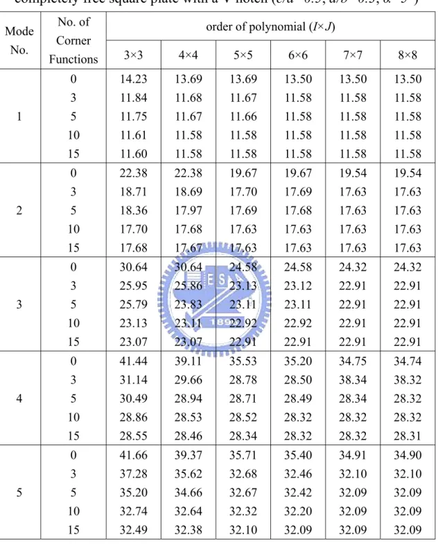
(54) Table 3.6 Convergence of frequency parameters ωa 2 ρh / D for a completely free square plate with a V-notch (c/a=0.5, d/b=0.3, α=5°) Mode No.. No. of Corner Functions. 3×3. 4×4. 5×5. 6×6. 7×7. 8×8. 1. 0 3 5 10 15. 14.23 11.84 11.75 11.61 11.60. 13.69 11.68 11.67 11.58 11.58. 13.69 11.67 11.66 11.58 11.58. 13.50 11.58 11.58 11.58 11.58. 13.50 11.58 11.58 11.58 11.58. 13.50 11.58 11.58 11.58 11.58. 2. 0 3 5 10 15. 22.38 18.71 18.36 17.70 17.68. 22.38 18.69 17.97 17.68 17.67. 19.67 17.70 17.69 17.63 17.63. 19.67 17.69 17.68 17.63 17.63. 19.54 17.63 17.63 17.63 17.63. 19.54 17.63 17.63 17.63 17.63. 3. 0 3 5 10 15. 30.64 25.95 25.79 23.13 23.07. 30.64 25.86 23.83 23.11 23.07. 24.58 23.13 23.11 22.92 22.91. 24.58 23.12 23.11 22.92 22.91. 24.32 22.91 22.91 22.91 22.91. 24.32 22.91 22.91 22.91 22.91. 4. 0 3 5 10 15. 41.44 31.14 30.49 28.86 28.55. 39.11 29.66 28.94 28.53 28.46. 35.53 28.78 28.71 28.52 28.34. 35.20 28.50 28.49 28.32 28.32. 34.75 38.34 28.34 28.32 28.32. 34.74 38.32 28.32 28.32 28.31. 5. 0 3 5 10 15. 41.66 37.28 35.20 32.74 32.49. 39.37 35.62 34.66 32.64 32.38. 35.71 32.68 32.67 32.32 32.10. 35.40 32.46 32.42 32.20 32.09. 34.91 32.10 32.09 32.09 32.09. 34.90 32.10 32.09 32.09 32.09. order of polynomial (I×J). 42.
(55) Table 3.7 Convergence of frequency parameters ωa 2 ρh / D for a completely free square plate with a V-notch (c/a=0.5, d/b=0.3, α=0°) Mode No.. No. of Corner Functions. 4×4. 5×5. 6×6. 7×7. 8×8. 9×9. 10×10. 1. 0 3 5. 13.66 11.80 11.68. 13.66 11.79 11.66. 13.47 11.65 11.63. 13.47 11.65 11.63. 13.47 11.64 11.63. 13.47 11.64 11.63. 13.47 11.63 11.62. 2. 0 3 5. 22.45 18.49 18.35. 19.73 17.86 17.80. 19.73 17.86 17.78. 19.60 17.78 17.78. 19.60 17.78 17.78. 19.60 17.77 17.77. 19.60 17.77 17.77. 3. 0 3 5. 30.59 26.03 25.43. 24.54 23.10 23.09. 24.54 23.10 23.09. 24.27 22.89 22.89. 24.27 22.89 22.89. 24.27 22.89 22.89. 24.27 22.89 22.89. 4. 0 3 5. 39.23 30.37 30.16. 35.61 29.22 29.09. 35.29 28.90 28.76. 34.81 28.74 28.65. 34.80 28.66 28.63. 34.80 28.66 28.63. 34.80 28.64 28.62. 5. 0 3 5. 39.23 35.07 32.95. 35.61 32.90 32.84. 35.29 32.67 32.56. 34.81 32.31 32.30. 34.80 32.30 32.30. 34.80 32.30 32.30. 34.80 32.30 32.30. order of polynomial (I×J). 43.
(56) Table 3.8 Frequency parameters ωa 2 ρh / D for completely free rectangular plates with a V-notch (a/b=1.0, υ=0.3) c/a. α. 5° 0.5 30°. 5° 0.75 30°. ωa 2 ρ h / D. d/b 1. 2. 3. 4. 5. 0*. 13.47. 19.60. 24.27. 34.80. 34.80. 0.1. 13.31. 19.40. 24.08. 34.20. 34.21. 0.3. 11.58. 17.63. 22.91. 28.31. 32.09. 0.5. 8.178. 14.48. 21.97. 22.54. 31.55. 0.1. 13.31. 19.31. 24.09. 34.07. 34.22. 0.3. 11.56. 17.08. 22.94. 27.52. 31.43. 0.5. 7.843. 13.82. 21.21. 21.88. 30.92. 0.1. 13.36. 19.52. 24.20. 34.19. 34.64. 0.3. 12.07. 18.38. 22.80. 27.61. 33.75. 0.5. 8.515. 15.12. 20.96. 24.82. 32.87. 0.1. 13.33. 19.48. 24.18. 34.17. 34.56. 0.3. 11.86. 18.16. 22.54. 27.05. 33.20. 0.5. 7.961. 14.60. 20.57. 24.37. 32.27. Note:*:No V-notch. 44.
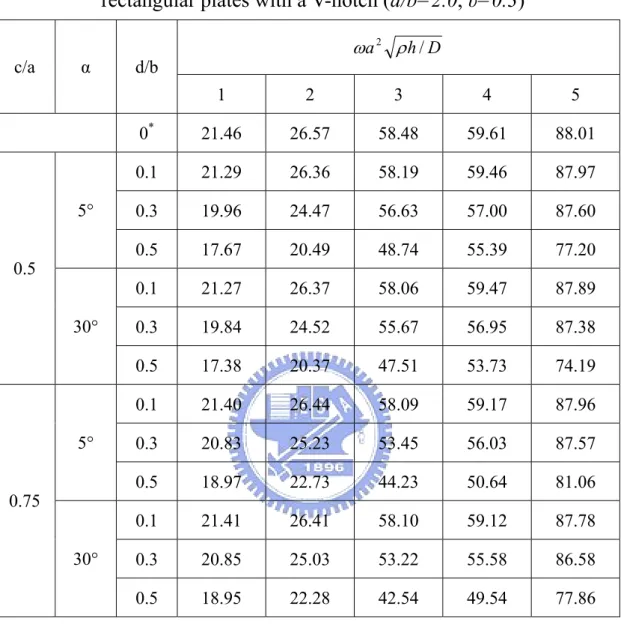
(57) Table 3.9 Frequency parameters ωa 2 ρh / D for completely free rectangular plates with a V-notch (a/b=2.0, υ=0.3) c/a. α. 5° 0.5 30°. 5° 0.75 30°. ωa 2 ρ h / D. d/b 1. 2. 3. 4. 5. 0*. 21.46. 26.57. 58.48. 59.61. 88.01. 0.1. 21.29. 26.36. 58.19. 59.46. 87.97. 0.3. 19.96. 24.47. 56.63. 57.00. 87.60. 0.5. 17.67. 20.49. 48.74. 55.39. 77.20. 0.1. 21.27. 26.37. 58.06. 59.47. 87.89. 0.3. 19.84. 24.52. 55.67. 56.95. 87.38. 0.5. 17.38. 20.37. 47.51. 53.73. 74.19. 0.1. 21.40. 26.44. 58.09. 59.17. 87.96. 0.3. 20.83. 25.23. 53.45. 56.03. 87.57. 0.5. 18.97. 22.73. 44.23. 50.64. 81.06. 0.1. 21.41. 26.41. 58.10. 59.12. 87.78. 0.3. 20.85. 25.03. 53.22. 55.58. 86.58. 0.5. 18.95. 22.28. 42.54. 49.54. 77.86. Note:*:No V-notch. 45.
(58) Table 3.10 Frequency parameters ωa 2 ρh / D for completely free rectangular plates with a V-notch (a/b=0.5, υ=0.3) c/a. α. 5° 0.5 30°. 5° 0.75 30°. ωa 2 ρ h / D. d/b 1. 2. 3. 4. 5. 0*. 5.366. 6.644. 14.62. 14.90. 22.00. 0.1. 5.356. 6.561. 14.13. 14.86. 21.02. 0.3. 4.963. 5.316. 10.07. 13.92. 15.07. 0.5. 2.684. 5.298. 9.316. 9.655. 14.79. 0.1. 5.320. 6.564. 14.14. 14.76. 20.89. 0.3. 4.813. 5.165. 9.647. 13.24. 15.03. 0.5. 2.428. 5.135. 9.081. 9.366. 14.61. 0.1. 5.357. 6.584. 14.28. 14.88. 21.56. 0.3. 5.213. 5.330. 9.226. 14.60. 15.22. 0.5. 2.700. 5.309. 7.662. 12.52. 14.78. 0.1. 5.322. 6.561. 14.21. 14.81. 21.57. 0.3. 4.864. 5.247. 8.712. 14.19. 15.20. Note:*:No V-notch. 46.
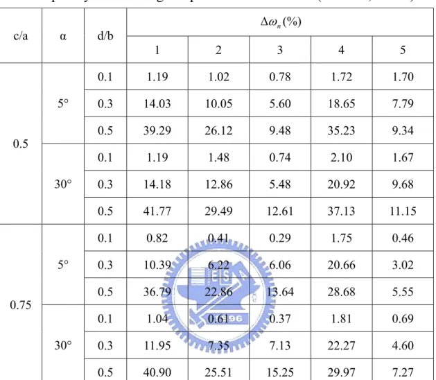
(59) Table 3.11 Relative reductions of the frequency parameters Δωn for completely free rectangular plates with a V-notch (a/b=1.0, υ=0.3) c/a. α. 5° 0.5 30°. 5° 0.75 30°. Δωn (%). d/b 1. 2. 3. 4. 5. 0.1. 1.19. 1.02. 0.78. 1.72. 1.70. 0.3. 14.03. 10.05. 5.60. 18.65. 7.79. 0.5. 39.29. 26.12. 9.48. 35.23. 9.34. 0.1. 1.19. 1.48. 0.74. 2.10. 1.67. 0.3. 14.18. 12.86. 5.48. 20.92. 9.68. 0.5. 41.77. 29.49. 12.61. 37.13. 11.15. 0.1. 0.82. 0.41. 0.29. 1.75. 0.46. 0.3. 10.39. 6.22. 6.06. 20.66. 3.02. 0.5. 36.79. 22.86. 13.64. 28.68. 5.55. 0.1. 1.04. 0.61. 0.37. 1.81. 0.69. 0.3. 11.95. 7.35. 7.13. 22.27. 4.60. 0.5. 40.90. 25.51. 15.25. 29.97. 7.27. 47.
數據
+7

相關文件
However, there exist functions of bounded variation that are not continuously differentiable.... However, there exist bounded functions that are not of
Population: the form of the distribution is assumed known, but the parameter(s) which determines the distribution is unknown.. Sample: Draw a set of random sample from the
For example, Ko, Chen and Yang [22] proposed two kinds of neural networks with different SOCCP functions for solving the second-order cone program; Sun, Chen and Ko [29] gave two
In this paper, we build a new class of neural networks based on the smoothing method for NCP introduced by Haddou and Maheux [18] using some family F of smoothing functions.
Chen, The semismooth-related properties of a merit function and a descent method for the nonlinear complementarity problem, Journal of Global Optimization, vol.. Soares, A new
In summary, the main contribution of this paper is to propose a new family of smoothing functions and correct a flaw in an algorithm studied in [13], which is used to guarantee
In this paper, we extend this class of merit functions to the second-order cone complementarity problem (SOCCP) and show analogous properties as in NCP and SDCP cases.. In addition,
Proof. The proof is complete.. Similar to matrix monotone and matrix convex functions, the converse of Proposition 6.1 does not hold. 2.5], we know that a continuous function f
