多天線傳送系統干擾抑制及路徑衰減補償之可適性封包檢測

國 立 交 通 大 學

資訊科學與工程研究所

碩

士

論

文

多天線傳送系統干擾抑制

及路徑衰減補償

之可適性封包檢測

Adaptive Packet Acquisition

with Interference and Time-Variant

Path –Loss in MIMO-OFDM Systems

研 究 生 : 呂理聖

指導教授 : 許騰尹 教授

多天線傳送系統干擾抑制及路徑衰減補償

之可適性封包檢測

Adaptive Packet Acquisition with Interference

and Time-Variant Path-Loss in MIMO OFDM Systems

研 究 生：呂理聖

Student : Li-Sheng Lu

指導教授：許騰尹

Advisor : Terng-Yin Hsu

國 立 交 通 大 學

資訊科學與工程研究所

碩 士 論 文

A Thesis

Submitted to Department of Computer Science and Information Engineering College of Electrical Engineering and Computer Science

National Chiao Tung University in partial Fulfillment of the Requirements

for the Degree of Master

in

Computer Science and Information Engineering July 2006

Hsinchu, Taiwan, Republic of China

多天線傳送系統干擾抑制

及路徑衰減補償

之可適性封包檢測

學生：呂理聖 指導教授：許騰尹 博士

國立交通大學

資訊學院 資訊工程學系碩士班

摘要

在現代無線通訊系統中，多輸入輸出系統被廣泛的使用。對於多輸出輸入系統 我們將要面對一些問題，首先我們注意的是準確控制接收到的能量。因為接收到的 能量會被類比轉數位電路斬截，假如我們自動增益控制電路沒控制好，訊號可能會 失真或太小以至於無法偵測。我們要面對的第二個問題是封包到達與否。因為有兩 條以上的天線，我們控制自動增益控制電路去抵抗路徑衰減，且我們使用全部天線 的欄位結構來判定封包到達。還有一些雜訊干擾我們封包偵測，如臨接頻道干擾。 倘若我們沒有任何演算法去抵抗它，我們的封包偵測演算法將無法工作。

Adaptive Packet Acquisition with

Interference and Time-Variant Path-Loss

in MIMO OFDM Systems

Student:

Li-Sheng

Lu

Advisor:

Dr.

Terng-Yin

Hsu

Department of Computer Science and Information Engineering,

National Chiao Tung University

Abstract

MIMO system are widely used in modern wireless communications systems. In MIMO system, there are some problems we should face. The first problem we encounter is that precisely control the power of our received signals. Because the received signals will be truncated by ADC, if our AGC control isn’t good enough, signals will be distortion or will be too small to detect. The second problem we encounter is how to determine packet coming or not. Because there are two or more antennas in MIMO system, we control the AGC to resist the path loss, and we can use the preamble structure of all antennas to decision the packet coming. Last there are some noise infects our packet detection, such as adjacent channel interference (ACI). If there are not any algorithms to resist it, the packet detection will be always failed.

Table of Contents

page

Chapter 1 Introduction………...1

Chapter 2 System Model of MIMO-OFDM……...…...2

Chapter 3 Path Loss Model and Interference Model..……..…………...………5

Chapter 4 Timing Synchronization for MIMO system………10

Chapter 5 Matlab Simulation...……...…….………..19

Chapter 6 System Architecture…..………...23

Chapter 7 Conclusion and Future Work...…………...29

List of Figures

p a g e

Figure 2.1 MIMO Basic Architecture………..……...……….…….….2

Figure 2.2 Alamouti STBC（Space Time Block Code）...………..……….…….……3

Figure 2.3 MIMO Basic Transmitter...………..………..……….…….…3

Figure 2.4 MIMO Basic Receiver……...………..………..……….…….…3

Figure 2.5 System Channel Model…………...………...……….…4

Figure 3.1 The Received Signal without Path Loss………...……….……….5

Figure 3.2 Path Loss Modeling………..………...……….……....6

Figure 3.3 The Received Signal with Path Loss………...……….…….6

Figure 3.4 Imperfect Spectrum Mask……….………….7

Figure 3.5 Interference Modeling………....……….…..…….8

Figure 3.6 The Signal with Interference before ADC…………...……….9

Figure 3.7 The Signal with Interference after ADC……..……….………….9

Figure 4.1 Real Part of 1st Antenna HT-LTF2 after Truncated…...………..……14

Figure 4.2 Red: Compensation Real Part of 1st HT-LTF2………16

Figure 4.3 Adaptive Threshold Decision………...……....……17

Figure 4.4 Average Pilot Amplitude of 20 Symbols without AGC Tracking…...……17

Figure 4.5 Average Pilot Amplitude of 20 Symbols with AGC Tracking….…….……18

Figure 4.6 Timing Synchronization of Our system Block…….………..…18

Figure 5.1 PER vs SNR, MCS13, TGnD, SIR 10db, path loss vibrates -3db to +3db...20

Figure 5.2 PER vs SNR, MCS 13, TGnD, SIR 10db, IQ mismatch and FDI effect worst case, path loss vibrates -3db to +3db……….20

Figure 5.3 PER vs SNR, MCS13, TGnE, SIR 10db, path loss vibrates -3db to +3db…...21

Figure 5.4 PER vs SNR, MCS 13, TGnE, SIR 10db, IQ mismatch and FDI effect worst case, path loss vibrates -3db to +3db……….22

Figure 6.1 Architecture of MIMO packet detection…...……...………...24

Figure 6.2 the Architecture of Noise Control……….25

Figure 6.3 the Architecture of Interference Truncated………...25

Figure 6.4 the Architecture of Packet Detection………...…….26

Figure 6.5 the Architecture of Boundary Decision………...………….26

Figure 6.6 the Architecture of Time Domain Channel Response……….………….27

Chapter 1

Introduction

In MIMO system, there are some problems we should face. The first problem we encounter is that precisely control the power of our received signals. Because the received signals will be truncated by ADC, if our AGC control isn’t good enough, signals will be distortion or will be too small to detect. The second problem we encounter is how to determine packet is coming or not. Because there are two or more antennas in MIMO system, we control the AGC to resist the path loss, and we can use the preamble structure of all antennas to decision the packet coming. Last there are some noise infects our packet detection, such as adjacent channel interference (ACI). If there are not any algorithms to resist it, the packet detection will be always failed.

This thesis is organized as follows. Chapter 2 introduces the basics of MIMO systems and wireless channel model. Chapter 3 introduces the interference modeling and path loss modeling. Chapter 4 presents the timing synchronization for MIMO system, it includes AGC control, packet detection, AGC tracking, interference compensation. Chapter 5 discusses the Matlab simulation results under different conditions. Chapter 6 emphasizes the hardware architecture and shows the implementation results. Chapter 7 makes the conclusion and future work

Chapter 2

System Model of MIMO-OFDM

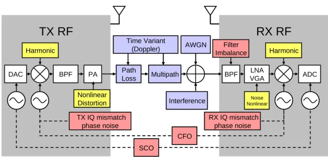
The MIMO-OFDM system supports BPSK、QPSK、16-QAM、64-QAM four kinds of modulation, FEC supports 1/2、2/3、3/4、5/6 four kinds of coding rate，and it can uses 2x2 or 4x4 antennas to transmit data. Before data transmitted, the data must go through Alamouti STBC（Space Time Block Code）encoding. After that, data go through OFDM modulation, and using IFFT to transfer frequency domain data to time domain signal. In each OFDM symbol, each symbol has 64 subcarriers , and 52 of them are data carrier, 4 of them are pilot carrier, others are null carrier. In receiver, first step, it uses FFT to transfer received signal to frequency domain data; second, Equalizer will compensate channel effect then combine two stream data into original by Alamouti Decoder. The MIMO basic architecture is as Fig.2-1 and the Alamouti STBC（Space Time Block Code）is as Fig.2-2. The basic MIMO-OFDM transmitter and receiver is as Fig.2-3 and Fig.2-4. And Fig2-5 shows the used system channel model. In this thesis, we focus on the path loss and interference, and the path loss model and interference model will be introduced in next section in detail

STBC Encoder/ Interleaver IFFT Information Bit IFFT H11 H22 H21 H12 FFT FFT Demodulator Equalizer Deinterleaver /Decoder Decoded Bits

1 , 1 h 2 , 1 h 1 , 2 h 2 , 2 h * 1D 2D X −X * 2D 1D X X time1 time2 1 1 1 * * 1 1D 11 2D 12 1 2 2D 11 1D 12 2 Y =X H +X H +W Y = −X H +X H +W1 time1 time2 2 2 2 * 1 1D 21 2D 22 1 2 2D 21 1D 22 Y =X H +X H +W Y = −X H +X H* +W2 2 1 , 1 h 2 , 1 h 1 , 2 h 2 , 2 h 1 , 1 h 2 , 1 h 1 , 2 h 2 , 2 h * 1D 2D X −X * 2D 1D X X time1 time2 * 1D 2D X −X * 2D 1D X X time1 time2 1 1 1 * * 1 1D 11 2D 12 1 2 2D 11 1D 12 2 Y =X H +X H +W Y = −X H +X H +W1 time1 time2 2 2 2 * 1 1D 21 2D 22 1 2 2D 21 1D 22 Y =X H +X H +W Y = −X H +X H +W 1 1 1 * * 1 1D 11 2D 12 1 2 2D 11 1D 12 2 Y =X H +X H +W Y = −X H +X H +W * 2 2 1 time1 time2 2 2 2 * 1 1D 21 2D 22 1 2 2D 21 1D 22 Y =X H +X H +W Y = −X H +X H* +W2 2

Figure2.2 Alamouti STBC（Space Time Block Code）

Figure2.3 MIMO Basic Transmitter

RX RF

TX RF

DAC BPF PA Path Loss Interference Multipath AWGN BPF LNA VGA Time Variant (Doppler) TX IQ mismatch phase noise ADC CFO Noise Nonlinear RX IQ mismatch phase noise SCO Filter Imbalance Nonlinear Distortion Harmonic Harmonic

RX RF

TX RF

DAC BPF PA Path Loss Interference Multipath AWGN BPF LNA VGA Time Variant (Doppler) TX IQ mismatch phase noise ADC CFO Noise Nonlinear RX IQ mismatch phase noise SCO Filter Imbalance Nonlinear Distortion Harmonic Harmonic

Chapter 3

Path Loss Model and Interference Model

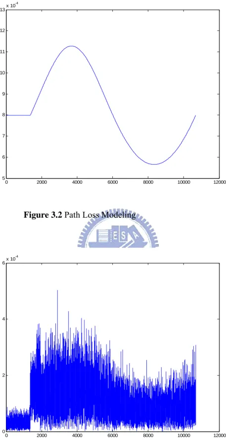
Because the signal power will decrease with the distance between TX and RX increasing, at the RX amplifier that needed is called Variable Gain Amplifier (VGA) to enhance the received signal power. If not, the wireless system will difficultly detect any signal. Assume that the transmitted signal is s(t) and the received signal is r(t), then path loss effect can be modeled as loss path t s t r( )= ( )* _

path_loss is a vibrated –n*db to +n*db and its value is from 0 dB to several hundred dB. If the path loss is very crucial, the receiver will be not able to detect any signal without VGA. However it is difficult to know that how exact the path loss is. So the goal of AGC is to estimate the suitable path loss effect and justify the VGA gain to let the system work under the situation of having steady signal.

0 2000 4000 6000 8000 10000 12000 0 0.05 0.1 0.15 0.2 0.25 0.3 0.35 0.4 0.45 0.5

0 2000 4000 6000 8000 10000 12000 5 6 7 8 9 10 11 12 13x 10 -4

Figure 3.2 Path Loss Modeling

0 2000 4000 6000 8000 10000 12000 0 2 4 6x 10 -4

Figure 3.3 The Received Signal With Path Loss

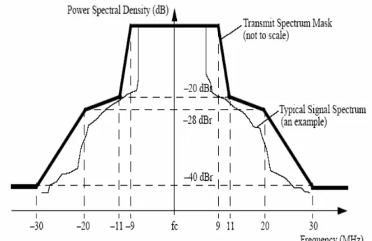
which is the interference of the first system. Generally there are two kinds of interference according there operation band. One is co-channel interference. For example, TDMA system is interfered by GSM/GPRS or NADC interference and their operation band are overlap. Another is adjacent channel interference (ACI). For example, UWB system is interfered with 802.11a interference and their operation bands are different. And our research focuses on adjacent channel interference (ACI).

Because of the spectrum mask is not perfect, there are some weak signal transmits from the infinite extended frequency. If ACI is much near our receiver than transmitter, the weak signal may be great for our receiver.

w

_I

f

_I

+w

_b

w

_b

f

_I

w

_I

f

_I

+w

_b

w

_b

f

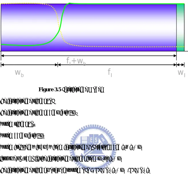
_I

Figure 3.5 Interference Model

The interference signal : SI

The interference signal bandwidth : wI

System signal : Ss

System bandwidth : wb

System frequency is away from interference operation band fI ~ fI + wb

First, we up-sample the interference signal from wI to fI + wb

The interference signal works on system SIS = LPF(SI, fI + wb)-LPF(SI, fI)

LPF(s,f) is signal s which is filtered by low pass filter which low frequency f can be pass

Then, we are down-sample SIS to wb from fI + wb

So, SIS is work on base-band of our system

System receive signal will be Sr = SS + SIS

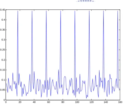
Our MIMO bandwidth is 20Mhz, we assume the interference bandwidth is 1Mhz, the high frequency composition of interference only appearance from one to zero and zero to one. So every 25 MIMO sampling point, interference will arise one time.

0 20 40 60 80 100 120 140 160 0 5 10 15 20 25

Figure 3.6 The Signal with Interference before ADC

0 20 40 60 80 100 120 140 160 0 0.05 0.1 0.15 0.2 0.25 0.3 0.35 0.4 0.45

Chapter 4

Timing Synchronization for MIMO system

4.1 AGC Control

For MIMO systems, the cross-correlator output is the most important information to estimate synchronized information, and the symbol power is also important information. Hence in MIMO system the correlation and symbol power is used to do this operation. The proposed AGC algorithm is base on the cross-correlation output and symbol power.

( )

_t

(

_s

( ) ( )

_{t ht e} ( ) _n

_{( )}

_t

)

_{path loss}

r _{= ⊗ •} j2π∆ft+θ _{+ * _}

Where s(t) is the received signal, h(t) is multipath impulse response, ∆f is CFO, θ is phase offset and n(t) is AWGN, path_loss is random number which is from -5db to -60db. This is general received signal present formula.

Before we detect the packet coming or not, we should adjust the noise power. My approach is adjusting the noise average power of 16 sampling points to take AD 1 to 2 bit. We hold the VGA value if the noise average power even take AD 1 to 2bit. If the noise average power is too small, we amplify the VGA n time until the noise take AD 1 to 2 bit. Sometimes the path loss is loss too many, we need more sampling points to adjust our noise average power.

After adjusting the noise power to a level we use the PAPR of cross-correlation value to decide the preamble VGA, if the PAPR of cross-correlation value is bigger than a threshold, we adjust the received signal power according the cross-correlation value. After adjusting the signal power, we start to do packet detection. Maybe the packet is still not coming. If the packet detection algorithm determines the packet still not coming, we should adjust the VGA to noise level, and continue to measure the PAPR of cross-correlation value to adjust VGA to preamble level circularly.

4.2 Detection of OFDM Packet

The OFDM Short preambles have been designed to help the detection of the start of the packet. These preambles are Pseudo Noise (PN) sequence in frequency domain, and they enable the receiver to utilize a very simple and efficient algorithm to detect the packet. The general approach was presented in Schimdl and Cox [6] using the special preamble composed of two identical symbols to synchronize the timing. And our MIMO system is according this algorithm to building our packet detection algorithm.

. The OFDM short training symbol r1(t)、r2(t) are used for the packet detecting. The cross-correlation function d1(t) and d2(t) is defined by

( )

1

(

) ( )

2 0 1 1

∑

− = ∗ + = Lb k k b k t r t d

( )

(

) ( )

Where r1(t+k) is the received signal of one antenna and r2(t+k) is received signal of another antenna, b(k) is the STF of transmitter, so d1(t) and d2(t) are the cross correlation with received signal and STF of transmitter.

2 1 0 2 2

∑

− = ∗ + = Lb r t k b k t d k

The packet detection formula is defined by

( )

t ∗d

( )

t ≥Γ

d1 2

Γ is the threshold which we pre-define, if the product of d1(t)*d2(t) is bigger than the

threshold , we determine the packet is coming, or the received signal is still noise.

According 4.1, we should adjust the received power to noise level. Γ

But there is a great problem for our packet detection algorithm, it is adjacent channel interference (ACI). If there is other communication system which works frequency band is different to our system near our receiver. It will hurt our packet detection, and always determine the packet coming but it’s not. So we need other algorithm to defend the ACI infecting.

if PAPR(i) > Δ S(i) = 0 else

S(i) = S(i)

PAPR(i) is the peak-average-power-ratio of the i-th sampling point, Δ is the PAPR threshold. If the power of sampling point is too big for average power, we will truncate the impulse to zero else hold the received power. If the ACI not appear too thickly, the information of the truncated short preamble is enough to do packet detection. Because loss one sampling point of STF, the property of cross-correlation does not change, so we use the

truncated algorithm is enough to do packet detection, but other parts of synchronization algorithm

will be not work, ex: IQ compensation、channel estimation.

4.3 Preamble

Compensation

Because of IQ compensation and channel estimation need precise preamble structures. The channel estimation uses the HT_LF, and the IQ compensation uses either HT_LTF or L-LTF. So after the packet detection we should precisely compensate the preamble which infected by ACI. If we don’t compensate the infected preamble, the IQ compensation and the channel estimation will be not work.

The IQ compensation uses L-LTF and HT_LTF, the format of L-LTF is presented by Figure1.

Because of L-LTF format is two same frames, and is the same in each antenna. Although each received L-LTF mixes two form of multi-path for each antenna. But because L-LTF is the same in each antenna, we can treat the mixed multi-path as another single multi-path. Because the L-LTF is circular, so the received L-LTF is also circular. Then if the

interference occurs, we can take the corresponding sampling points of another frame to compensate the sampling points which interference occurs.

The L-LTF compensation algorithm is presented by

Compensation of L-LTF algorithm is simple, because of L-LTF is circular. But compensation of HT-LTF isn’t same as the compensation of L-LTF algorithm, because of HT-LTF is not full circular. The sampling index of 1 to 144 is circular, index of 1 to 16 is GI, index of 17 to 80 and index 81 to 144 is the same frames. So compensating of index 1 to 144 of HT-LTF (HT-LTF1) we adopt the compensation of L-LTF algorithm, and we can precisely compensate the truncated HT-LTF1.

But the sampling index of 145 to 224 of HT-LTF (HT-LTF2) is only one frame, we can not compensate this part by another. We need other algorithm to compensate this part. The algorithm we use is “Time Domain Channel Response Algorithm” which uses the cross-correlation and orthogonal characterization to produce the time domain channel response. We use the time domain channel response to recover the truncated HT-LTF2. Using this algorithm we can availability produce the compensation frame which is like the HT-LTF which dose not infected by interference.

Now we introduce the time domain channel response algorithm, first we observe the

composition of HT-LTF2. The real part of 1st antenna HT-LTF2 is composed of real part of

1st transmitter HT-LTF2 after the real part channel H11, image part of 1st transmitter

HT-LTF2 after the image part channel H11, real part of 2nd transmitter HT-LTF2 after the

if PAPR(i) > Δ

if (sampling point is first frame)

S(i) = S(i+64)

else

S(i) = S(i-64)

else

real part channel H12, and image part of 2nd transmitter HT-LTF2 after the image part channel H12. And so dose the image part of H12, real part of H21, and image part of H21.

We observe the cross-correlation between real part of 1st antenna HT-LTF2 and real part

of 2nd antenna HT-LTF2, the cross-correlation between real part of 1st antenna HT-LTF2 and

image part of 2nd antenna HT-LTF2, the cross-correlation between image part of 1st antenna

HT-LTF2 and real part of 2nd antenna HT-LTF2, the cross-correlation between image part of

1st antenna HT-LTF2 and image part of 2nd antenna HT-LTF2. We can find the above

cross-correlation value almost approach zero, because of the orthogonal characterization. Now we know the composition of HT-LTF2 and the orthogonal characterization of HT-LTF2. We can use above information to reconstruct the HT-LTF2. First we do the

cross-correlation of real part of 1st antenna HT-LTF2 after truncated (figure 3.8) and real part

of 1st transmitter HT-LTF2, and cross-correlation of image part of 1st antenna HT-LTF2 after

truncated and image part of 1st transmitter HT-LTF2. This two cross-correlation is similar the

real part time domain channel response TH11. And so dose the image part time domain channel response TH11, the real part time domain channel response TH12, and the image part time domain channel response TH12.

0 10 20 30 40 50 60 70 80 -0.6 -0.4 -0.2 0 0.2 0.4 0.6 0.8

We can get the real part and image part of TH21, and real part and image part of TH22 by the same method.

After we get the time domain channel response, we can reconstruct the HT-LTF2 by convolution of time domain channel response and transmitter HT-LTF2.

We can get the real part of 1st HT-LTF2 by convolution of real part of 1st transmitter

HT-LTF2 and real part of TH11, convolution of image part of 1st transmitter HT-LTF2 and

image part of TH11, convolution of real part of 2nd transmitter HT-LTF2 and real part of

TH12, and convolution of image part of 2nd transmitter and image part of TH12. Adding all

the convolutions, we can reconstruct the real part of 1st HT-LTF2.

We can get the image part of 1st HT-LTF2 by convolution of real part of 1st transmitter

HT-LTF2 and image part of TH11, convolution of image part of 1st transmitter HT-LTF2 and

real part of TH11, convolution of real part of 2nd transmitter HT-LTF2 and image part of

TH12, and convolution image part of 2nd transmitter and real part of TH12. Adding all the

convolutions, we can reconstruct the image part of 1st HT_LTF2. We can also reconstruct the

real part and image part of 2nd HT-LTF2 by the same way.

Then we can use the reconstruct HT-LTF2 to compensate the HT-LTF2 which is infected by ACI. In complex channel condition, our ACI compensation algorithm work regular.

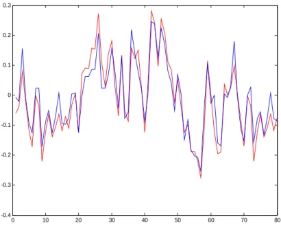
0 10 20 30 40 50 60 70 80 -0.4 -0.3 -0.2 -0.1 0 0.1 0.2 0.3

Figure 4.2 Red: Compensation Real Part of 1st HT-LTF2

Blue: After Truncated Real Part of 1st HT-LTF2. The Truncated Point is 21 41 61

4.4 Adaptive threshold

Now we return to the threshold decision problem. The false alarm probability is the area of noise curve above threshold; the packet loss probability is the area of OFDM curve below threshold. If the threshold sets too high, the false alarm probability decreases but the packet loss probability increases. On the other hand, if the threshold sets too low, the packet loss probability decrease but the false alarm probability increases. The trade off can be made by setting the threshold Γ at the intersection of OFDM and Noise curves.

In the adaptive threshold algorithm, we collect the cross correlation of noise and correlation of preamble after packet detection first. Then we normalize the correlation value. Last we use this information to define our new adaptive threshold. The adaptive threshold is useful for low SNR condition. If the original threshold we define is too small or too large, the adaptive can improve the original threshold.

Preamble

correlation pdf

Noise

correlation pdf

Correlation

Adaptive threshold

Figure 4.3 Adaptive Threshold Decision

4.5 AGC Tracking

The path loss is vibrated -3db to +3db. If we don’t track the path loss, the decoded data will be wrong. So we need algorithm to do the AGC tracking. We use the average pilot amplitude of this symbol to tune the VGA gain of next symbol. If the average pilot amplitude of this symbol is too large, we need to tune the VGA gain lower, vice versa.

0 2 4 6 8 10 12 14 16 18 20 0.2 0.3 0.4 0.5 0.6 0.7 0.8 0.9 1 1.1 1.2

0 2 4 6 8 10 12 14 16 18 20 0.8 0.85 0.9 0.95 1 1.05 1.1 1.15 1.2 1.25

Figure 4.5 Average Pilot Amplitude of 20 Symbols with AGC Tracking

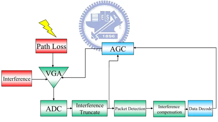
VGA

ADC

Interference_Truncate

Interference Packet Detection

AGC

Data Decode

Path Loss

Interference compensation

VGA

ADC

Interference_Truncate

Interference Packet Detection

AGC

Data Decode

Path Loss

Interference compensation

Chapter 5

Matlab Simulation

5.1 Simulation Platform

To evaluate the proposed algorithm, a typical MIMO-OFDM system based on IEEE

P802.11 Wireless LANs, TGn Sync Proposal Technical Specification, is used as a reference-design platform. The parameters used in the simulation platform are “The length of OFDM symbol is 64 and cyclic prefix is 16”.

The simulation result below is based on the 2x2 MIMO-OFDM systems in 20MHhz. PSDU is 1024, MCS is 13 (modulation is 64QAM, coding rate is 2/3 ), and using soft Viterbi decoder.

5.2 Simulation Result

We evaluate the performance of proposed packet detection, AGC control/tracking estimation, and ACI compensation algorithm in MIMO system. The simulation environment is under Rayleigh fading channel with RMS 100ns (TGnD) and 150ns (TGnE).The results are obtained by applying 1000 simulation runs with different SNR.

Figure 5.1 shows the packet error rate at 20MHz and RMS 100 ns (TGnD). Blue line is only channel effect. Red line is channel effect and path loss vibrates -3db to +3db. Magenta line is channel effect and ACI effect. Green line is channel effect, ACI effect and vibration effect. All the conditions run with different SNR. And the Figure 5.2 consider the IQ mismatch effect and frequency dependent imbalance (FDI) effect. We assume the IQ mismatch effect and the FDI effect are all worst case.

15 15.5 16 16.5 17 17.5 18 18.5 19 0 0.1 0.2 0.3 0.4 0.5 0.6 0.7 0.8 PER vs SNR SNR PE R none ACI+sin sin ACI

Figure 5.1 PER vs SNR, MCS13, TGnD, SIR 10db, path loss vibrates -3db to

+3db 19 20 21 22 23 24 25 0.05 0.1 0.15 0.2 0.25 0.3 0.35 0.4 PER vs SNR SNR PER none ACI sin ACI+sin

Figure 5.2 PER vs SNR, MCS 13, TGnD, SIR 10db, IQ mismatch and FDI effect

Figure 5.3 and 5.4 shows the packet error rate at 20MHz and RMS 150 ns (TGnE). Blue line is only channel effect. Red line is channel effect and path loss vibrates -3db to +3db. Magenta line is channel effect and ACI effect. Green line is channel effect, ACI effect and vibration effect. All the conditions run with different SNR. And the Figure 5.4 considers the IQ mismatch effect and frequency dependent imbalance (FDI) effect. We assume the IQ mismatch effect and the FDI effect are all worst case

15 16 17 18 19 20 21 22 23 0 0.1 0.2 0.3 0.4 0.5 0.6 0.7 0.8 0.9 1 PER vs SNR SNR PER none ACI sin ACI+sin

19 20 21 22 23 24 25 26 27 0 0.05 0.1 0.15 0.2 0.25 0.3 0.35 0.4 0.45 0.5 PER vs SNR SNR PER none ACI+sin ACI sin

Figure 5.4 PER vs SNR, MCS 13, TGnE, SIR 10db, IQ mismatch and FDI effect

worst case, path loss vibrates -3db to +3db

Figure5.5 shows our packet detection algorithm which combines the adaptive threshold. The packet detection error rate is at 20MHz and RMS 100ns. Path loss vibrates -3db to +3db, and MCS =13. The results are obtained by applying 2000 simulation runs with different SNR.

1 1.5 2 2.5 3 3.5 4 4.5 5 5.5 6 10-3 10-2 10-1 100 Packet_Detection_Loss v.s. SNR SNR P a c k et _D e tec ti on_ Lo s s

Chapter 6

System Architecture

The whole time synchronization architecture of proposed algorithms can be divided into four parts, the MIMO packet detection, symbol timing estimation, time domain channel response production, and ACI compensation.

Figure6.1 shows the architecture of MIMO packet detection. Figure6.2 shows the architecture of noise control. Figure6.3 shows the architecture of interference truncated. Figure6.4 shows the packet detection. Figure6.5 shows the architecture of boundary decision. Figure6.6 and Figure6.7 shows the architecture of preamble compensation.

Reg1 Reg2 … Reg16

Interference Truncate

reg1 reg2 … reg81 … reg129 … reg145 … reg160

Noise Control for AGC on Packet Detection Boundary Decision on Preamble Compensation Channel Estimation

Pilot1 Pilot2 Pilot3 Pilot4

1/4 IFFT Data Decode on BOUNDARY 542 110 L_LTF HT_LTF CFR ADC ADC AGC Interface Pilot

Access Tracking pilot / Initial pilot

Gain Buffer

Figure6.2 the Architecture of Noise Control

reg145 ……… reg157 reg158 reg159 reg160 b1 b13 b14 b15 b16 threshold ON

Figure6.4 the Architecture of Packet Detection

b7 b8 ……… b69 b70

64 sampling points sel

ect Sample Select reg87 reg88 reg89 reg154 reg155 … ……… ……… ………… … ……… ……… ………… Time Domain Channel Response 1st antenna HT_LTF2 real 1st antenna HT_LTF2 image 2rd antenna HT_LTF2 real 2rd antenna HT_LTF2 image

real/image select

Chapter 7

Conclusion and Future Work

7.1 Conclusion

In this thesis, we propose a packet synchronizer that can solve the path loss and adjacent channel interference which infect our MIMO system. We solve the path loss by average amplitude of pilot, and solve the ACI by “Time Domain Channel Response Algorithm”. We also construct the adaptive threshold algorithm to prevent the SNR varies too large. To hardware implementation, we design the system architecture. We will implement our hardware by this system architecture.

7.2 Future Work

There are some possible improvements in the future works. First, we although compensate ACI which infect the preamble, but the ACI infecting on data we still can’t solve it. So we should have other algorithm to compensate the data in future research.

Reference

[1] Shih-Lin Lo; “The Study of Front-End Signal Process for Wireless Baseband Applications” July 2004

[2] Jin-Hwa Guo; “Design and Analysis of Low Sampling Rate Packet Synchronizer in Dual OFDM/DSSS Wireless LAN” July 2005

[3] J.D. Laster and J.H. Reed; “Interference Rejection in Digital Wireless Communications ” 1997 IEEE

[4] Jiann-Ching Guey, Ali Khayrallah and Gregory E.Bottomley; “Adjacent Channel Interference Rejection for Land Mobile Radio Systems” 1998 IEEE

[5] Huseyin Arslan; “New Approaches to Adjacent Channel Interference Suppression in FDMA/TDMA Mobile Radio Systems” 2000 IEEE

[6] H.-F. Hsiao, M.-H. Hsieh, and C.-H. Wei, “Narrow-band interference rejection in OFDM-CDMA transmission system,” in Proc. IEEE International Symposium on Circuits and Systems, vol. 4, pp. 437–440, 1998.

[7] K. Fazel, “Narrow-band interference rejection in orthogonal multi-carrier spread spectrum communications,” in Proc. of International Conference on Universal Personal Communications, pp. 46 –50, 1994.

[8] E. Gunawan and Y. Zhu, “Performance of MC-CDMA system with power balance control over partial-band jammed multipath fading channels,” in Proc. of IEEE Vehicular Technology Conference, vol. 2, pp. 1485–1488, 2000.