Asynchronous parallel discrete event simulation

IEEE TRANSACTIONS ON SYSTEMS, MAN, AND CYBERNETICS-PART A: SYSTEMS AND HUMANS, VOL. 26, NO. 4, JULY 1996 397

Asynchronous Parallel Discrete Event Sirnullation

Yi-Bing Lin and

Paul

A.

Fishwick, Senior Member, ZEEE

Abstruct- Complex models may have model components dis- tributed over a network and generally require significant ex- ecution times. The field of parallel and distributed simulation has grown over the past fifteen years to accommodate the need of simulation the complex models using a distributed versus sequential method. In particular, asynchronous parallel discrete event simulation (PDES) has been widely studied, and yet we en- vision greater acceptance of this methodology as more readers are exposed to PDES introductions that carefully integrate real-world applications. With this in mind, we present two key methodologies (conservative and optimistic) which have been adopted as solutions to PDES systems. We discuss PDES terminology and methodology under the umbrella of the personal communications services application.

I. INTRODUCTION

UR purpose is to introduce the basic technical concepts

0

of distributed simulation of event-based models

(so

called discrete event models), and to tie these generic concepts to a specific application: personal communications services (PCS). Several introductory articles have been presented in the literature such as Fujimoto [l], Nicol et al. 121 and Richter et al. [3]. These papers have helped to disseminate the asynchronous parallel discrete event simulation (PDES) methodology for a wide readership. Our approach is similar but stresses a single real world application for discussing the methodology of PDES. By defining the methodology and all PDES terminology within the context of the PCS application, this paper serves both as a tutorial to PDES and as an introduction to PCS simulation modeling. PCS is a rich enough application to illustrate most basic PDES concepts.

The processing elements in PDES can either be of a parallel or distributed nature. An MIMD machine with multiple asyn- chronous elements performing message passing is an example of a parallel machine. Distributed elements normally refers to local or wide area networks composed of inter-connected set of heterogeneous workstations and computers. PDES is used for one of two reasons: 1) one wants to execute

a

model faster than is possible in a sequential machine, or 2) one must model in a distributed fashion because of a constraint that a process

Manuscript received January 15, 1995; revised July 25, 1995. This work was supported by the Rome Laboratory, Griffiss AFB, NY, under Contract F30602- 95-C-0267, and Grant F30602-95-1-003 1, the Department of the Interior under Grant 14-45-0009- 1544- 154, and the National Science Foundation Engineering Research Center (ERC) in Particle Science and Technology, University of Florida (with Industrial Partners of the ERC), under Grant EEC- Y:B. Lin is with the Dcpartment of Computer Science and Information Engineering, National Chiao Tung University, Hsinchu 300, Taiwan, R.O.C. (e-mail: liny@csie.nctu.edu.tw).

P. A. Fishwick is with the Department of Computer and Information Sciences, University of Florida, Gainesville, FL 3261 1 USA (e-mail: fish- wick@cis.ufl.edu).

94-02989.

Publisher Item Identifier S 1083-4427(96)0383S-6.

(i.e., computation) must be distributed rather ithan localized to a single processor. One author (Lin) has demonstrated various speedups possible on a distributed memory architecture for the PCS application [4], [5]. There is no question that PDES speeds up otherwise serial computations during a simulation. The second reason for PDES (distributed model constraint) is based on a situation where models for system components are stored in physically different locations. The other author (Fishwick) is building a prototype distributed simulation of a process plant where each plant component is ultimately co-located with the manufacturer of that component.

The paper proceeds as follows. First, in Section 11, we define our terms within the PDES area and demonstrate the generic approach to distributed simulation. In Section 111, we introduce the PCS application and demonstrate the need for synchronization of incoming messages to a given process. There are two key approaches to synchronization. Method

1, defined in Section IV, is termed the conservative method since it ensures that the causal relation among time consecutive events will be maintained at all times during the simulation. Method 2 is defined in Section V, and identifies the optimistic method. In this approach, the causal relation can be broken with subsequent fixing of state variables. We close in Section VI with directions for the future of PDES.

Throughout this paper, we use three font styles to represent different concepts. The typewriter type style represents attributes or methods (e.g., SendMessage ( ) ) of objects. The italic type style represents variables such as LP or p . The serif type style represents even1 types such as

Cal l A r r ival.

11. PARALLEL DISCRETE EVENT SIMULATION

A. Basic Terminology

We begin by defining terms which are commonly found in the simulation and PDES fields. These terms will be revisited in Section 3 when we assign the terms to the PCS application. The study of any physical system to be simulated begins with the creation of a model. Such a model can be in one of several types [6]: 1) conceptual, 2) declarative, 3) functional,

4) constraint, 5 ) spatial or 6) multimodel. One begins with a conceptual model which describes qualitative terms and class hierarchies for the system. In many ways, the conceptual model “organizes” the definition of attributes, methods and general characteristics of each system component without going so far as to ascribe dynamics to components. The next four model types reflect an orientation to system construction; a system may be constructed as a Petri net [7

1,

queuing model [8] or as a cellular automaton [9] for instance. The last model

39s IEEE TRANSACTIONS ON SYSTEMS, MAN. AND CYBERNETICS-PART A: SYSTEMS AND HUMANS, VOL. 26, NO. 4, JULY 1996

Output Channel Buffers

Fig. 1. Anatomy of a logical process (LP).

type (multimodel) permits the integration of basic model types to create a model composed of component models [ 101; [ 111 where each component model represents a level of abstraction for the system.

The PCS area, to be discussed in Section 3, uses a spatial model in that the system is viewed as a hexagonal discretiza- tion of a large two-dimensional space representing an area where cellular communications are to be implemented. Spatial models can be executed in several ways including time slicing, event scheduling and parallel and distributed. Our approach will be to use a parallel and distributed approach to model execution, while using the concept of event scheduling within each process. Speaking of process, we must define this term appropriately. Model components for a PCS implementation will be a collection of hexagonal cells. Other model types, such as a queuing model, are composed of other components (facilities). A logical process (LP) is defined as a set containing basic model components, so a PCS logical process will be a set of hexagons, or just one hexagon. A physical process or processor is

a

set of logical processes mapped in

a

way that conforms to the architecture of the parallel/distributed system.

An LP contains several objects:

Local Virtual Time (LVT): time associated with the LP. The LP does not know another LP’s time unless commu- nicated via

a

message.

Future Event List (FEL): event list used when there are internal events posted within the LP itself.

Event: an item within the FEL.

Message: an item sent from one LP to another. The FEL is composed of events, where an event combines the following objects: 1) time stamp, 2) token, 3) event type. The time stamp reflects when the event is to occur. An event’s occurrence correlates with the execution of an event routine for that LP. The token is associated with whatever is flowing through the network of LP’s. For the PCS application, portables (i.e., mobile phones) flow through the system. An event type specifies what will happen to the token (arrival, boundary crossing, departure, incoming call). An LP has input channels and output channels where each channel has a first- in/first-out (FIFO) buffer associated with it. A message is equivalent to an event that must be moved from one LP

to another. Messages which simply enter an FEL and are processed are generally called events. When an event must be issued to another LP, it becomes a message. The relationship among the above terms is shown in Fig. 1.

Messages arrive in one of several input channel buffers and are routed directly to the LP’s FEL. Note that simple LP’s may involve a calculation such as 1) taking the timestamp from an incoming message, 2) adding a value to this timestamp, and 3) sending the new message to the output buffers. Such an LP would not have any need of an FEL and would be a “pure” distributed simulation. This kind of technique, however, is wasteful of the computing elements since there will be a large price to pay in communications overhead among inter-LP communication. A simple addition is not sufficient to warrant a distributed approach. On the other hand, if the processing element can be made to do work then the communications overhead becomes less critical. The kind of work ideally suited in simulation is a sequential simulation within the LP, composed of the usual FEL and event routines. Thus, the distributed simulation is hybrid in

form with sequential simulation coinciding-and synchronized with-distributed simulation. The LVT of this more substantial LP is updated by removing the highest priority event (lowest timestamp) from the FEL and executing the associated event routine. Some (or all) of these event routines will contain scheduling commands to place events with new times back into the FEL. Some event routines will involve messages to be issued through the output buffer(s) to a target LP.

B. Object Oriented Implementation

A PDES consists of several PDES objects or LP’s. These LP’s execute asynchronously with coordination to complete a simulation run. To implement the objects in an LP (as described in Section 11-A), the attributes and methods of the LP are classified into four categories (see Table I):

A clock mechanism indicates the progress of the LP. An attribute LVT represents the timestamp of the event that just occurred in the LP. The LVTUpdate ( ) method updates LVT to advance the “clock” of the LP.

A FEL mechanism processes the events occurring in the LP. The FEL is basically a priority queue with one

LIN AND FISHWICK: ASYNCHRONOUS PARALLEL DISCRETE EVENT SIMULATION 399

Mechanism Clock FEL

TABLE I

ATTRIBUTES AND METHODS OF AN LP Attributes Methods LVT LVTUpdateO eventList Enqueue() Synchronization

I

1

D e q u e u e 0 Cancel() ReceiveHessageO SendMessageO

-

1

ExecuteMessageO

Application

1

to be elaborated

1

to be elaborated

attribute and three methods. An attribute eventLis t

maintains the events to occur in the future. The

Enqueue ( ) method inserts a time-tagged event into

eventList so that eventList maintains its ordered sequence. The Dequeue ( ) method deletes the event with the minimum timestamp in eventlist. The

Cancel ( ) method deletes the event with a specified timestamp in eventlist.

A synchronization mechanism interacts with other LP’s to coordinate the execution of PDES. The R e - ceiveMessage ( ) method receives messages from other LP’s (these messages will be inserted into the FEL for processing). The method ExecuteMessage ( ) executes events in the FEL. The SendMessageO

method sends output message (generated by the execution of events) to their destination LP’s.

It is probably more appropriate to consider Exe- cuteMessage ( ) as a method of the FEL. However, this method is affected by the PDES synchronization mechanisms to be described later. Thus the method is

classified as part of the synchronization mechanism. An application mechanism represents a sub-model for a

specific simulation application to be simulated by the LP (to be elaborated).

C. PDES Implementation Platforms

PDES systems have been implemented in different paral- lel architectures such as BBN Butterfly [ 121-1 141, Sequent [15]-[17], JPL Mark I11 [ l S ] , Simulated Stanford Dash Multi- processor [19], Transputers [20], [21], CM-l/CM-5 [22], KSR 1231, and iPSC/S60 1241. PDES has also been implemented in workstations connected by a local area network [4] which is widely available in both the industrial and the academic environments.

111. PERSONAL COMMUNICATION SERVICES We use personal communication sewice (PCS) network simulation to illustrate PDES functionality. A PCS network [25], [26] provides low-power and high-quality wireless access for PCS subscribers or portables. The service area of a PCS network is populated with a number of radio ports. Every radio port covers a sub-area or cell. The port is allocated a number of channels (time slots, frequencies, spreading codes or a combination of these). A portable occupies a channel for an incoming/outgoing call. If all channels are busy in the radio port, the call is blocked. In PCS network planning,

PCS network modeling (usually conducted by simulation experiments) is required to investigate the usage of radio resources. Since PCS network simulation is time-consuming, PDES effectively speeds up the process of PCS network simulation. Specifically,

The size of the PCS network under stud;! is usually large (e.g., thousands of cells). A typical sequential PCS sim- ulation run takes over 20 hours, while the corresponding PCS PDES takes less than 3 hours using 8 processors [4] Another popular parallel approach, the parallel indepen- dent replicated simulation [27]-[29] (running multiple simulation replications concurrently) does not work for PCS simulation. In most cases, the PCS designer is interested only in the behavior of the PCS network at the engineered workload (e.g., the workload at which the blocking probability is 1%). To calibrale the simulation at the engineered workload, the setup of input parameters for the next simulation run is dependenl on the previous run.

Now we describe the PCS model and its mapping to the corresponding PDES. For demonstration purposes, we describe a simplified PCS model without considering the details of the radio signal propagation issues (such as Rayleigh fading, co- channel interference, and so on). We assume that there are S cells in the PCS network, and on the average, there are n portables in a cell. Every port is allocated some number of channels. A portable resides at a cell for a period of time which is a random variable with some distribution (e.g., exponential 1301-[32]). Then the portable moves to a neighbor cell based on some routing function (e.g., equal routing probabilitiec for all neighbors). The call arrivals to a portable is a random process (e.g., Poisson), and is independent of the portable’s movement. A call is connected if a channel is available. Otherwise, the call is blocked. When a portable moves from one cell to another while a call is in progress, the call requires

a new channel (in the new cell) to continue. This procedure of changing channels is called handoff or automatic link transfer (ALT). Several handoff schemes have been proposed in the literature 1331-[35]. In this paper, we constder the simplest scheme called nonprioritized scheme. In this scheme, if no channel is available in the new cell, then the call will be dropped or forced terminated immediately.

The PCS example is probably more realistic to the reader if we add some geometry to these moving vehicles (portables). Unfortunately, whether a vehicle moves from one cell to an- other cannot be simply determined by the physical movement of the vehicle. We also need to consider the radio propagation. It is possible that the connection to a vehicle (changes from one port to another even if the vehicle is stationary-the change of radio signal strength may result in re-connecting the vehicle to a different port. According to the PCS network measurement methods, we determine that the movement (in the cense of port connection) of a vehicle is best characterized by the residence time’ distribution and the destination cell routing probability. The reader may image that this movement model is equivalent to a simple path approach where a vehicle maves straight with

400 IEEE TRANSACTIONS ON SYSTEMS, MAN, AND CYBERNETICS-PART A: SYSTEMS AND HUMANS, VOL. 26, NO. 4, JULY 1996

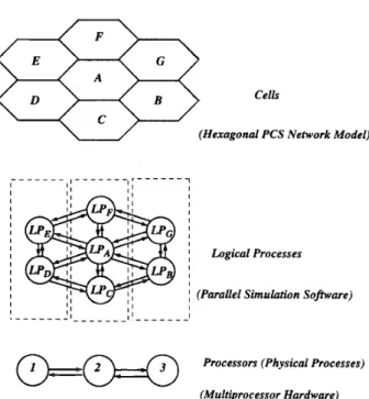
Cells

U

(Hexagonal PCS Network Model)

I I I I I I I I I I I I I I I I I I I

,

I

I

Logical Processes

I

I

(Parallel Simulation Software)

I I I

I I

Processors (Physical Processes)

o=o

_{(Multiprocessor Hardware)}

Fig. 2. Cells, logical processes, and processors. A PCS cell is represented

by a logical process (LP) in PDES. More than one LP may be mapped to a processor for execution.

an angle. The angle determines the destination cell and the residence time is the product of a constant speed and the diameter of the cell’.

To map the PCS model into PDES, the cells in the PCS network are represented by cell objects derived from the PDES objects (i.e., LP’s). These LP’s are then mapped to processors for execution (see Fig. 2). A cell LP has the following attributes and methods (i.e., the application mechanism of a general LP): A constant attribute channelNo represents the total number of channels in a radio port. An attribute

idleChannelNo represents the number of idle radio chan- nels. A portableList collects the information of all porta- bles reside in the cell. There are five methods in the cell object:

CallArrival(), CallCompletion(), Portable- MoveIn ( ) , PortableMoveOut ( ) , and Handof f ( ) . These methods will be elaborated later.

The portables in the PCS network are represented by the portable objects. A portable object consists of four attributes: * The busy attribute indicates the status of the portable. If

busy=YES then the portable is in a conversation. The callArrivalTime attribute represents the next call arrival time.

* The callCompletionTime attribute represents the completion time of the current phone call when

busy=YES. If busy=NO, the callCompletionTime

attribute is meaningless.

* The portableMoveOutTime attribute represents the time when the portable moves out of the current cell. There are two categories of events in a PDES. An internal event is scheduled and executed at the same LP (the event

’But note that our movement model is practical-it is used to approximate

real radio systems, unlike the simple path approach.

represents the interaction between a cell and a portable within the cell in our PCS example), and an external event is scheduled by one LP and is executed by another LP. Thus, after its creation, an internal event is inserted in the FEL by using the Enqueue ( ) method, and an external event is considered as a message, and is sent to the destination LP by using the Senmessage ( ) method. In the PCS PDES, there are three internal event types and one external event type. The internal event types are described below.

CallArrival: Either the port (the cell) or the portable initiates a call setup. A radio link is required to connect the port and the portable. If no radio link is available or the portable is already busy with another conversation, the call is dropped.

Callcompletion‘: A phone call completes, and the ra- dio link between the port and the portable is disconnected.

PortableMoveOut: The portable moves out of a cell. If the portable is in a conversation, the radio link between the portable and the port is disconnected.

We treat the CallArrival event type as an internally gen- erated event based on a probability distribution. This is just an abstraction of the actual situation where arrivals are sent from outside the LP to one of the LP’s input channels. Therefore, a more detailed simulation would involve “electromagnetic messages” reflecting the true nature of incoming calls. The use of a probability function is an abstraction for this underlying process.

The external event type is described below.

PortableMoveIn: A portable moves in a new cell. If the portable is in a conversation, then a new radio link between the cell (port) and the portable is required. If no radio channel is available, the call is forced terminated. In PDES, the execution of a PortableMoveOut event at a logical process

LPA

always results in the scheduling of a

PortableMoveIn event for the destination logical process L P B . This event type is external (to L P B ) , and the scheduling of the event requires communication between

LPA

and L P B .

An event/message m is of the format m = (timestamp,

p ,

eventType)

where eventType represents the type of the event, timestamp represents the (simulated) time when the event occurs, and

p

is the pointer which points to the corresponding portable

p . The execution of the event message m at a cell object LP is described as follows. The LP. ExecuteMessage ( ) method invokes different methods according to the event type of m (the Pascal-like “case” statement is used in the definition shown at the bottom of the next page). The methods invoked in

ExecuteMessage ( ) are described below. When the event type of m is CallArrival, the following action is taken.

CallArrival ( p ) { if p.busy=YES then

/* A call is already in progress when the new */ /* call arrives at LVT. In other words, a busy line */ /* occurs and the new call arrival is ignored. */ update the busy line statistic;

LIN AND FISHWICK ASYNCHRONOUS PARALLEL DISCRETE EVENT SIMULATION 40 1

if

idleChannelNo = 0 then

/* The call arrival is blocked. */

update the blocking statistic;

else /* I.e., idleChannelNo> 0. */

idleChannelNo t idleChannelNo -1; p.busy + YES;

generate the call holding time

t ,

and

p.callComp1etionTime + LVT

+

t ;

end if end if

generate the next inter-call arrival time

t’

and compute the next call arrival time as

invoke ScheduleNewEvent ( p ) ;

I* Schedule a new event (to be described). */

p.callArrivalTime +- LVT

+

t’.

1

Note that the busy line and call blocking statistics are output measures of the PCS simulation (not shown in our PDES

exarnp~e)~.

When the event type of m is CallCompletion, the following action is taken.

Callcompletion ( p )

{

/* Release occupied channel at call completion. */

idleChannelNo+-idleChannelNo+l;

p. bu s y=NO ;

invoke ScheduleNewEvent ( p ) ;

/* Schedule a new event (to be described). */

1

When the event type of M is PortableMoveIn, the follow- ing action is taken.

PortableMoveIn ( p ) {

if

p.busy=YES then /*

A

handoff occurs. */ invoke Handof f ( p ) ; /* To be described. */

end if

generate the portable residence time

t

and compute the next move time p.portableMove0utTimet LVT+t;

invoke ScheduleNewEvent ( p )

I* Schedule a new event (to be described). */

}

The method Handof f ( ) is described below.

Handoff ( p )

{

if idleChannelNo=O then

/* No channel is available to connect the */ /* handoff call i.e., the handoff fails. */

Call blocking is a major performance measure of a PCS network. A PCS network is usually engineered at 1% or 2% blocking probabilities.

update the forced termination statistic (not shown in our

PDES

example);

p.busy=NO;

id1 eChanne l N o t id1 eChanne 1No- 1; else /* The handoff succeeds. */

end if

}

If the event type of

m

is PortableMoveOut, the following action is taken.

PortableMoveOut ( p )

{

if p.busy=YES then

idleChannelNo+idleChannelNo+l; /* When a communicating portable moves */

/* to a new cell, it releases the occupied */ /* channel of the old cell. */

end if

determine the destination cell ( L P ’ ) to which the portable moves;

generate an output message

m’ = (LVT,p,PortableMoveIn) ; invoke SendMessage (m’, L P ‘ ) ;

/*

A

PortableMoveIn event is scheduled for LP’. */

}

Note that the timestamp of

m’

is the same as; that of m.

In our implementation, the execution of the event message

m

results in the scheduling of exactly one future event

m’. When m is executed, one or more attributes of the corresponding portable are updated. Then the next event for the portable is determined based on the updated values of the attributes.

If

the event type of m is PortableMoveOut,

then a PortableMoveIn event message with the same timestamp is scheduled for the destination LP as described in the definition of PortableMoveOut ( : I . For the other three event types, the message m’ =

( t s ,

0,

eventType’) is determined by invoking ScheduleNewEvent ( :

ScheduleNewEvent ( p )

{

if p.busy=NO then

I* The portable is idle at LVT. The next * I /* event occurring to p is either a call arrival */ /* or a cell crossing movement. */

ts t min(p. CallArrivalTime, p.portableMoveOutTime); if t s = p. callArrivalTime then

m’. eventType’ tCallArriva1; else m’. eventType’ t Portabl eMoveOut ; end if ~ ExecuteMessage ( m )

{

LVTUpdate(m. timestamp) /* I.e., L V T t m.timeStamp. */ case (m. eventType) of

CallArrival: invoke CallArrival (m.p) ;

Callcompletion: invoke Callcompletion (m.p) ; Port ableMove In: invoke Port ableMove In (m.p ) ; Port ab1 eMoveOu t : invoke Port ableMoveOu t ( m.p ; end case

402 IEEE TRANSACTIONS ON SYSTEMS, MAN, AND CYBERNETICS-PART A: SYSTEMS AND HUMANS, VOL. 26, NO. 4, JULY 1996

\

/

Legend:

portable (cross-boundary) movement call m ' v a l call completion Fig. 3. A simple PCS example.

else /* I.e., p.busy=YES. The portable is busy at */ callCompletionTime= ?, portableMoveOutTime=16

/* LVT. The next event occurring to p is either a */

/* call arrival, a call completion or a cell crossing */ and an event

/* movement. */

t s + min(p. callArrivalTime,

p.callCompletionTime, p.portableMove0utTime); if t s = p . callArrivalTime then

m' . eventType' +C a1 1Ar r iva 1;

else if t s = p . callCompletionTime then m'. eventType' t e a l lcompl e t

i

on;

else m'. eventType' i- Por t ableMoveOut ;

end if end if

1

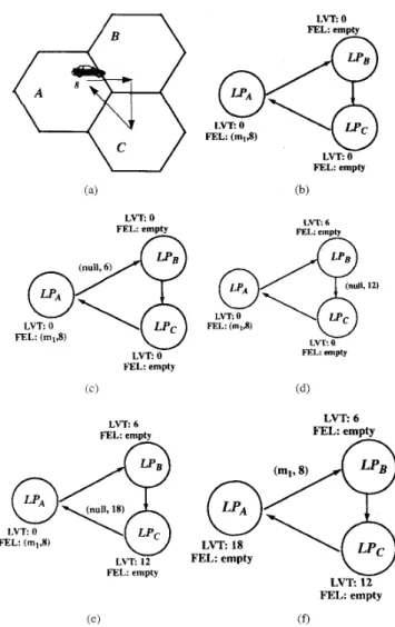
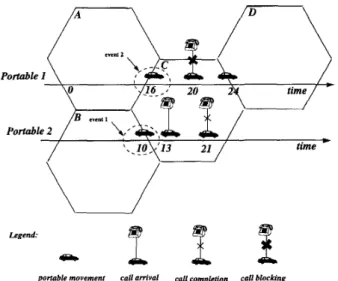
Consider the example illustrated in Fig. 3. In this figure, a portable is represented by a car (although in many PCS

systems, portables are carried by pedestrians). A call arrival is represented by a phone connected to the car. A call completion is represented by a cross (disconnection) on the phone line.

At time 0, portable p l is at cell A . At time 10, a phone call for p l occurs. The call completes at time 13, and the portable moves to cell B at time 16. At time 20, another phone call for p l arrives. At time 24, p l moves to cell C (and a handoff occurs).

In PDES, cells

A . l?,

and C are simulated by logical process

LPA.

LPB,

and

LPc

respectively. At the beginning of the

simulation, the attributes of p l are busy = NO,

callArrivalTime = 10,

ml =

(1O,pl,

CallArrival)

is scheduled and inserted in the FEL of LPA. When the LVT

of

LP;1

advances to 10, ml is executed by invoking

LPA.

CallArrival ( p l ) . Suppose that an idle channel exists. The call is connected and the call holding time for the conversation is generated (which is 3, or the call completion time is 10

+

3 = 13). The next call arrival time is also generated (which is 20 in Fig. 3). Thus the attributes of p l are modified as

busy = YES,

callArrivalTime = 20, callCompletionTime = 13, portableMoveOutTime =16

and a new event

m2 = (13,&, CallCompletion)

is scheduled and inserted in L P A ' s FEL. When the LVT of L P A advances to 13, m2 is executed. The method L P A . Callcompletion ( P I )

is

invoked and the attributes of p 1 are modified as

busy = NO,

callArrivalTime =

20,

callCompletionTime=?, portableMoveOutTime=16

and a new event

403 LIN AND FISIIWICK: ASYNCHRONOUS PARALLEL DISCRETE EVENT SIMULATION

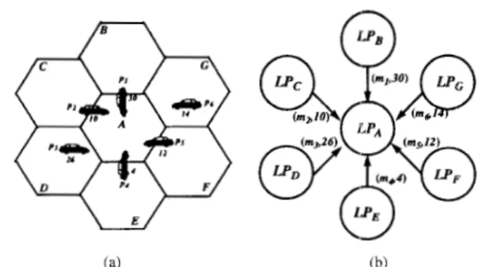
Fig. 4. PDES synchronization problem

is scheduled. At LVT 16, rn3 is executed. The method

LPA.

PortableMoveOut ( p l ) is invoked to determine the desti- nation cell (which is

B

in Fig. 3), and a message

rnl = (16, i PortableMoveIn)

is sent from LPA to LPB by invoking

LP,4.SendMessage(mJ4,

L P B ) .

Note that the portable p l migrates to

LPB

when rn4 is sent. (In GITBellcore’s

PCS implementation 141, a message is part of a portable object, and sending a message automatically migrates the corresponding portable object.) When

LPB’s

LVT advances to 16, it executes m4. The next portable move time is generated (which is 24). The attributes of pl are modified as

busy = NO,

callArrivalTime =

20,

callCompletionTime=?, portableMoveOutTime=

24

and a new event rn5 = (20,pl, CallArrival) is scheduled.

A PDES is correct if the following rule is satisfied. Locul Causality Constraint Every LP processes events in nondecreasing timestamp order.

The major problem of PDES is that the logical processes are executed at different speeds. Consider the scenario in Fig. 4 that portable pl moves from cell

A

to cell B at time 20 with an ongoing phone call (i.e., a handoff call), and portable

p 2 moves from cell

C

to cell

B

at time 13 with an ongoing phone call (see Fig. 4(a)).

Consider the PDES scenario in Fig. 4(b).

LPA

sends a PortableMoveIn event (message) ml (for p 1 ) with time- stamp 20 to LPB. Later

LPc

sends m2 (for p ~ ) with time-

stamp 13 to LPB. If

LPB

executes ml before m2 arrives,

then the modifications to

LPB.

idleChannelNo is out of the timestamp order, and the local causality rule is violated. Thus the simulation result is not correct.

To solve this problem, the executions of the logical pro- cesses must be synchronized. The remainder of this paper describes two popular asynchronous synchronization mecha- nisms, the conservative and the optimistic methods.

(a) (b)

Fig. 5.

time when the portable crosses the cell boundary.

The input waiting rule. In (a), the number below a car represents the

two rules: the input waiting rule and the output waiting rule. It also assumes that

the messages are received in the order they are sent (the FIFO communication properly), and

the communication channels among LP’s are fixed and never change during the simulation. In Fig. 4(b),

LPA

(LPc)

has one output channel directed to

LPB,

and

LPB

has two input channels (one from

LPA

and one from

LPC).

A. Basic Synchronization Mechanism

In a conservative simulation, every logical process

LP

Step 1.

LP

waits to select an input message m from its input channels (extra data structures are required to implement input channels in a logical process) by invoking

LP.ReceiveMessage ( )

.

This method is implemented based on the input waiting rule to be described. The method inserts

m

into

LP’s

FEL.

Step 2. Let

t s

be the timestamp of rn.

LP.ExecuteMessage ( ) is invoked to process all events in the FEL with timestamps no larger than t s in nondecreasing timestamp order. The execution may invoke

LP.SendMessage ( ) to send output messages. This method is implemented based on the outpiit waiting rule to be described. If the termination condition is satisfied (e.g.,

LP.LVT>5000), then exit the loop. Otherwise go to Step 1.

The waiting rules are described as follows.

The Znput Waiting Rule: An LP does not process any input message until it has received at least one message from each of its input channels. The input message with the smallest timestamp is selected for processing. Fig. 5 shows how the input message is selected for the PCS simulation.

Fig. 5(a) illustrates a PCS system where 6 portables

p 1 , p a , p 3 , p4, p 5 , and p6 move from cells B, (2, D, E, F, and G to cell A at times 30, 10, 26, 4, 12, and 14, respectively. In the PDES model (see Fig. 5(b)), the PortableMoveIn events

of p l

, . . . .

p6 are represented by the messages rnl,

. . .

. m6 sent to

LPA.

By the input waiting rule, r n 4 is Ihe next message

to be executed in

LPA.

Assume that all messages sent from one LP to another are in nondecreasing timestamp order (this property will be repeats the following two steps.

1V. CONSERVATIVE METHOD

The conservative simulation [36] is conservative in the sense that it does not execute an event before it ensures that the local

-404 IEEE TRANSACTIONS ON SYSTEMS, MAN, AND CYBERNETICS-PART A. SYSTEMS AND HUMANS, VOL. 26, NO. 4. JULY 1996

30 20 10 36 29 24

b

pomble am’vals portable deparmres

LVT: 0

FEL: emDh

LVT: 10

FEL: (m’,,29)

Step 1. Before ml is processed Step 2. After rnl is processed

LVT 20

F R L lm’,,24l (m’,,ZP) LVT 20

F R L lm’,,24l (m’,,ZP)

W

Step 3. After rn2 is processed Step 4. After rn3 is processed ib)

Fig. 6. The output waiting rule.

guaranteed by the output waiting rule to be described next), then the input waiting rule ensures that the timestamp of the selected message is no larger than any input messages to be processed in the future.

The Output Waiting Rule: An LP does not send an output message to another LP until it ensures that no output messages with smaller timestamps will be scheduled (at LP) in the future. Assume that all input messages are handled in nondecreasing timestamp order (the property is guaranteed by the input waiting rule). The output waiting rule is satisfied if an LP

only sends output messages with timestamps no larger than its current LVT value.

Consider the following PCS example. Portables p l

,

p 2 and

p~ move into cell A at times 10, 20, and 30, and move out

of the cell at times 29, 24, and 36, respectively (see Fig. 6(a)). This situation occurs since a portable, once inside cell A, may take a dramatically different from other portables. Some portables may stay in the same physical location for a period while other portables continue moving toward an adjacent cell to A.

In PDES, ml. m2, and m3 are input messages representing

the arrivals of p 1 , p z and p 3 , respectively (see Step 1 in Fig. 6(b)). When ml is processed, a move event

mi

for p l is scheduled with timestamp 29 (see Step 2 in Fig. 6(b)). In the conservative simulation,

mi

cannot be sent to the destination LP immediately, or the output waiting rule may be violated. In our PCS PDES implementation, the portable move is simulated by two types o f events: a Portable- MoveOut event and a PortableMoveIn event. In Fig. 6(b), rn; and

mt

represent the PortableMoveOut event and

PortableMoveIn event of portable p , , respectively. When the event m; is scheduled, it is inserted in LP;l’s FEL. When the LVT of LPA advances to the portable “move time” (i.e., the timestamp of ml), rn; is processed, which results in sending

LVT: 0 FEL: empty FEL: (m1,8) LVT 0 LW. 0 FEL: empty E L : (mlb) LVT 0 E L : empty i c ) LVT 6 FEL: empty E L : (ml,8) LVT: 12 FEL: empty LW. 6 FEL: empty LVT: 0 FEL: (m,,S) LW. 0 FEL. empty id) LVT 6 FEL: empty LVT: 18 FEL: empty LVT 12 FEL: empty (e) (0

Fig. 7. Deadlock and deadlock resolution.

the PortableMoveIn event

rnt

(with the timestamp of

m;)

to the destination. In Fig. 6(b), rn; and

my

are sent after Step (3) and before Step (4); i.e., when

LP;l

is sure that next input message to be handled has timestamp larger than

mi

and

m;.

Note that

m i

is sent before my is.

Since the output waiting rule is guaranteed by using the two “move” event types, the conservative SendMessage ( ) method simply sends the output message to the destina- tion. Note that for other applications, a different conservative

SendMessage ( ) method may be required to implement the output waiting rule.

The correctness of the conservative simulation can be proved by induction on the interaction of the two waiting rules.

B. Deadlock and Deadlock Avoidance

The input waiting rule may result in deadlock (LP’s are waiting for input messages from each other and cannot progress) even if the simulated system is deadlock free.

Consider a three-cell PCS network (see Fig. 7(a)). There is one portable in the network, and the portable moves in the path A i B + C + A . At time 0,

LIN AND FISHWICK ASYNCHRONOUS PARALLEL DISCRETE EVENT SIMULATION 405

the portable is in cell A. The portable moves form cell

A to cell B at time 8. In the conservative simulation, a PortableMoveOut event rnl is scheduled in LPA initially (see Fig. 7(b)). By the input waiting rule, L P A waits for an input message from L P c before it can process ml. Simi-

larly, L P c does not send out any output message before it receives an input message from L P B , and LPB does not send out any output message before it receives an input message from L P A (i.e., before rnl is processed). Thus the

PDES is in the deadlock situation. Two deadlock resolutions have been proposed: deadlock avoidance [36] and deadlock detectiodrecovery [37], [38]. It has been shown [39] that the cost of deadlock detection/recovery is much higher than deadlock avoidance. This article will focus on the deadlock avoidance mechanism.

In a PCS network, a portable is expected to reside in a cell for a period of time before it moves. Assume that every portable resides in a cell for at least six time units before it moves to a new cell. The information that “a portable resides in a cell for at least 6 time units” is used in the deadlock avoidance mechanism to predict when an LP will receive an input message, and “6 time units” is referred as the lookahead value. The lookahead information is carried by the control messages called null messages. A null message does not represent any event in the simulated system. Instead, it is used to break deadlock as well as to improve the progress of

a conservative simulation.

In Fig. 7(b), at the beginning of PDES, the LVT’s of the three LP’s are 0, and a PortableMoveOut event ml with timestamp 8 is in LPA’s FEL. At time 0, L P A sends a null message with timestamp 0

+

6 = 6 (the LVT value plus the lookahead value) to L P B (see Fig. 7(c)). The null message implies that no portable will move in cell B earlier than time

6. Thus, the LVT of L P B advances to 6 when the null message arrives (Fig. 7(d)). Since no portable arrives at cell B before time 6, it implies that no portable will move out of cell B before time 12 and L P B sends a null message with timestamp 12 to L P c . After the sending of several null messages, L P A will eventually receive a null message with timestamp larger than 8 (see Fig. 7 ( e ) ) , and by the input and output waiting rules, rnl is sent from L P A to L P B and the deadlock is avoided (see Fig. 7(f)).

C. Exploiting Lookahead

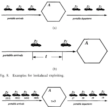
It is important to exploit the lookahead to improve the progress of a conservative simulation. Experimental studies have indicated that the larger the lookahead values, the better the performance of the conservative simulation [39]. Based on the techniques proposed in [40]-[42], we give three PCS examples for lookahead exploration. The first two examples assume single cell entrance and exit. The single entrancelexit PCS model has been used in modeling highway cellular phone systems [43]. The results can be easily generalized for multiple entrances and exits. The techniques introduced can be combined to exploit greater lookahead.

1. Lookahead Method 1 (FIFO): In a large scale PCS network, a cell may only cover a street, and the portables

leave the cell in the order they move in (the FIFO property; see Fig. 8(a)).

Consider the corresponding FIFO LP for cell A in PDES. The lookahead for the LP can be derived by a presampling technique proposed by Nicol [41]. The idea is to presample the residence tirnes of the arrival portables.

If the FEL is not empty, then the next departure time can be easily computed. In the PCS PDES, the move- out timestamp of a portable is computed and stored in

portableMoveOutTime of the portable object at the time when the PortableMoveIn event is processed. The FIFO property guarantees that the next departure time is the minimum of the portableMoveOutTime

values of portable objects in the FEL. ‘Thus, the precom- puted next departure times can be used as the lookahead. If the FEL of the LP is empty at tiniestamp LP.LvT, then the lookahead can be generated by the same pre- sampling technique. Since the portalole will arrive at the cell later than LP.LvT, it will leave the cell later than

LP.LVT

+

t

(where

t

is the prcsampled portable residence time). The FIFO property guarantees that after time LP.LvT, no portables will depart earlier than L P . L v T + ~ , and the LP may send null messages with this timestamp to the downstream LP’s.

2. Lookahead Method 2 (Minimum Inter-Boundary Cross-

ing Time): Consider the example in Fig. 8(b) where the FIFO portable movement property in the previous example does not hold. In practice, the inter arrival times to the cell (for the portables from the same entrance) cannot be arbitrary small. Instead, a minimum cell crossing time I- is assumed. Let p i (i = 1 , 2 , 3 ,

. .

.)

be the ith portable arrival after time LP.LvT. The portable residence time for p i is

ti.

Then the departure time of p i is later than LP.LVT

+

(i - 1)‘

+

t i , and the next departure time at the cell after LP.LVT is later than LP.LVT

+

A where

l<i<CC

A = rnin [(i -

I)‘+

t i ] . (1)

Since T

>

0, there exists j such that

1 S i S j

j~

2

min [(i - 1)‘

+

t;]

=

A.

In other words, to compute A it suffices to consider the first j presampled residence timestamps in (1). Fig.

9 displays a situation where we employ formula (1). Four portables arrive using times llD, 14, 19 and 22. Let I- = 3 so that we know that n’o two consecutive portable arrivals will be less than 3 . The residence times for the portables are placed in parentheses in Fig.

9. The variable j is increased by 1 until the above inequality is satisfied. Suppose that LPA needs to send a null message to its downstream before it receives the

PortableMoveIn event for p l . The residence times of the subsequent arriving portables are pre-samples as

tl

= 9 , t 2 = 4 , t 3 = l ; t 4 = 5 . .

.

Our algorithm proceeds as follows:

(a) For j = I, 1 x 3

2

min[0

+

91 = 9 ? NO. (b) For j = 2, 2 x 3

2

min[0

+

9 , 3

+

41 = 7 ? No.

406 lhEE TRANSACTIONS ON SYSTEMS, MAN, AND CYBERNETICS-PART A SYSTEMS AND HUMANS, VOL 26, NO 4, JULY 1996

t

portable am’vals

(b) Fig. 8. Examples for lookahead exploiting.

pomblc om’volr \ / p o d l e d e p a m r r e s

Fig. 9. Portables entering and leaving cell A

(c) For j = 3, 3 x 3

2

min[0

+

9 , 3

+

4.6

+

11

= 7

From this procedure, we derive

A

= 7 by using the first three pre-sampled residence times.

3 . Lookahead Method 3 (Minimum Residence Time): If the FIFO portable movement property does not preserve, and ‘T does not exist (or is too small to be useful), then the technique proposed in the previous example may not work. In a PCS simulation, the total number N =

S

x 7 1

of portables is an input parameter. To compute the next lookahead value for an LP, it suffices to sample the next

N portable residence times, and (1) is re-written as [42]

? Yes.

A

= min

t ,

l < i < N

The last two examples may require a large number of opera- tions to generate a lookahead value. In [40], O(1) algorithms have been proposed to generate the lookahead values.

When the ExecuteMessage ( ) method processes a null message in an LP, it invokes a method ComputeLooka- head ( ) to compute the timestamp of the output (null) mes- sages. The ComputeLookahead ( ) method may implement the lookahead exploiting techniques described above. Then the new null message is sent to some or all output channels by

invoking the SendMessage ( ) method.

V. OPTIMISTIC METHOD

The optimistic simulation [44] is optimistic in the sense that it handles the arrival events aggressively. When a message m arrives at an LP, LP.ReceiveMessage ( ) simply inserts

m

in the input queue (the optimistic simulation terminology for the FEL). The logical process assumes that the events already in its input queue are the “true” next events. The Exe- cuteMessage ( ) method proceeds to execute these events in

timestamp order, and SendMessage ( ) is invoked whenever an output message is scheduled. When a message arrives at the LP, the timestamp of the message may be less than some of the events already executed. (This arrived message is referred to as a straggler.) The optimism was unjustified, and therefore a method Rollback ( )

is

invoked by ExecuteMessage ( )

to cancel the erroneous computation. To support rollback, data structures such as the state queue and the output queue are required (to be elaborated).

Several strategies for cancelling incorrect computation were surveyed by Fujimoto [45]. Two popular cancellation strategies called aggressive cancellation [44] and lazy cancellation [46] are described in this section.

A. Cancellation Strategies

Consider the example in Fig. 10. For simplicity, assume that cell C has one radio channel (i.e., LPc.channelNo= 1 in

PDES). In this example, portable p 2 moves from cell B to cell C at time 10 (event l), and make a phone call at time 13. The call is completed at time 21. Portable 1 moves from cell A to cell C at time 16 (event 2), and attempts to make a phone call at time 20. Since the only radio channel is used by portable 2, the call attempt from portable 1 is blocked. Portable 1 moves from cell C to cell D at time 24. Figs. 1 1, 12, and 13 illustrate the data structures of

LPc

(the logical process corresponding to cell C) assuming that message ‘m1 (the message that represents event 2) arrives at

LPc

earlier than message mg (the message that represents event 1) does. In LPc, a state queue and an output queue are maintained to supported rollback. In our example, the state variable (attribute) for LPc is the number of idle channels LPc.idleChannelNo. The state variable is checkpointed and saved in the state queue from time to time. The snapshots in the state queue are used to recover the state of

LPc

when rollbacks occur. The output queue records the anti-messages of the output messages that have been sent from

LPc.

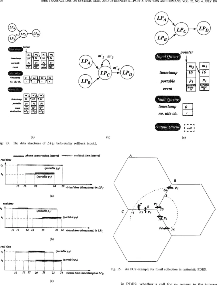
The anti-messages are used to annihilated false messages sent in the incorrect computation.

In Fig. l l ( a ) ,

LPc

receives m1 that is inserted in

LI‘c’s

input queue. Initially, the output queue of LPc is empty, and the value of LPc.idleChannelNo at timestamp 0 is saved. After ml is executed, the system state at timestamp

16 is checkpointed, and a call arrival event (message m 2 ) is scheduled for LPc itself (see Fig. 11 (b)). Note that after its execution, ml is kept in the input queue (this message may be re-executed if a rollback occurs). A pointer in the input queue indicates the next event to be executed. The anti-message m; of m2 is saved in

LI‘c’s

output queue.

The message my is identical to m.2 except that it includes a destination field (in the original optimistic or Time Warp algorithm [44], the sender and the destination are recorded in both the output message and the corresponding anti-message for flow control). To summarize, the ExecuteMessage ( ) method for the optimistic simulation saves the system state after an event execution (note that the state may be saved after several event executions), and the executed event is not deleted from the input queue. The SendMessage ( ) method saves the anti-messages in the output queue when it sends an output message.

LIN AND FISHWICK: ASYNCHRONOUS PARALLEL DISCRETE EVENT SIMULATION 407

Portall

Legend:

a

portable movement call am'val call completion call blocking

Fig. 10. A PCS example for optimistic PDES. Events 1 and 2 will be represented by messages mg and rnl respectively in the optimistic PDES

(see the next figures).

W W oointer timestamp pointer

I

mr

I

event

WtLq

aim

timestamp portable timestamp no. idle ch. om event mvvc no. timestamp idle ch.

m

-.--.

--

timestamp portable event call I ""11 I destination . - - a (a) (b)

Fig. 11. The data structures of LPc before/after rollback.

After m2 is executed, the number of idle channel is decre- mented by 1 , and

LPc.idleChannelNo = 0

is saved in the state queue. A PortableMoveOut event

m3 is scheduled at timestamp 24, and its anti-message ms is

stored in the output queue (see Fig. 12(a)).

n timestamp portable event pointer pointer

1

timestamp portable event oortabk

Fig. 12. The data structures of LPc before/after rollback (cont.).

When m3 is executed, a PortableMoveIn message m4 is sent to LPD (see Fig. 12(b)). After

rn4

is sent, the straggler

m5 (the event that p z moves in LPc at timestamp 10)

arrives. Since LP,.LVT= 24, the out-of-order execution is detected (see Fig. 13(a)) by LPC.ReceiveMessage ( 1, and

LPc.Rollback ( ) is invoked. Two strategies for cancelling incorrect computation are described below.

Aggressive Cancellation: When a straggler arrives, aggres- sive cancellation assumes that the out-of-order computation, as well as all other computations that may have been affected by this computation are not correct. Thus, the out-of-order com- putation is recomputed, and LPc.Rollback ( ) cancels the affected computations immediately by sending anti-messages. In our example, a rollback of LPc at timestamp 10 occurs. In Fig. 13(b), the anti-messages m;

,

m;, and m: are deleted from the output queue, and are sent to their destinations to annihilate false messages m2, m3, and m4, respectively. After

the rollback (see Fig. 13(c)), messages m2 and my (and m4 in

LPD)

are removed from the input queue. The state of LPc at timestamp 0 is re-stored. Then LPC.ExecuteMessage ( ) resumes the simulation by executing m5.

Lazy Cancellation: It is possible that the erroneous compu- tation still generated correct output messages. In that case, it is not necessary to cancel the original message that was sent. In lazy cancellation, logical processes do not immediately send the anti-messages for any rolled back computation. Instead, they wait to see if the reexecution of the computation causes any of the same messages to be regenerated. If the same message is recreated, there is no need to cancel the original. Otherwise, an anti-message is sent. In our example, lazy cancellation applies to three situations.

1) If portable p 2 arrives at cell C

(LPc)

at time 10 and leaves cell C at time 28 without making any phone call

408 IEEE TRANSACTIONS ON SYSTEMS, MAN, AND CYBERNETICS-PART A: SYSTEMS AND HUMANS, VOL. 26, NO. 4, JULY 1996

W

portable event ~ m e s ~ m p no. idle ch. (a) (b)

Fig. 13. The data structures of LPc befordafter rollback (cont.).

reo1 tinre 10 12 14 16 20 23 24 v i r i u a l t i m c ( t i m e s t ~ l p ) i n ~ . P , (b) real rime 10 16 17 20 21 22 24 v i r i u a l t i m e ( t i m e s ~ p ) i n L P c (c)

Fig. 14. Situations when lazy cancellation applies (in these situations,

t 2

>

t l ) .

(see Fig. 14(a)) then the arrival of m5 in Fig. 13(a) will not affect the executions of ml, m2, and m3. (Note that

Fig. 15. An PCS example for fossil collection in optimistic PDES.

in PDES, whether a call for p 2 occurs in the interval

[lo], [28] can be detected in the portable object.) Thus messages ml, r n 2 , and r n g do not need to be reexecuted after m5 is executed. This

is

called jump forward or

LIN AND FISHWICK ASYNCHRONOUS PARALLEL DISCRETE EVENT SIMULATION 409 timestamp portable event pointer I f timestamp portable event pointer timestamp timestamp portable portable event destination event destination timestamp portable event pointer

1

Fig. 16. The optimistic PDES before fossil collection.

In this case, LPc.ReceiveMessage ( ) simply inserts

m5 in the input queue, and the pointer of the input queue points to

m5.

LPc.ExecuteMessage ( executes m5 and the pointer jumps directly after m3 without re- executing ml,mz, and m3.

2) The call for pa does not block the call for p1 if p 2 ' s call completes before p l ' s call arrives (see Fig. 14(b)) or p z ' s call overlaps p l ' s call but

LPc

has two or more radio channels (i.e., LP.channelNo2 2; see Fig. 14(c)). In these cases, the channel utilization (not shown as a state variable in our example) changes, but the subsequent messages (i.e., m2, m3, and mq) scheduled

due to the execution of ml are not affected. Thus,

messages m l , mz, and m3 are re-executed to reflected

the correct channel utilization. No anti-messages need to be sent (i.e., m,,m;, and m; are not sent out). Like the previous case, LPC.ReceiveMessage ( ) simply inserts m5 in the input queue. After m5 has

been executed, LPC.ExecuteMessage ( ) will re- execute ml,mz, and m3 without re-generating any output messages.

timestamp portable

event

If lazy cancellation does succeed most of the time, then the performance of the optimistic simulation is improved by eliminating the cost of cancelling the computation which would have to be reexecuted. If lazy cancellation fails, then the performance degrades, because erroneous computations are not cancelled as early as possible. In our PCS simulation, we may exploit situations that lazy cancellation does not fail (as described above), and a logical process can be switched be- tween aggressive cancellation and lazy cancellation to reduce the rollback cost.

B. Memory Management

To support rollback, it is necessary to save the "history" (the already executed elements in the input, the output, and the state queues) of a logical process. However, it may not be practical to save the whole history of

a

logical process because memory is likely to be exhausted before the simulation completes. Thus, it is important that we only save "recent history" of logical processes to reduce the memory usage.

Memory management for the optimistic simulation is based on the concept of global virtual time (GVT). The GVT at

410 IEEE TRANSACTIONS ON SYSTEMS, MAN, AND CYBERNETICS-PART A: SYSTEMS AND HUMANS, VOL. 26, NO. 4, JULY 1996 timestamp portable event pointer timestamp event

Fig. 17. The optimistic PDES after fossil collection

pointer

(execution) time

t

is the minimum of the timestamps of the not- yet executed messages (these messages are either in the input queue or are in transit) in the optimistic simulation at time

t .

(Several other operational definition of GVT are given in [47], [48].) It has been pointed out [44] that at any given time

t.

a logical process cannot be rolled back to a timestamp earlier than the GVT at

t .

Therefore the storage for all messages with timestamps smaller than the GVT value can be reclaimed for other usage. The process of reclaiming the storage for the obsolete elements is called ,fossil collection.

The GVT computation is not trivial in a distributed system because it may be difficult to capture the messages in transit. Several CVT algorithms have been developed in the systems with the FIFO communication property (491 or without the FIFO communication property

[50],

[5 11.

In CIT/Bellcore PCS PDES (where eight workstations are connected by a local area network), all logical processes are frozen during GVT computation. By utilizing the low level communication mechanism, all transient messages are guaranteed to arrive at their destinations before the GVT computation starts. The fossil collection procedure works as follows. A coordinator initiates the procedure by freezing the execution of every logical process. After all transient messages arrive at their destinations, every logical process reports its local minimum value (the minimum of the timestamps of all unprocessed messages in the input queue) to the coordinator. The coordinator then compute the GVT value as the minimum of the received local minimums. The GVT value is broadcast to all logical processes for fossil collection.

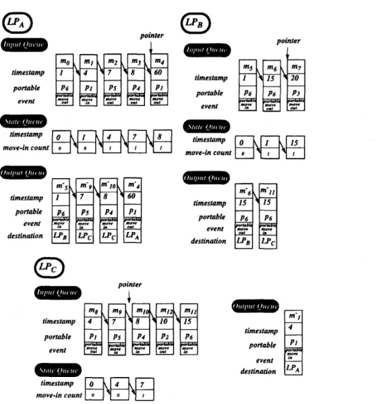
To illustrate the storage reclaimed in fossil collection, consider the example in Fig. 15. In this example, we ignore the phone call events and assume that all Portable-

pointer

c

DO

3

m o w

MoveIn/PortableMoveOut events must be executed in their timestamp order in the optimistic simulation. We further assume that the state variable of a logical process is the number of portables move in the corresponding cell after time 0. Portable 1 moves from cell C to cell A at time 4 and moves from cell A to cell B at time 60. Portable 2 moves from cell C to cell B at time 10. Portable 3 moves from cell B to cell A at time 20. Portable 4 moves from cell A to cell C at time 8. Portable 5 moves from cell A to cell C at time 7. Portable

6 moves from cell A to cell B at time 1 and moves from cell

B to cell C at time 15.

Fig. 16 illustrates the elements in the input/output/state queues of LP.4. L P B , and LPc after all transient messages amve at their destinations, and the GVT value (which is 8 = min(60.20.8)) is found.

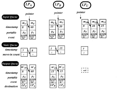
Fig. 17 illustrates the elements in the input/output/state queues of LP.4. LPB, and LPc after the fossil collection procedure is completed.

All messages with timestamps smaller than 8 were fossil collected. Note that fossil collection for

the

state queue

is not

exact the same as that for the input/output queues. In the state queue, the element with the largest timestamp smaller than the GVT value (i.e., 8) must not be removed (see Fig. 17). The other elements with timestamps smaller than 8 are removed. C. Performance Evaluation

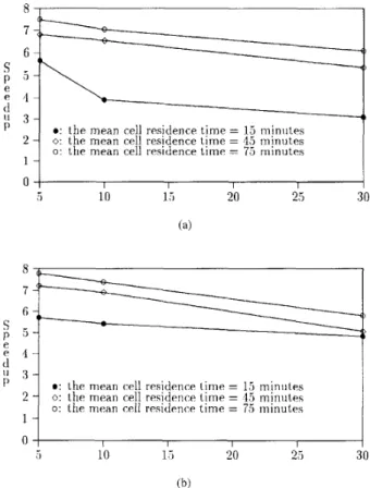
The performance of an optimistic PCS PDES implementa- tion has been investigated in [4]. In this study, a version of

Time Warp has been developed that executes on 8 DEC 5000

workstations connected by an Ethernet.

In the experiments, speedp was used as the output measure where the sequential simulator used the same priority queue