An active control design for a class of parametrically excited systems based on the gradient algorithm

Min-Shin Chen

Ren-Jay Fu

Department of Mectianical Engineering, Nationai Taiwan University, Taipei 106, Taiwan, R.O.C.

An Active Control Design for a

Class of Parametrically Excited

Systems Based on tlie Gradient

Algorithm

This paper introduces a new control design for a dynamic system subject to stationary or nonstationary parametric excitations. In this new design, the system dynamics is transformed into one with a null system matrix using the variation of parameters method. A stabilizing state feedback control can then be immediately obtained by following the gradient algorithm that is originally developed for the parameter identi-fication purpose. Such a design has the advantage that the control requires only past

and present information of the time-varying parametric excitations while previous control designs usually require prediction of future information of the excitations. The closed-loop system stability is guaranteed if the open-loop state response does not diverge too fast. The control design approach can also be applied to the observer design in case where there is only partial observation of the system state.

1 Introduction

A parametrically excited system is one whose state exhibits oscillations or even instability due to internal excitations which appear as time-varying coefficients in the governing differential equation. The phenomena of parametric excitations arise in many branches of physics and engineering. Typical examples in mechanical systems are symmetric satellites in an elliptical orbit (Kane and Barba, 1966), helicopters in forward flight (Webb, Calico and Wiesel, 1991), and pendulums with a verti-cally vibrating support (Nayfeh and Mook, 1979). Parametric excitation can be classified as the stationary excitation and the nonstationary excitation. For stationary excitation, the ampli-tudes and frequencies of the internal excitations (the time-vary-ing coefficients in the governtime-vary-ing equation) are constant. A par-ticular class of such systems are those with periodic parametric excitations. For nonstationary excitation, the amplitudes and frequencies of the internal excitations are time-varying. The analysis of a parametrically excited system conventionally relies on the perturbation method such as the multiple scales approach (Nayfeh and Mook, 1979), which predicts roughly the system stability versus the amplitude of internal excitations. Exact sta-bility analysis is available only when the system is linear and when the excitation is periodically time-varying. In such a case, the Floquet Theory (Callier and Desoer, 1992) can be used to judge the system stability via the locations of n complex

num-bers called the characteristic multipliers.

The active vibration control of systems with periodic para-metric excitations has been studied by several researchers. The most conventional approach is to use the optimal control theory (Kano and Nishimura, 1979, and Bittanti et al. 1986), where the system is stabilized by state feedback control with a periodically time-varying state feedback gain. Calico and Wiesel, 1984, pro-pose an active modal control that can arbitrarily shift the loca-tion of only one characteristic multiplier of the periodic system. Sinha and Joseph, 1994, use the Lyapunov-Floquet transforma-tion to obtain a new system representatransforma-tion with a constant sys-tem matrix. However, their control input is equal to the desired stabilizing control only in the least-squares sense. For linear

systems with nonstationary parametric excitations, the LQ opti-mal control (Kwakemaak and Sivan, 1972) and the controllabil-ity-grammian based control (Rugh, 1993) can suppress the state oscillations effectively. Unfortunately, both control designs im-pose a strict assumption that one must be able to predict how the nonstationary excitations vary in the future in order to calcu-late the desired control input.

In this paper, a new approach to the active control design for parametrically excited systems is presented. The new design utilizes the method of variation of parameters (O'Neal, 1991) to transform the system into one with a zero system matrix (system without drift), and then applies the well-known gradi-ent algorithm in adaptive idgradi-entification (Narendra and Anna-swamy, 1989) to synthesize an active vibration control. Such a design approach, which combines the parameter identification algorithm with the active control design, offers a new perspec-tive on the control design for dynamic systems. The resultant new control can be applied to systems with stationary or nonsta-tionary parametric excitations. Furthermore, there is no need to predict how the parametric excitations vary in the future as long as it is known a priori that the open-loop system response does not diverge too fast.

2 Problem Formulation

Consider a parametrically excited system

x(f) = A ( f ) x ( 0 -f- B ( f ) u ( / ) , x(0) = Xo, y ( 0 = C ( f ) x ( 0 , (1) where \{t) G R" is the system state vector, u ( t ) G R'" is the control input, and y ( 0 ^ R'' is the system output. The system matrix A(f) G R'""', the input matrix B(f) 6 R'""", and the output matrix C ( 0 G R*"^" are time-varying matrices whose elements are (piecewise) continuous. Notice that A ( 0 . B(f) and C(f) are not restricted to be periodical; they can be non-periodical functions of time. It is assumed that given a time interval length T, there exists a positive constant /x such that the state transition matrix (Chen, 1984) *(f, to) G R"*"' of the open-loop system (1) satisfies

Contributed by the Technical Committee on Vibration and Sound for publica-tion in the JOURNAL OF VIBRATION AND ACOUSTICS . Manuscript received Dec.

1995; revised July 1996. Associate Technical Editor; D. T. Mook. where a„

0-max[*(/ + T, t)] ^ IX, \/t> 0, ( 2 )

The number jj, characterizes the open-loop system behavior: the open-loop system is stable, neutrally stable, or possibly unstable depending on whether JJ, < \, fx = \,ot JJL > 1. In this paper, it is assumed that the open-loop system is known to be either stable iix < 1), or neutrally stable (/i = 1), or slightly unstable in the sense that jx is greater than one, but still close to one. When the open-loop system is neutrally stable or slightly unsta-ble due to the parametric excitations in A ( 0 . the control objec-tive is to stabilize the system. When the open-loop system is stable, an active control can become useful if the state conver-gence rate is unsatisfactorily slow. In this case, the control objective is to speed up the state convergence rate of the closed-loop system, and hence to improve the system performance.

Two different cases will be considered in this paper. In the first case, all the state variables x ( ; ) are accessible for measure-ment, and the control objective is to be achieved by a state feedback control

u(f) = - K ( r ) x ( ? ) .

In the second case, only the system output y{t) is accessible for rneasurement. An observer will have to be constructed to estimate the system state x(f), and the control objective is to be achieved by an observer-based state feedback control

u(r) = -K(r)x(r),

where x ( 0 is an estimate of the state x(f) from the observer. For the existence of such stabilizing controls, it is assumed that the system (1) is uniformly controllable as well as uni-formly observable as defined below.

Definition 1 (Chen, 1984): The pair ( A ( 0 , B ( 0 ) is uniformly controllable if there exist A, /?i and P2 ^ R* such that

pJsPM)^p2l, V f > 0 , (3) where Pdt) G R"^" is the controllability grammian defined by

-£

P,(/) A I $ ( r - A, T ) B ( T ) B ' ' ( r ) * ^ ( ; - A, T)dT, in which # ( r , T ) is the open-loop state transition matrix of the system ( 1 ) .

Definition 2 (Chen, 1984): The pair (A(t), C ( 0 ) is uniformly observable if there exist A, 71 and 72 ^ R^ such that

y,I < P „ ( 0 s y^I, \ft > 0, (4) where P o ( 0 G R"^" is the observability grammian defined by

P „ ( 0 4 f $ ' ' ( T , f - A ) C ' ' ( T ) C ( T ) $ ( r , t - A)dT,

Jt-A

in which $ ( ? , T ) is the open-loop state transition matrix of the system ( 1 ) .

3 Gradient Algorithm

The unique feature of this paper is to demonstrate that for a parametrically excited system, the control and observer designs can in fact utilize the gradient algorithm developed for the parameter identification purpose (Narendra and Annaswamy, 1989). Such a "gradient algorithm" design can result in an active control that has several advantages over previous controls (see the following Section).

A brief review of the gradient algorithm will be given below. Let z(?) represents the parameter error between the true parame-ter vector 0 and the estimated parameparame-ter vector © . I f 0 is updated based on the gradient algorithm (Sastry and Bodson, 1989), the governing equation of z(f) is given by

z ( 0 = - 7 w ( 0 w ^ ( 0 z ( 0 , z ( 0 e R", (5)

"regressor vector." A well-known sufficient condition on the exponential stability of the system (5) is that the regressor vector w ( t ) be "persistently exciting" as defined below. Definition 3: The regressor vector w(f) is persistently exciting if there exist positive constants A, a j , and a2 such that

aJ

VI-yv^(T)yv(T)dT s a j l , Vf > 0. (6) The following theorem shows how the parameter error z ( 0 converges to zero under this persistent excitation condition. For completeness of this paper, the proof of the theorem [especially Eq. (7) below, which lays the grounds for the "gradient algo-rithm" design proposed in this paper] is summarized in Appen-dix A.

Tlieorem 1: If the regressor vector w(r) is persistently exciting, the system (5) is exponentially stable in the sense that

\\z(kA)\\

AHO)\\

where

P = J l -

and ai and 0:2 are as in Eq. ( 6 ) . Note that p e (0, 1) for all 7 > 0.

Remaric The parameter error dynamics of the gradient algo-rithm in Eq. (5) is a parametrically excited system that has a very special form for its system matrix A(?) = w(r)w'^(0- The stability result in Theorem 1 thus seems to be very restrictive in terms of the domain of application. However, it will be shown in the following Sections that based on the stability result of this special system ( 5 ) , the control and the observer designs for a general parametrically excited system can be developed quite easily.

4 State Feedback Control Design

The goal of this Section is to find a state feedback gain K(?) such that the following state feedback control

u(f) = - K ( O x ( 0

achieves the control objective mentioned in Section 2. In order to utilize the gradient algorithm introduced in Section 3, the system dynamics (1) has to be transformed into a struc-ture that can match the gradient algorithm in Eq. ( 5 ) . For this purpose, pick a time interval length T, and on each time interval [kT, {k + \)T), apply the following coordinate transformation to the system ( 1 ) :

x ( 0 = * ( r , kT)Zi,(t), t e [kT, (k + l)T),

k = 0,1,2, ... , (8) where z^(t) defines the new state coordinate, and $(f, kT) is the state transition matrix of the open-loop system (1) defined by

d^(t, kT)

dt = A(r)*(f, kT), ^(kT, kT) = I. (9)

where 7 is any positive constant, and w(f) e R" is called the

Notice that on different time intervals, different new coordinates Xt(t)'s, k = 0, 1, . . . are defined. The reason that each new coordinate Zi,(t) is defined only over a finite time interval is that the open-loop state transition matrix # ( r , kT) may ap-proach zero or infinity as time t apap-proaches infinity depending on the open-loop system stability. Hence, the state transforma-tion matrix has to be reset to the identity matrix as shown in Eq. (9) at every time instant t = kT.

According to Eqs. ( 1 ) , (8) and (9), the governing equation of the new state Zic(t) is given by

ik(t) = w,(r)u(r), w,(0 = *(r, kTy'Bit),

t e [kT, (k + l)T), (10) In this new coordinate, the system matrix is identically zero

(the so-called drift-free systems), and this is due to the fact that the open-loop state transition matrix is used as the coordinate transformation matrix. Such an approach, known as the varia-tion of parameter (O'neal, 1991), is commonly used in solving a nonhomogenuous linear differential equation. For a drift-free system, the gradient algorithm in Theorem 1 immediately sug-gests that the control u{t) be chosen as

u(t) = -yMyl(t)z,{t), te[kT,{k+ 1)T), (11) where y can be any positive constant, so that the transformed closed-loop dynamics

i . ( 0 = - y w , ( 0 w j ( 0 z * ( 0 , tG[kT,{k+l)T), (12) has exactly the same structure as the gradient algorithm in Eq. (5) on the time interval [kT, (k + 1)T}.

The following lemma shows that the regressor vector wdt) in Eq. (10) is persistently exciting over the time interval [kT, (k + 1 ) r ) if the system (1) is uniformly controllable.

Lemma 1: If (A(f), B(f)) of the system (1) is uniformly controllable as defined in Eq. ( 3 ) , the regressor vector Wc(0 in Eq. (10) is persistently exciting over the time interval [kT, (k + l ) r ) in the sense that

aj s Pf.(r) = I w,(T)wr(T)rfT s a j / , t e [kT, (k + \)T),

where ai = PJml, and az = fiilm], in which ;0,'s are as in Eq. (3), and mi and m^ are two positive constants satisfying

m i S a , [ * ( / , / f c r ) ] s m 2 , t &[kT,{k + \)T), \/k, (13) in which <b{t,kT)i& defined by Eq. ( 9 ) .

Proof: see Appendix B.

From Eqs. (8) and (11), the proposed control is given by, in terms of the original system state x(r),

u ( 0 = - 7 B ' ' ( f ) * ~ ' a , kT)^^'{t, kT)\(t), y > 0,

t e [kT, (k + l)T). (14) The following theorem states the stability result for the above

control.

Theorem 2: Consider the system (1) and the state feedback control (14). If the system (1) is uniformly controllable, the following results are obtained. (I) The closed-loop system is exponentially stable if the open-loop system is slightly unstable or neutrally stable. (II) The closed-loop system has a faster state convergence rate than the loop system if the open-loop system is stable.

Proof: Without loss of generality, it is assumed that the time interval length T is an integral multiple of A in the definition of Pc(0 in Eq. (3); that is, T = A^A for some positive integer A'. According to Lemma 1 and Eq. (7) in Theorem 1, one can conclude that that, during each time interval [kT, {k + l)T), the norm of the transformed state Zt(t) decays in the following way:

\\z,(kT + T)

p^ihimi

1 - 2yai (1 + yuiVny

From Eq. (8), the transformed state and the original state are related by

\(kT) = ^(kT, kT)z^{kT) = z,(kT), (16) and

x{kT+T) = ^{kT+T,kT)z^{kT+T). (17) Based on Eqs. ( 2 ) , (15), (16) and (17), one can deduce that

\\x{kT + T)\\ ^ lA\z,{kT + T)\\ < lip%z,{kT)\\

= MPllx(fer)||,

and therefore.

\\x{kT)\\ < (Mp")1|x(0)i|, Vfc = 0, 1, 2, (18) When the open-loop system is stable, the number ii,{<\) charterizes the state convergence rate of the open-loop system [ ac-cording to Eq. (2)] while the number/lip" in Eq. (18) character-izes the state convergence rate of the closed-loop system. Since p < 1 by Theorem 1, the effect of the proposed control is to increase the state convergence rate by a factor of p " . Even when the open-loop system is unstable (yu > 1), Equation (18) shows that the closed-loop system can still be stabilized by the proposed control as long as ^u < l/p'^. End of proof.

To determine just what is the maximum p in Eq. (2) allow-able for the chosen control design parameters (y, T), one can proceed as follows. First, calculate the vector Wc(f) according to its definition in Eq. (10), and perform integration to obtain the controllability grammian P c ( 0 in Lemma 1 with A = T. By observing Pc(t) for several time intervals, one can then find out the upper and lower bounds a2 and cci for P ' ( 0 - If the observed upper and lower bounds hold for all time intervals k = 0, 1 , 2 , . . . , [note that it is assumed that the controllability property and the open-loop stability property are uniform with respect to time as suggested by Eqs. (3) and (13)], the maxi-mum allowable p can be estimated according to

Pmax< 1/P~= 1/p = 1 27a, (1 + yaim)' where N = \ since T = A.

In general, there exist no rules in choosing the time interval length T in Eq. ( 8 ) . However, a too large or a too small T is not recommended. If T is chosen too large, and if the open-loop system is unstable, m2 in Eq. (13) will be large. As a result, «! {=pilm\) becomes too small, and this suggests that the controllability of the transformed system (10) is almost lost. If on the contrary T is chosen too small, say, T is close to zero. Pi in Eq. (3) will be small (note that A in Eq. (3) is smaller than T), and m2 in Eq. (13) will be close to one. Hence, a^ ( = P J m \ ) will also become small. In other words, the controlla-bility of the transformed system is almost lost again.

A natural question arises as to whether y can be chosen to maximize the pmax given above so that the proposed control can stabilize an unstable system with a very fast divergence rate. To find the largest p„,ax, or the smallest p possible, one can differentiate p ( 7 ) with respect to y, finding

dp(y)

0 _y" 1 where 0 < p < 1, and

dy ' -Inaj The smallest p is therefore given by

2V« "2

It is seen that the smallest p* is bounded above from zero no matter how the control gain y is chosen, and //max is bounded by 1//9*. This is in fact the main constraint of the gradient algorithm: the convergence rate is limited. As a result, the open-loop response is constrained not to diverge too fast (/Lt can not be too large). Nevertheless, there are other parameter identification algorithms that have a better convergence property than the gradient algorithm. For example, the least-squares algorithm (Sastry and Bodson, 1989) is known to have a much faster convergence rate than the gradient algorithm. The application of the least-squares algorithm to the active control design for parametrically-excited systems is presently under study.

Before concluding this Section, a comparison between the proposed design with other control designs is given below. The

"gradient algorithm" design introduced in this Section has sev-eral important advantages compared with other control designs. In Bittanti et al. (1986), Kano and Nishimura (1979), and Rugh (1993), to obtain the control signal at any time instant t, one must know in advance how the time-varying parameters in A ( 0 and B ( 0 vary in the future. Hence, their controls can be used only when A(/) and B ( 0 are periodically time-varying since prediction of future values of nonstationary time-varying parameters can be extremely difficult is practice. Observe from Eq. (14) that the proposed control relies on the information of ^(t, kT), which depends only on past and present information of the system matrix A ( T ) , r G [kT, t]. Consequently, no future information of the time-varying parameters is needed to calculate the proposed control (14). This characteristics makes the proposed design most suitable for the control of systems with nonperiodical or nonstationary parametric excitations. An-other advantage of the proposed control (14) is that there is no need to take time derivatives of the time-varying parameters in the system matrices A(?) and B(f) as compared with the pole-placement control proposed by Follinger (1978), Wolovich (1968), and Valasek and Olgac (1993). Even though the pole-placement control can be applied to systems with stationary or nonstationary parametric excitations, it requires time derivatives of the time-varying parameters up to the order of the system dimension, which are difficult to measure or identify in practical applications. The control design in this paper avoids this prob-lem since it does not require time derivatives of the time-varying parameters. A by-product of this is that the proposed control can be applied to systems whose time-varying parameters are piecewise continuous in time, while the pole-placement control can only be applied to systems with continuously differentiable time-varying parameters. The third advantage of the proposed control is that when the system has more than one control input, the controllability indices (Chen, 1984) are allowed to change as time evolves, while in the pole-placement control the sys-tem's controllability indices must remain constant (Wolovich, 1968).

5 Observer Design

In this Section, the control objective is to be achieved under a more restrictive condition than in the previous Section: the only accessible signal of the system is the system output y{t) in Eq. ( 1 ) . Under this condition, a state observer will have to be constructed to estimate the system state x(f) from the system output y ( r ) . Consider a conventional Luenberger type observer for the system (1):

k{t) = A(Ox(0 + B(;)u(0 + L(0(y(r) - C{t)x{t)),

x(0) = Xo, (19) where x(/) 6 R" is an estimate of the system state x ( 0 , and L ( ; ) e R"*^'' is the observer feedback gain to be determined

so that x ( 0 approaches x(f) exponentially. Denote the state estimation error by \{t) = x(f) - \i,t). Subtracting Eq. (19) from Eq. (1) yields the state estimation error dynamics

x(/) = [ A ( f ) - L ( O C ( 0 ] S ( r ) . (20) Similar to the control design in Section 4, the observer design will also utilize the gradient algorithm reviewed in Section 3. For this purpose, the following coordinate transformation is introduced for the state estimation error:

x ( 0 = $ ( ? , kTYiM, t e [kT, (k + 1 ) 7 ) ,

fc = 0, 1,2, . . . , (21) where the coordinate transformation matrix <!?(;, kT) is given by Eq. ( 9 ) , and Zt(f) is the new coordinate defined only on the time interval [kT, (k + \)T). From Eqs. (9), (20), and (21), the governing equation of Zj.(r) is given by

z,(r) = -^-\t,kT)Ut)yfl(t)7.{t), Wait) = *''(f, kT)C''(t), t e [kT, (k + l)T). The gradient algorithm in Theorem 1 suggests that the observer feedback gain L(f) be chosen as

L(r) = y^(t,kT)wM),

= y^(t,kT)^''(t,kT)C''(t),

tG [kT,(k + l)T), (22) where y can be any positive constant. The transformed state

estimation error dynamics then becomes

kit) = -yvflit)wM)Ut), t e [kT, (k + l)T), (23) which again has exactly the same structure as the gradient algo-rithm in Eq. ( 5 ) .

The following lemma shows that the uniform observability property of the system (1) guarantees that the regressor vector Wo(f) in Eq. (23) is persistently exciting over the time interval [kT, (k+ 1 ) 7 ) .

Lemma 2: If (A(f), C{t)) of the system (1) is uniformly observable as defined in Eq. (4), the regressor vector w„(0 in Eq. (23) is persistently exciting over the time interval [kT, {k

+ 1 ) 7 ) in the sense that y,m\l^Vl{t)

-I

Proof: See Appendix C.

One can now establish the exponential stability of the state estimation error dynamics (20) for the chosen observer feed-back gain in Eq. (22).

Theorem 3: Consider the state estimation error dynamics (20) and (22). If the system (1) is uniformly observable, the state estimation error X(?) - x{t) converges to zero if the open-loop system is stable, neutrally stable, or slightly unstable in the sense that p, in Eq. (2) is close to one.

Proof: The proof follows exactly that of Theorem 2, and is omitted.

With the proposed observer (19), the state feedback control (14) can now be replaced by an observer-based state feedback control

u ( 0 = -K(t)x{t), (24)

where K(t) is as given in Eq. (14), and x(t) is obtained from the observer (19). By Theorems 2 and 3, and the well-known

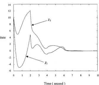
State

Time (second)

Fig. 1 Open-loop state response

Time (second) Fig. 3 Closed-loop state response

Separation Property (Chen, 1984), one can easily show that the closed-loop system state with the control (24) converges to zero exponentially under the hypotheses of Theorems 2 and 3. 6 Simulation Example

Consider the system (1) with nonperiodical parametric exci-tations:

A ( 0 - 1 + 1.5 cos^ it 1 - 1 . 5 sin t cos t - 1 - 1.5 sin r cos f - 1 4 - 1.5 sin^ -Jt

B(r)

4 '

C(t) = [cos {t + sin it 3 cos^ it].

Figure 1 shows the divergent open-loop state response (u(t) = 0). The system is simulated under the proposed observer-based state feedback control (24) with the time interval 7 = 2 seconds, control gain y = 5 in Eq. (14), observer gain 7 = 5 in Eq. (22), and the initial conditions x'"(0) = [10, 10], x ' ( 0 ) = [15, 5 ]. In this simulation, the linear differential equations (1) and (9) are solved by the use of a finite difference approximation with a time step At = 0.01 second. The calculation is done using the MatLab package. Figure 2 shows the time history of

the state estimation error, and Fig. 3 the closed-loop system state; both converging to zero as predicted by Theorems 2 and 3. Figure 4 shows the time history of the control input.

7 Conclusions

In this paper, it is shown that combining the variation of parameter method with the gradient algorithm leads to a new active control design for parametrically excited systems. The new design has an important advantage that only past and pres-ent information of the time-varying parametric excitations is required to calculate the control input, while previous designs usually require future information. However, the new control has a constraint that the open-loop system response can not diverge too fast, and this is mainly due to the fact that the gradient algorithm has a limited convergence rate. Research is currently being conducted to explore the possibility of em-ploying various different parameter identification algorithms such as the least-squares algorithm in the active control design in order to overcome this constraint.

Acknowledgment

The work in this paper is supported by the National Science Council of the Republic of China under grant no. NSC 85-2212-E-002-001. State Estimation -2 Errors -4 0 1 2 3 4 5 6 7 8 Time (second)

Fig. 2 State estimation error of the observer

Control

2 3 4 5 6

Time (second)

Fig. 4 Control input

References

Bittanti, S., Colaneri, P., and Guardabassi, G., 1986, "Analysis of the Periodic Lyapunov and Riccatic Equations via Canonical Decomposition," SIAM. J.

Con-trol and Optimization, Vol. 24, pp. 1138-1149.

Calico, R. A., and Wiesel, W. E., 1984, "Control of Time-Periodic Systems,"

j . of Guidance, Vol. 7, pp. 671-676.

Callier, F., and Desoer, C. A., 1992, Linear System Theory, Springer-Verlag, Hong Kong.

Clien, C. T., 1984, Linear System Theory and Design, Holt, Rinehart and Win-ston, New Yorlt.

Follinger, O., 1978, "Design of Time-Varying Systems by Pole Assignment,"

Regelungstechink, Vol. 26, pp. 85-95.

Kane, T. R., and Bara, P. M., 1966, "Attitude Stability of a Spinning Satellite in an Elliptical Orbit," ASME Journal of Applied Mechanics, Vol. 33, pp. 4 0 2 -405.

Kano, H., and Nishimura, T., 1979, "Periodic Solutions of Matrix Riccati Equations with Detectability and StabiUzabiiity," Int. J. Control, Vol. 29, pp. 471-487.

Kwakernaak, H., and Sivan, R., 1972, Linear Optimal Control Systems, Wiley, New York.

Narendra, K. S., and Annaswamy, A. M., 1989, Stable Adaptive Systems, Pren-tice-Hall, Englewood CUffs, New Jersey.

Nayfeh, A. H., and Mook, D. T., 1979, Nonlinear Oscillations, Wiley-Intersci-ence. New York.

O'Neil, P. v., 1991, Advanced Engineering Mathematics, Wadsworth, New York.

Rugh, W. J., 1993, Linear System Theory, Prentice-Hall, Englewood Cliffs, New Jersey.

Sastry, S., and Bodson, M., 1989, Adaptive Control, Stability, Convergence,

and Robustness, Prentice-Hall, New York.

Sinha, S. C , and Joseph, P., 1994, "Control of General Dynamic Systems with Periodic Varying Parameters via Lyapunov-Floquet Transformation," ASME

Journal of Dynamic Systems, Measurement, and Control, Vol. 116, pp. 650-658.

Valasek, M., and Olgac, O., 1993, "GeneraUzation of Ackermann's Formula for Linear MIMO Time-Invariant and Time-Varying Systems," Proceedings of

Conference on Decision and Control, pp. 827-831.

Webb, S. G., Calico, R. A., and Wiesel, W. E., 1991, "Time-Periodic Control of a Multiblade Helicopter," J. of Guidance, Vol. 14, pp. 1301-1308.

Wolovich, W. A., 1968, "On the Stabihzation of Controllable Systems," IEEE

Trans, on Automatic Control, Vol. 13, pp. 569-572. A P P E N D I X A

First, note that the persistent excitation condition on w(f) in Eq. (6) is equivalent to the fact that the pair (0, w^(r)) is uniformly observable with its observability grammian satisfying the inequalities in Eq. ( 6 ) . Quoting Lemma 2.5.2 and Theorem 2.5.1 in Sastry and Bodson (1989), one can conclude that the pair ( - 7 w ( 0 w ^ ( 0 , w'^(f)) is also uniformly observable with its observability grammian satisfying the inequality

(1 -I- yaj^f I ^ P . ( 0 . ( A l ) • Second, choose a Lyapunov function candidate for the system (5): V(?) = z'^it)z(t) = ||z(r)f. Calculating the time deriva-tive of V ( 0 yields

V = 2 z ' ' ( r ) z ( 0

= -2yz'^{t)wit)w''(t)zit). Integrating the above equation from f - A to f gives

\Ht) r-\\z{t-A)f

z''(T)w(r)w''(T)z(r)rfT. (A2)

Let the state transition matrix of the system (5) be *(f, T ) , then

Z ( T ) = * ( T , t - A ) z ( r - A ) .

Substituting the above relationship into Eq. (A2) results in

||z(Of - Mt - A)f

||z(Of ^ p'Mt - A ) f , V? > 0, where

0 < p ' = 1 - 2yai

(I + ya2yn) < 1, Vy > 0. (A3) Equation (A3) suggests that z(t) converges to zero as indicated by Eq. ( 7 ) . End of proof.

A P P E N D I X B

Notice that Vl(t) in Lemma 1 is the controllability grammian of the pair (0, w^.(r)), and it is related to the system's controlla-bility grammian PdO in Eq. (3) by

Pl(t) = #(/tr, t - A)P,(o*''(fcr, t - A). (Bi)

Given any constant vector x, one has

Pi\\^''(kT, t - A)xf =a x ^ J ( O x s l32WikT, t - A ) x f , due to Eq. ( 3 ) . Since ^{kT, r - A) = ^-\t - A, kT), it follows from Eq. (13) that

Therefore,

^ < WikT, t - A)x|| < ^ .

m2 Wi

4 ||x|r ^ xT>KOx s ^ llxf,

m5 m^ and this verified the claim of Lemma 1. End of proof.

A P P E N D I X C

The proof of Lemma 2 duplicates that of Lemma 1, except that Eq. ( B l ) is now replaced by