The Effect of Flow Velocity on Microcantilever-Based Biosensors

THE EFFECT OF FLOW VELOCITY ON

MICROCANTILEVER-BASED BIOSENSORS

M.-C. Wu * _{J.-S. Chang} ** _{K.-C. Wu} ** _{C.-H. Lin} * _{C.-Y. Wu} ***

Institute of Applied Mechanics National Taiwan University Taipei, Taiwan 10617, R.O.C.

ABSTRACT

This work focuses on studying the effect of flow velocity on microcantilever-based biosensor by nu-merical simulation. The microcantilever sensors used in detecting biomolecules have attractive advan-tages like cost efficiency, real-time and ability of fabricating in array. Both rectangular and triangular shapes of a general model of microcantilever beam are considered. Several important physical phenom-ena are obtained. Comparing with the first order Langmuir theory, we have calculated the effect on the reactive rate, produced concentration, the distribution of concentration and deflection in the z axis by solv-ing these physical coupled problem involvsolv-ing flow field, concentration field and chemical reaction on the reaction surface. It is found numerically that the transportation of analyte, reactive rate, the distribution of concentration and deflection in the z axis are all effected by changing the flow velocity. The result has shown that flow velocity is an important factor for this biosensor.

Keywords : Microcantilever, Biosensor, Finite element method.

1. INTRODUCTION

With the advanced in nanotechnology in recent year, biosensor is widely used to detect small biomolecules and biosensing applications have been moving toward fast. Biosensor technology is a powerful analytical technique in biological systems for its small and low- cost characteristic. Combining with chemical or physical transducer, biosensors use antibodies or other kinds of biomolecules for molecular recognition. Bio-molecular recognition is a natural characteristic of the human body and many kinds of life. It has some advantages like highly sensitive, real-time, label-free and quantitative analysis on biomolecular recognition. Commonly biosensors are used as the microcantilever sensor, surface plasma resonance (SPR) and quartz crystal microbalance (QCM). These are three methods which are mostly used to detect small molecules.

Microcantilever has been proposed as mechanical transducer for recent years [1~3]. The original appli-cation comes from atomic force microscope (AFM). It is fabricated of silicon nitride and coated a gold layer to link up the specific self-assembly molecules [4~5]. The variation of the surface stress due to the combina-tion of analytes and ligands results in the defleccombina-tion of the cantilever beam [6]. Therefore, the biomolecular recognition can be translated into nanomechanical mo-tion by using physical transducer, and then the quantita-tive detection of biomolecule in the solid and liquid

interfaces could be obtained. Microcantilever sensors offer a platform for the label-free analysis of protein- protein interaction, enzyme reaction, and DNA hybridi-zation [7~8].

These biosensors are usually put in the flow field to detect biomolecule and can satisfy miniaturization. The adsorption of analyte depends on two processes: mass transportation process and chemical reaction process. Langmuir et al. [9] brought up the first order Langmuir theory presenting the reaction model for an-tibody and antigen in the solid and liquid interfaces; Illkonic et al. [10] developed the pure diffusion- controlled model; Rahn et al. [11] proposed the diffu-sion limited Langmuir model; Nicholas et al. [12] had proved that under low concentration and low flow ve-locity, the thickness of diffusion layer will have effect on reaction rate. Therefore flow velocity will be an important factor for the development of thickness of diffusion layer.

In this work, we present a model for the microcanti-lever sensor relationship to establish the effect by flow velocity and to derive the relation of reactive rate, pro-duced concentration, the distribution of concentration and deflection in the z axis. The finite element nu-merical simulation was built and set up on COMSOL Muityphysics. Comparing with different flow veloci-ties, the results have shown that faster flow velocity will get more remarkable effects.

2. MATHEMATICAL MODEL

In the solid-liquid interface, the reaction has two step events:

Mass transportation process: The analyte is trans-ferred out of the bulk solution towards the reaction sur-face.

[ ]Abulk R [ ]Asurface (1) Chemical reaction process: The binding of the analyte to

the ligand take place.

[ ] [ ] a [ ] d K surface K A + B R AB (2)

where [A]bulk is the analyte in the bulk, [A]surface is the analyte on the gold surface with ligand bound to the dextran matrix, [B] is the ligand , [AB] is the analyte- ligand complex, Ka is the association rate constant, and

Kd is the dissociation rate constant.

2.1 Governing Equations of the Flow Field

We assume that the density ρ and viscosity η of the modeled fluid are constant, that is, they are not affected by temperature and concentration. The governing equations of continuity and three-dimensional momen-tum can be expressed as follows:

0 V ∇ ⋅ =JG (3) 2 ₀ u _{V u u} p t x ∂ ∂ ρ + ρ ⋅∇ − η∇ + = ∂ ∂ JG (4) 2 ₀ v _{V v v} p t y ∂ ∂ ρ + ρ ⋅∇ − η∇ + = ∂ ∂ JG (5) 2 ₀ w p V w w t z ∂ ∂ ρ + ρ ⋅∇ − η∇ + = ∂ ∂ JG (6) where u, v, w are the velocity components in the x, y, z

directions, respectively; η is dynamic viscosity of the fluid; ρ is density of the fluid; p is the pressure.

No-slip boundary conditions are assumed between the inter faces of the microcantilever and the flow. A total load FK from the flow, consisting of a pressure component and a viscous drag component, is applied to the boundary of this structure. This load, defined as force per area, equals:

( ( ( ) ))T

FK= ⋅ − + η ∇ + ∇nK pI uK uK (7)

where p is the fluid pressure; I is the unit tensor; η is the dynamic viscosity; uK is the velocity field; nK is the normal unit vector of the boundary pointing out from the fluid. If this load is not small, negligible distur-bance will be produced during the measurement of de-flection of the microcantilever due to surface stress.

2.2 Governing Equations of Concentration Field

Transportation of the protein from the flow to the surface is caused by fluid flow and diffusion. In order to solve the problem, we apply Fick's Second Law.

2 2 2 2 2 2 [ ] [ ] [ ] [ ] [ ] [ ] [ ] A A A A u v w t x y z A A A D x y z ∂ ₊ ∂ ₊ ∂ ₊ ∂ ∂ ∂ ∂ ∂ ⎛∂ ∂ ∂ ⎞ = ⎜ _∂ + _∂ + _∂ ⎟ ⎝ ⎠ (8)

where [A] is the concentration of analyte; and D is the diffusion coefficient.

2.3 Governing Equations of Reaction Surface

The reaction between an immobilized ligand and analyte can be assumed to follow the first order Lang-muir adsorption model. During the association phase, the complex [AB] increases as a function of time ac-cording to：

{

}

The relation between concentration gradients on the surface and the rate of reaction is given by

{

}

where [A]surface is the analyte at the gold surface with ligand bounded to the dextran matrix; [B] is the ligand, [AB] is the analyte-ligand complex; Ka is the association rate constant; and Kd is the dissociation rate constant.

3. SIMULATION AND RESULTS

Simulation and modeling for microcantilever sensor are conducted using COMSOL Muityphysics. The microcantilever is fabricated by silicon nitride and takes the size as 230µm in length, 40µm in width and 3µm in thickness for rectangular microcantilever, take the size as 200µm in height, 40µm in each leg and form with 45 degree for triangular microcantilever. The size of flow chamber is 500µm in width and length, 100µm in height. The material parameters are listed on the Table. 1.

3.1 The Difference Between the First Order Langmuir Theory and Simulation

This simulation takes more time to allow the results to reach the steady state than the first order Langmuir adsorption theory does. [A]surface is not equal to [A]bulk until the reaction is over. The absorption limitation in this simulation means that the diffusion is too slow for the analyte to reach the reactive surface and can not chemically reacted with the ligand when the flow veloc-ity is too slow, the diffusion coefficient is small and ka is

Table 1 Parameters of FEM simulation

Property Value

Young’s Modulus of SiN 150 GPa

Poisson ratio of SiN υ 0.23

Density of SiN 2330kg/m3

Mass damping parameter 1 1/s

Stiffness damping parameter 0.001s

Flow density ρ 1 × 103_kg/m3

Diffusion coefficient 1 × 10−10_m2_/s

Association rate constant Ka 2000M−1S−1

Dissociation rate constant Kd 0.001S−1

Concentration of [A]bulk 1 × 10−5_M

Concentration of [B] 1 × 10−8_mole/m2

Dynamic viscosity η 1 × 10−3 _Pa⋅S

high. From Fig.1 we know that [A]surface will reach [A]bulk soon when the flow velocity is 1e-1 (m/s) unless the speed of rate of absorption is greater than the speed of rate of [A]bulk initially. The concentration is closer to the first order Langmuir theory as the flow velocity is faster. As the ligand combines with analyte, the trends of this simulation shown in Fig. 2 is approximately the same as that shown in Fig. 1. It takes more time to reach the steady state than the first order Langmuir ad-sorption theory does.

3.2 The Effect of Different Flow Velocity on Reactive Rate and Time for Steady State

We compare the reactive rates for the two different shapes of microcantilevers with different inlet velocities (1e-4, 1e-3, 1e-2, 1e-1m/s). The result for steady state is listed on the Table 2. From the table we know that the faster the flow velocity, the faster the concentration to reach the steady state. From the reactive rates we know that the slower the flow velocity, the longer the time to reach the fastest reactive rate by mass transport process, and the fastest reactive rate for low velocity is much lower than that for the high flow velocity as Figs. 3 and 4. Since the produced concentration on left side of the triangular microcantilever is higher than that on the right side and the concentration is not uniform, the reactive rate is slower than the rectangular one as Fig. 5.

3.3 The Effect of Different Flow Velocity for Produced Concentration Distribution

From Figs. 6 and 7 it can be seen that the slower the flow, the thicker the thickness of the diffusion layer. The trend is described as the equation

1 1 6 3 x D v u δ =

which is derived from Jung et al [13], where δ is the thickness of the diffusion layer; D is the diffusion coeffi-cient; v is Kinematic viscosity; u is the flow velocity in x direction; x is the position from the reactive surface where we get the data point. Figure. 8 shows the con-centration distribution profile of [A] for rectangular mi-crocantilever.

0 100 200 300 400 500 600 0.0 2.0x10-6 4.0x10-6 6.0x10-6 8.0x10-6 1.0x10-5 [A ] (m ol e/ m 3) time(s) velocity 1e-1(m/s) velocity 1e-2(m/s) velocity 1e-3(m/s) velocity 1e-4(m/s) first order langmuir

Fig. 1 [A]surface vs. time in different flow velocity with the first Langmuir theory

0 100 200 300 400 500 600 0.0 1.0x10-9 2.0x10-9 3.0x10-9 4.0x10-9 5.0x10-9 6.0x10-9 7.0x10-9 8.0x10-9 9.0x10-9 1.0x10-8 [A B]( m ole /m 2) time(s) velocity 1e-1(m/s) velocity 1e-2(m/s) velocity 1e-3(m/s) velocity 1e-4(m/s) first order langmuir

Fig. 2 [AB] vs. time in different flow velocity with Langmuir Theory 0 50 100 150 200 250 300 350 400 450 500 550 600 0.0 5.0x10-11 1.0x10-10 1.5x10-10 2.0x10-10 rea ctive ra te time(s) velocity 1e-1(m /s) velocity 1e-2(m /s) velocity 1e-3(m /s) velocity 1e-4(m /s)

Fig. 3 Reactive rate vs. time for rectangular microcantilever 0 50 100 150 200 250 300 350 400 450 500 550 600 0.0 5.0x10-11 1.0x10-10 1.5x10-10 2.0x10-10 r eac tiv e r a te time(s) velocity 1e-1(m /s) velocity 1e-2(m /s) velocity 1e-3(m /s) velocity 1e-4(m /s)

Fig. 4 Reactive rate vs. time for triangular microcantilever

Table 2 Time reguired to reach steady state for dif-ferent shapes of microcantilevers under vari-ous flow velocities

Velocity (m/s) 1e-1 1e-2 1e-3 1e-4

rectangular (s) 320 320 345 590 triangle (s) 380 380 405 640 0 50 100 150 200 250 300 350 400 450 500 550 600 0.0 1.0x10-11 2.0x10-11 3.0x10-11 4.0x10-11 5.0x10-11 6.0x10-11 7.0x10-11 re a ct ive r a te time(s)

velocity of triangular microcantilever 1e-4(m/s) velocity of rectangular microcantilever 1e-4(m/s)

Fig. 5 Reactive rates for triangular and rectangular microcantilever at flow speed 1 × 10−4 _(m/s)

Fig. 6 The distribution of concentration for flow velocity 1 × 10−4 _(m/s)

Fig. 7 The distribution of concentration for flow velocity 1 × 10−2 _(m/s)

Fig. 8 The concentration distribution on rectangular microcantilever for flow velocity 1 × 10−4 _(m/s)

of [AB] on the surface is plotted on the Figs. 9 and 10. We use the cutting line to observe the concentration distribution on the surface as Fig. 11. The concentra-tion which is near the inlet is a little higher. The cov-erage rate will differ by 20% at the same time (60sec) with flow velocity 1e-4 (m/s) on the surface of microcantilever with width of 40µm as plotted on Figs. 12 and 13. Because the two sides of the reactive surface are closer to the fluid, the concentrations at the edges comparing to that at the central place will be higher. Figures 14 and 15 reveal coverage with vary-ing time.

Fig. 9 The produced concentration distribution of [AB] for triangular microcantilever

Fig. 10 The produced concentration distribution of [AB] for triangular microcantilever

y=100μm x=250μm

y=100μm x=250μm

Fig. 11 The two cutting line for microcantilever (x = 250 × 10−6_{m y = 100 × 10}−6_m)

0.00000 0.00001 0.00002 0.00003 0.00004 0.30 0.32 0.34 0.36 0.38 0.40 0.42 0.44 0.46 0.48 0.50 0.52 0.54 0.56 0.58 0.60 0.62 co ver ag e microcantilever width velocity 1e-1(m/s) velocity 1e-2(m/s) velocity 1e-3(m/s) velocity 1e-4(m/s)

Fig. 12 (y = 100 × 10−6_{m) rectangular microcantilever}

width coverage vs. after 60 seconds of opera-tion 0.00000 0.00005 0.00010 0.00015 0.00020 0.2 0.3 0.4 0.5 0.6 cover age microcantilever width velocity 1e-1(m/s) velocity 1e-2(m/s) velocity 1e-3(m/s) velocity 1e-4(m/s)

Fig. 13 (x = 250 × 10−6_{m) rectangular microcantilever}

width coverage vs. after 60 seconds of opera-tion 0.0 1.0x10-5 _2.0x10-5 _3.0x10-5 _4.0x10-5 0.0 0.2 0.4 0.6 0.8 1.0 cov er age microcantilever width time=0 time=100 time=200 time=400 time=600

Fig. 14 (y = 100 × 10−6_{m) rectangular microcantilever}

width coverage vs. with time varying changing with flow velocity 1e-4

0.0 5.0x10-5 _1.0x10-4 _1.5x10-4 _2.0x10-4 0.0 0.2 0.4 0.6 0.8 1.0 cov erage microcantilever length time=0 time=100 time=200 time=400 time=600

Fig. 15 (x = 250 × 10−6_{m) rectangular microcantilever}

width coverage vs. with time varying changing with flow velocity 1 × 10−4

3.4 Deflection Analysis for Microcantilever in Dif-ferent Flow Velocity

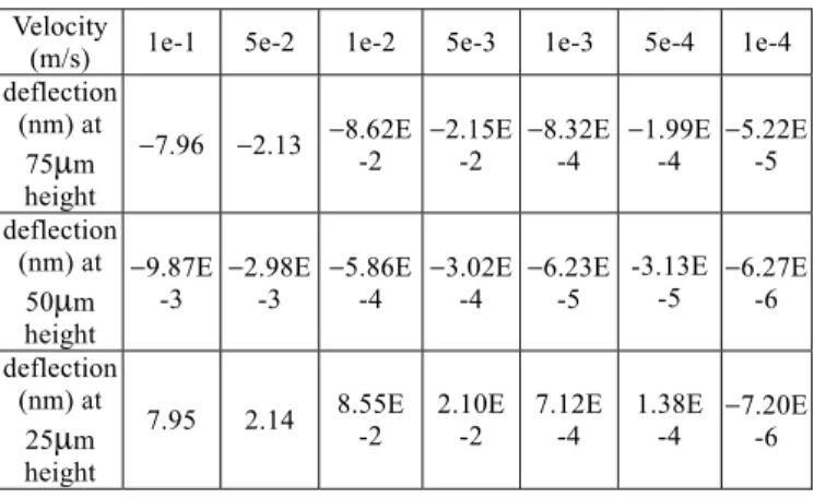
We simulate triangular and rectangular microcantile-vers at different place in three dimension flow tunnel as Figs. 16 and 17 and compare different inlet flow veloc-ity 1e-4, 1e-3, 1e-2, 1e-1 (m/s) which has effect on de-flection by shear force and pressure distribution. The force can be described as the Eq. (2)~(7). The deflec-tions of these two kinds of microcantilever at three po-sitions (75µm, 50µm, 25µm from the bottom) are listed in Tables 3 and 4. Theoretically the deflection of mi-crocantilever placed in different places should be the same, but actually it will be a little different by mesh grid which we use. The microcantilever should be put in its central place (in the z-direction) to avoid the disturbance of deflection from the flow field. It may produce an 8 ~ 10 (nm) deflection at flow velocity 1e-1 (m/s) when the microcantilever is put at the position 75(µm) or 25(µm) in the z-direction.

Fig. 16 The deformation of rectangular microcantilever

Fig. 17 The deformation of triangular microcantilever Table 3 Deflection of the triangle microcantilever due

to velocity effects Velocity

(m/s) 1e-1 5e-2 1e-2 5e-3 1e-3 5e-4 1e-4 deflection

(nm) at 75µm height

−1.01E1 −2.45 −6.25E _-2 −4.54E _-3 3.38E _-3 1.96 E_-3 4.34E_-4 deflection

(nm) at 50µm height

2.32E

-2 4.35E-3 1.20E -3 6.59E -4 1.43E -4 7.22E-5 1.46E-5 deflection

(nm) at 25µm height

Table 4 Deflection of the rectangle microcantilever due to velocity effects

Velocity

(m/s) 1e-1 5e-2 1e-2 5e-3 1e-3 5e-4 1e-4 deflection

(nm) at 75µm height

−7.96 −2.13 −8.62E_-2 −2.15E _-2 −8.32E _-4 −1.99E_-4 −5.22E_-5 deflection

(nm) at 50µm height

−9.87E

-3 −2.98E -3 −5.86E-4 −3.02E -4 −6.23E -5 -3.13E -5 −6.27E-6 deflection (nm) at 25µm height

7.95 2.14 8.55E _-2 2.10E _-2 7.12E _-4 1.38E_-4 −7.20E_-6

4. CONCLUSIONS

A simple microcantilever model has been set up to simulate physical phenomenon in three dimensional flow field. We get some important conclusions: 1. The concentration of [AB] complex will be close to

that given by the first order Langmuir theory when the flow velocity is high.

2. The faster the flow velocity, the faster the reactive rate to reach the steady state.

3. Compared the inner part of the reactive surface, the leading and the trail sides have high concentrations of [AB] complex.

4. The faster the flow velocity will induce a larger de-flection in the z-axis, and the microcantilever should be put in a central place to avoid the disturbance of deflection from the flow field.

ACKNOWLEDGEMENTS

This research is supported by the National Science Coun-cil in Taiwan through Grant NSC 94-2120-M-002-014.

REFERENCES

1. Battiston, F. M., Ramseyer, J. P., Lang, H. P., Baller, M. K., Gerber, Ch., Gimzewski, J. K., Meyer, E. and Guntherodt, H. J., “A Chemical Sensor Based on a Microfabricated Cantilever Ar-ray With Simultaneous Resonance-Frequency and Bending Readout,” Sensor and Actuators B, 77, pp. 122−131 (2001).

2. Yoo, K. A., Na, K. H., Joung, S. R., Nahm, B. H., Kang, C. J. and Kim, Y. S., “Microcantilever-Based Biosensor for Detection of Various Biomolecules,”

Japanese Journal of Applied Physics, 45, 1B, pp.

515−518 (2006).

3. Moulin, A. M., O’Shea, S. J. and Welland, M. E., “Microcantilever-Based Biosensors,”

Ultramicro-scopy, 82, pp. 23−31 (2000).

4. Berger, R., Delamarche, E., Lang, H. P., Gerber, C., Gimzewski, J. K., Meyer, E. and Güntherodt, H. J., “Surface Stress in the Self-Assembly of Al-kanethiols on Glod,” SCIENCE, 276, pp. 2021− 2024 (1997).

5. Poirier, G. E. and Pylant, E. D., “The Self- Assembly Mechanism of Alkanethiols on Au(111),” Science, New Series, 272(5265), pp. 1145−1148 (1996).

6. Raiteri, R., Butt, H. J. and Grattarola, M., “Changes in Surface Stress at Liquid/Solid Interface Meas-ured with a Microcantilever,” Electrochimica Acta, 46, pp. 157−163 (2000).

7. Wu, G., Datar, R. H., Hansen, K. M., Thundat, T., Cote, R. J. and Majumdar, A., “Bioassay of Pros-tate-Specific Antigen (PSA) Using Micro- cantilevers,” Nature Biotechnology, 19, pp. 856− 860 (2001).

8. Wu, G., Ji, H., Hansen, K., Thundat, T., Datar, R., Cote, R., Hagan, M. F., Chakraborty, A. K. and Majumdar, A., “Origin of Nanomechanical Canti-lever Motion Generated from Biomolecular Inter-actions,” Proceedings of the National Academy of

Sciences of the United States of America 98, pp.

1560−1564 (2001).

9. Langmuir, I., “The Adsorption of Gases on Plane Surfaces of Glass, Mica and Platinum,” J. Am.

Chem. Soc., 40, pp. 1361−1403 (1918).

10. Ilkovic, D., Collect. Czech. Chem. Commun., 6, p. 498 (1934)

11. Rahn, J. R. and Hallock, R. B., “Antibody Binding to Antigen-Coated Substrates Studied with Surface Plasmon Oscillations,” Langmuir, 11, pp. 650−654 (1995).

12. Nicholas Camillone, “Diffusion-Limited Thiol Ad-sorption on the Gold(111) Surface,” Langmuir, 20, pp. 1199−1206 (2004).

13. Jung, L. S. and Campbell, C. T., “Sticking Prob-abilities in Adsorption of Alkylthiols from Liquid Ethanol Solution onto Gold,” J. Phys. Chem. B, 104, pp. 11168−1117 (2000).

(Manuscript received November 16, 2006, accepted for publication February 15, 2007.)