Multiple Objective Planning for Production and Distribution Model of Supply
Chain: Case of Bicycle Manufacturer
Gwo-Hshiung Tzeng, Yu-Min Hung and Min-Lan Chang
Institute of Technology Management, Institute of Trafic and TransportationCollege of Management, National Chiao Tung University 1001, Ta-Hsuch Rd., Hsinchu 300, Taiwan
ghtzeng@cc.nctu.edu.tw
Abstract
Under increasing globalization, enterprises view supply chains (SC) as an integration of process control and management. The bicycle industry is one of the competitive industries in Taiwan, for which there is a complete supply chain system. To internationalize and improve the competitive advantage of this industry, it is necessary for it to improve the capacity of global production and distribution. In this paper, we consider both the maximum profit of enterprises and the maximum quality of customer service, using five programming methods to construct multi-objective production and distribution models. These five methods are: compromise programming, fuzzy multi-objective programming, weighted multi-objective programming, weighted fuzzy multi-objective programming and two-phase fuzzy multi-objective programming. The results reveal that the weighted multi-objective model was better for considering the maximum profit of enterprises and the maximum quality of customer service. Finally, we use the weighted multi-objective model for sensitivity analysis. These results show that after raising the per-unit production cost in production processes, the total profit would decrease. In addition, if the unit inventory cost increases due to improving the customer service level, then the total profit might increase, but not significantly. Furthermore, the shortage cost seems have interactive behavior on the enterprises, in which an increase of inventory cost will lower shortage cost.
Keywords: supply chain, bicycle industry, fuzzy
multi-objective programming
1. Introduction
Due to the trend of globalization, the supply chain is increasingly important for many enterprises as one of the flow process controls and levels of management to be integrated. Ranging from the supply of raw materials, production, distribution, retail sales, and after-sales service to consumers, the primary objectives are to lower the total costs of production along the supply chain, and to increase production efficiency. With positive efforts from both government and industry, Taiwan has been admitted into the World Trade Organization (WTO) on January 1, 2001. Within the context of WTO, manufacturers are confronted with global competition, the need to accelerate the flow of materials and information. As a result, the development of
an effective supply chain is essential for an industry to become successful.
The bicycle industry, generally considered as conventional industry, demands massive labor capital investment. With its development over the last fifty years, the industry supply chain has complete up-, middle-, and down-stream manufacturers, making Taiwan one of the significant bicycle manufacturing centers of the world. In 1980, the amount of bicycles sold overseas ranked first world-wide, surpassing that of Japan. Nevertheless, although bicycles are not a high-tech product they do follow trends of fashion, creativity and diversity of product, go speed of supply has become critical to compete in the face of saturated markets, supply greater than demand, and the diversified demands of consumers. Therefore, this study aims to strengthen the capabilities of global management, to expand the core system of this industry into a global supply and demand chain, to provide timely production and high service quality, enhancing the competitiveness of these on the international market.
As Taiwan’s bicycle industry is exposed to international competition, bicycle manufacturers must develop global management abilities to confront this new situation. As a result, this study considers multiple objective production and distribution, focusing on Taiwan’s conventional bicycle manufacturing industry, considering enterprise profit and customer service level for multi-objective programming to develop a production and distribution model for bicycle manufacturers in Taiwan.
Here, five multi-objective programming methods have been adopted for comparison: multi-objective compromise programming, fuzzy multi-objective programming, weighted multi-objective programming, weighted fuzzy multi-objective programming, and two-phase fuzzy multi-objective programming. These five methods have used to compare in resolution for this model. Finally, weighted multi-objective programming has been used to conduct sensitivity analysis in order to obtain outcomes that manufacturers can use for reference in developing their supply chains. The results show that when increasing the per unit production cost in production processes, the total profit would decrease. If the unit inventory cost increase for improving the service level of customer, the total profit might increase, but not significantly. Furthermore, shortage cost seems have an
The Second International Conference on Electronic Business The Second International Conference on Electronic Business
interactive behavior on the enterprises, and increased inventory cost will lower the shortage cost.
The remainder of this paper is organized as follows. In Section 2 previous literature is presented. In Section 3 a model for the bicycle supply chain is established. In Section 4 an example for applying this model to the bicycle supply chain is presented. Finally conclusions and recommendations are provided.
2. Previous Literature on Supply Chain and
Multi-objective Programming for Production
and Distribution
Since this study explores the issues of production and distribution of bicycle manufacturing, which is related to management operation and industrial supply chain, we first review previous literature on supply chain management. Then, we present studies on multi-objective programming, compromise programming, fuzzy multi-objective programming, weighted multi-objective programming, and two-phase fuzzy multi-objective programming, since they are issues of production and distribution of bicycle manufacturing.
2.1 Relevant literatures of supply chain
Chandra and Fisher (1994) dealt with the production and delivery of a single factory with single production in multiple periods. Comparing the separation and integration models of production and transportation problems, they found that the integration model of production and delivery can help to lower total costs. Nagata et al. (1995) examined the production and transportation problems of multiple products and multiple factories in multiple periods, using multi-objective and fuzzy multi-objective model for programming. There the programming problem for multiple periods included obtaining uncertain information when considering a management plan so as to construct a reasonable multi-objective production and transportation model. Tzeng et al. (1996) addressed the needs of practical issues, using fuzzy bi-criteria multi-index linear programming to deal with uncertain supply and demand environments in face of the coal procurement and delivery schedule for the Taiwan Power Company (TPC). This kind of problem has multiple destinations, multiple kinds of goals, and multiple kinds of shipping vessels. Petrovic et al (1998, 1999), used fuzzy models and simulation for the supply chain, and developed a decision-making system for an uncertain environment. Thus, they determined the inventory level and the order amounts with the supply chain model to simulate operation control with limited time and reasonable cost. Van Der Vorst et al. (1998) considered that supply chain management should include lowering or limiting uncertainty, so that the integral benefits of the supply chain could be improved. Sources of uncertainty include the following: vertical order prediction, information input, administration management, decision-making procedures, and innate uncertainty. This study used the food chain as example to improve the structure of allocation and operation management.
Although many factors of uncertainty were eliminated in that illustration, results indicated that the reasonable benefit of supply chain management has also been determined. Dhaenens-Flipo (2000) proposed clustering problems of production and transportation of multiple products from multiple factories for integrated programming. To deal with sophisticated problems with spatial decomposition he changed them into sub-problems, and employed the resolution method for vehicle routing problem (VRP), which also helped simplify the problem and lower total costs.
To sum up, when this current study considers the maximization of both enterprise profit and customer service level, the resolution can also be obtained from developing a multi-objective programming model in view of global supply chain system. The proposed model is described in the following section.
2.2 Multi-objective and fuzzy multi-objective programming
Zeleny (1982) pointed out that there is nothing about decision making in programming when there is only one single objective, as decision making is already endowed in the estimation of the objective function value coefficient. Thus, when the objective function coefficient is determined the decision maker can only accept or discard the outcome resolved by the model, and no other information can ever be obtained from the model by the decision maker. As can be seen, the development of “multi-objective programming” was brought about by the incomplete consideration taking account of only one single objective, as well as the fact that the decision maker can either accept or discard the optimal solution presented. In contrast, the objective of multi-objective programming is mainly to find a feasible non-inferior solution set or compromise solution so that the decision maker can effectively focus on the trade-offs when several objectives are in conflict. This is generally indicated as follows:
1 2 [ ( ), ( ),..., ( )] . . k max/min = f f f s t ≤ ≥ f x x x Ax b x 0 (1) where, 1 2 1 2 [ , ,..., ] ;T [ , ,..., ] ;T m n m n b b b x x x A× = = = b x A
(1) Multi-Objective Compromise Programming
First, the ideal solution is defined as indicating the optimal value *
( )
sup{
k}
; 1,...,i
f x = C x x∈X i= k in the feasible solution domain X of every single objective,
( )
k
f x . Of them,. Then, based upon the spirit of compromise programming, and according to the aforementioned definition of distance scale d , we have p
to locate a point so that it has the shortest distance to the ideal solution from the non-inferior solution set, which can be written as:
min . . p d s t x∈X (2) where
( )
( )
(
*)
1 1 ; 1 k p p p i i i d f f p = = − ≤ < ∞ ∑
x x In the above mentioned equation, the distance scale
p
d varies with different values of p and has diverse meanings (Yu 1985, and as seen in Appendix I).
Hwang and Yoon (1981) claimed that it is necessary to consider the closest positive ideal solution (PIS) and the farthest negative ideal solution (NIS), so that the greatest profit can be obtained and the greatest risk avoided during decision making (see Appendix (II)).
(2) Weighted Multi-Objective Programming
According to the multi-objective linear programming problem, as put forward by Martinson (1993), the two separate models of fuzzy multi-objective and multi-objective compromise programming can be used. The easiest way to deal with this issue is to settle the weight values of each objective by the preferences of the decision makers.
If the weighted value of each objective is
w
Gi, thenthe resolution for the compromise programming of the multi-objective programming can be found as follows:
* * min . . i i i , 1,..., G i i d f f s t w d i k f f− − ≤ = − ≥ ≥ 0 x x x x Ax b x ( ) ( ) ( ) ( ) (3)
(3) Fuzzy Multi-Objective Programming
Bellman and Zadeh (1970) applied the notion of fuzzy sets for decision making theory, considering conflicts between constraint equation and objective equation of the general programming, and proposed the max-min operation method in order to determine the optimal decision of the two solutions. Furthermore, Tanaka et al. (1974) advanced fuzzy mathematics programming (FMP), which resulted in the widespread application of fuzzy mathematical programming on several practical levels.
Zimmermann first introduced fuzzy set theory into the conventional linear programming problem in 1976, and combined the fuzzy linear programming model with multi-objective programming into fuzzy multi-objective linear programming (Zimmermann, 1978). The fuzzy linear programming employed in this study uses the max-min-operation method, which turns multiple objectives into a single one. The procedures of the operation are as follows: initially, the upper bound and lower bound limits of each objective and constraint equation are determined; then membership function are
construed and membership function of the decision making is set; and finally, multiple objectives are turned into one single objective for resolution (details as found in Appendix (III)).
(4) Weighted Fuzzy Multi-Objective Programming The membership function of the weighted fuzzy linear programming can be indicated as follows:
{
}
* * | ( ) max min i i( ), 1,..., D wG G i k µ x = µ x = (4)Making multiple objectives into a single objective for resolution, this problem can finally be transformed into following exact LP problem for resolution:
* max 1 . . ( ) , 1,..., i i i G i i f f s t i k w f f λ λ − − − ≥ = − ≥ ≥ 0 x x x x Ax b x ( ) ( ) ( ) ( ) (5)
(5) Two-Phase Fuzzy Multi-Objective Programming Lee and Li (1993) put forward two-phase fuzzy multi-objective programming in order to deal with the defects of non-compensatory solutions in the linear fuzzy objective programming by Zimmermann. In their two-phase fuzzy multi-objective programming, the fuzzy linear programming by Zimmermann was used to determine the non-compensatory solution (Phase I), and then the greatest average fuzzy membership function (Phase II) of an individual objective among objectives is employed once the non-compensatory solution is found. It has also been substantiated that the multi-objective solution obtained from the two-phase fuzzy multi-objective programming is a compensatory solution for raising the achieved level, and the steps of resolution are as follows:
(1) Phase I
Locate the non-compensatory solution (
λ
(Ι),
x
(Ι)) of Zimmermann’s fuzzy linear programming.(2) Phase II 1 * 1 max . . , 1, 2,..., k i i i i i i i k f f s t i k f f λ λ λ λ = − − = − ≥ ≥ = − ≥ ≥
∑
0 (1) x x x x Ax b x ( ) ( ) ( ) ( ) (6)This study uses the five kinds of multi-objective programming methods mentioned above to resolve and compare the supply chain model construct below. It also compares and analyzes these results, and conducts sensitivity analysis using one of the models for a real case.
3. Model Establishment For the Bicycle
Supply Chain
The research on supply chains in this study mainly investigates the production and distribution problems confronted by the bicycle manufacturer. Based on a review of previous research, the production and distribution of bicycles are explored to establish two objective models for manufacturers profit and service level.
3.1 The establishment and basic assumption of model
Generally, the goal of enterprise management is to obtain maximum profit. However, both manufacturing and service industries have gradually turned to an orientation of consumer service to develop stability, and because consumer service can provide a competitive advantage for enterprises in the market. As a result, this paper furthermore incorporated the idea of improved consumer service into its design. This helps provide space for flexible adjustment in order to consolidate sources of clientele, while enterprises can produce to respond to demand, rather than simply following rigid production schedules. Ultimately, favorable consumer service for a stable clientele can be provided with such a design.
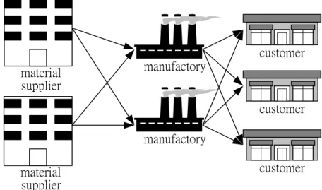
This study, based on the characteristics of bicycle industry, used the following assumptions (see Figure 1): 1. Concrete material flow processes of bicycle are
simplified as: input of raw material – inventory of raw material --- product – inventory of product --- distribution; and this study focuses only on the model structure of production – inventory of product – distribution;
2. For bicycle manufacturers, this study considers the problems of production and distribution for multiple periods and multiple products as demands vary because of factors such as the international economy, weather, etc;
3. Since demand for th is product will vary due to factors such as weather, the season, or holidays; a one year time period within the research period is marked as the planning period, and this planning period is divided into four separate parts, conforming to the annual seasons.
4. The industrial strategy of the industry has already employed BTO once an order is received; therefore, it is assumed that product demand is already known; 5. Only a single transportation system ‘land-sea’ is
considered.
material
supplier
material
supplier
manufactory
manufactory
customer
customer
customer
Figure 1 Research Domain
3.2 Designation of Parameters and Variables kt
p : Selling price of product k at period t;
jkt
d : Estimated demand of product k at period t in the locality j;
ijkt
α : Unit delivering cost of product k at period t from manufactory i to the point of demand j;
ikt
β : Unit production cost of product k at period t in manufactory i during ordinary working hours;
ikt
γ : Unit production cost of product k at period t in manufactory i during overtime working hours;
ikt
δ : Unit inventory cost of product k at period t in manufactory i;
jkt
δ : Unit shortage cost of product k during period t at the locality of demand j;
ikt
a : The consumption amount of the needed material r for producing per product k at period t in manufactory i;
irt
f : The upper bound value of the useable material r at period t in manufactory i;
ikt
b : The production time needed for producing per product k at period t in manufactory i;
it
η : The upper bound value of ordinary working hours at period t in manufactory i;
it
c : The upper bound value of overtime working hours at period t in manufactory i;
ikt
h : The minimal safety inventory for product k at period t in manufactory i;
it
θ : The upper bound value of safety inventory at period t in manufactory i;
ikt
x : The production amount of product k at period t in manufactory i during ordinary working hours;
ikt
ω : The production amount during overtime working hours for product k at period t in manufactory i; ijkt
y : The amount of product k delivered at period t in manufactory i to the locality of demand j;
ikt
e : The inventory of product k at period t in manufactory i;
jkt
s : The shortage amount of product k during period t at the locality of demand j.
3.3 Model objective
(1) Maximize total profit
To pursue the maximum profit is one of the business objectives and equation (7) helps maximizing the total profits. Profit itself includes items such as revenue and cost, while cost embraces production cost (including both ordinary and overtime working hours), transportation cost, inventory cost, and shortage cost.
Max total profit = (revenue – production cost during ordinary working hours – production cost during overtime working hours – transportation cost for product – inventory cost of product – shortage cost of product)
0
1 1 1 1 1 1
1 1 1 1
Max T K kt m n ijkt m ikt ikt m ikt ikt
t k i j i i
m n m n
ijkt ijkt ikt ikt jkt jkt
i j i j z p y x y e s β γ ω α ε δ = = = = = = = = = = = − + + + +
∑∑ ∑∑
∑
∑
∑∑
∑
∑
(7)
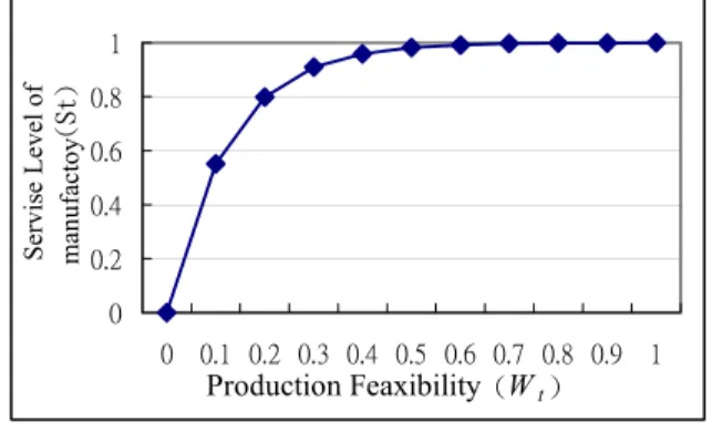
(2) Maximize the level of service in each period Under the assumed state that both the production time and transportation time of per unit product are fixed, a portion of the production time is used as the flexible time-space for adjusting to demand changes in order to satisfy the customers’ service needs. With this flexible period of time (spare production time in every period/total amount of time available for production in every period) as the crucial factor affecting the level of service, the assumption of relationship between the two can be indicated by the following formula.
Level of service l = f(spare production time in every period/total amount of time available for production in every period) 1 1 1 ( ), = 1, 2,..., 1 ( ) /( ) t t m K K
t ikt ikt ikt ikt it it
i k k Max S f W t T s.t. W b x b ω η c = = = = = −
∑ ∑
+∑
+ (8)If the manufacturer is confronted with defects such as
instability of demand and supply or mismanagement, it could provide delayed product delivery. And if the value of Wt is high, that indicates that there are many facilities
idle inside the factory to meet the urgent needs of customers: although a quality product could be generated there would be a low turnover. As a result, a trade-off relationship is created between the two objective equations, (13) and (14), in this study.
0 0.2 0.4 0.6 0.8 1 0 0.1 0.2 0.3 0.4 0.5 0.6 0.7 0.8 0.9 1 Production Feaxibility (Wt) S ervise Le ve l of manufactoy (St)
Figure 2 Relationship between Service Level of Manufacturer and Production Feasibility in t period
3.4 Model constraints
(1) Raw material Constraint
Raw material needed for production < amount of raw material provided
1
( )
1,..., ; 1,..., ; 1,...,
K
ikrt ikt ikt irt k a x f i m r R t T ω = + ≤ = = =
∑
(9) (2) Productivity ConstraintSince a manufacturer is constrained by plant and equipment, it is limited to a certain maximum production capability. And this study uses the bases production time as its unit.
Normal working hours X time needed for production with per unit normal working hours < maximal productivity during normal working hours
Overtime working hours X time needed for production with per unit overtime working hours < maximal productivity during overtime working hours
1 ; 1,..., ; 1,..., K ikt ikt it k b x η i m t T = ≤ = =
∑
(10) 1 ; 1,..., ; 1,..., K ikt ikt it k b ω c i m t T = ≤ = =∑
(11) (3) Inventory constraintDue to the constraint of space for inventory, it is essential that the total amount of product inventory in every period must be smaller than the limit of maximal inventory capacity. Furthermore, the product inventory this period should be equal to the total amount of inventory for the last period and amount for this period, subtracted by the amount distributed.
Amount of inventory product < maximal capacity of inventory
Amount of inventory this period = inventory capacity of the last period + production amount this period – amount of product distributed.
1 ; 1,..., ; 1,..., K ikt it k e θ i m t T = ≤ = =
∑
(12) ( 1) 1 ( ) 1,..., ; 1,..., ; 1,..., n ikt ik t ikt ikt ijktj e e x y i m k K t T ω − = = + + − = = =
∑
(13)(4) Relationship between the amount of product distribution and demand
The actual amount of product distributed has to be smaller or equivalent to the demands, as predicted in each locality, while the difference between the amount of distribution and demand will be the amount of shortage.
Amount of product distributed<=Estimated amount of demand
Shortage product = Amount of Product needed – Amount of Product distributed
1 ; 1,..., ; 1,..., ; 1,..., n ijkt jkt j y d j n k K t T = ≤ = = =
∑
(14) ; 1,..., ; 1,..., ; 1,..., m jkt jkt ijkt i s =d −∑
y j= n k= K t= T(15) (5) Non-negative constraint 0; 1,..., ; 1,..., ; 1,..., ikt x ≥ i= m k= K t= T (16) 0; 1,..., ; 1,..., ; 1,..., ikt i m k K t T ω ≥ = = = (17) 0; 1,..., ; 1,..., ; 1,..., ijkt y ≥ j= n k= K t= T (18) 0; 1,..., ; 1,..., ; 1,..., ikt e ≥ i= m k= K t= T (19)4. Illustrative Example: Bicycle
Manufacturer
In this section the real case of a bicycle manufacturer in Taiwan is examined to demonstrate that this model can be effectively well planed for providing good idea and thinking to treat supply-chain problems. The latest data for the management scenarios were obtained and that manufacturer data was put into this model, whereas each of the information is obtained as modified from the actual data. Section 4.1 provides the problem description and designation for the model; Section 4.2 shows the results and analysis of the operation; and Section 4.3 is sensitivity analysis and discussion.
4.1 Problem description and definitions
The operation problem of this practical example is designed to have three points of supply and seven points of demand, and the period of production programming is divided into four periods in each year. As learned from the case interviews, the demand for bicycle products varies seasonally, furthermore, bicycle has employed season as its different departments as different view-points from other high-tech products having high time cost and depreciation cost. As a result, in this study the first to the
fourth seasons are, respectively, July to September, October to December, January to March of the next year, and April to June. Since this study concerns only bicycles without power, the seven types of products used for product programming are mountain bikes, aluminum alloy bikes, light-weight bikes, children’s bikes, sport bikes, racing bikes, and carbon fiber bikes. The working hours of the manufacturing plant are designated as the six ordinary working days per week with twenty-four hours per day. Based upon the already known productivity of the three points of supply, it takes an average of thirty to forty hours to assemble a bicycle, and productivity constraint is rendered during the ordinary working hours in every season. The overtime working hours of the plant is the working hours in holidays.
4.2 Results and analysis
The operation in this part includes: (1) multi-objective compromise programming solution (MOCP), (2) weighted multi-objective programming solution (WMOP), (3) fuzzy multi-objective programming solution (FMOP), (4) weighted fuzzy multi-objective programming solution (WFMOP), (5) two-phase fuzzy multi-objective programming solution (TPFMOP). The results obtained are indicated in Tables 2 and 3.
Table 2 Multi-objective Programming Solution
Model
Outcome MOCP WMOP* FMOP WFMOP* TPFMOP Total profit (N.T.$*1000) 31038 7 456411 31133 6 493296 310925 1st period 0.93 0.92 0.93 0.89 0.93 2st period 0.95 0.93 0.95 0.89 0.95 3st period 0.79 0.68 0.79 0.58 0.79 4st period 0.88 0.87 0.88 0.76 0.88 *weights:4:1:1:1:1
As can be seen from Table 2, the value of the total profit by the weighted multi-objective model is far larger than the profit from the multi-objective compromise model, and it is the same for the service level for all periods. The magnitude of value change of the service level in the fourth period as programmed in the fifth model is rather limited, indicating there is more stable service quality, it is thus understood that the multi-objective weight obtained depends largely on the importance with which decision maker endows objectives. Furthermore, the size of the weighted value will have to be adjusted according the nature of the particular problem.
Comparing the results of fuzzy multi-objective, weighted fuzzy multi-objective, and two-phase fuzzy multi-objective programming, the maximum of the total profit value is from weighted multi-objective programming; and comparing this to a single objective, the maximization of the profit will be about the same. The objective value of the service level in each of the programming periods in the weighted fuzzy multi-objective model are similar to the programmed results of the profit maximization of a single objective. It
can thus be said that the model has almost lost its multiple objective significance. Since the programmed results of fuzzy multi-objective and two-phase fuzzy multi-objective are rather close, only the achieved value of total achievement in the two-phase multi-objective programming is larger by 0.001. If individual objectives
are analyzed, the objective of the two-phase fuzzy multi-objective programming – its resultant value – would be somewhat smaller than that of fuzzy multi-objective programming, while the achievement of the service level in each period is enhanced by 0.001, with an insignificant level of improvement.
Table 3 Cost Analyses of the Multi-objective Programming Model
Model MOCP WMOCP* FMOP WFMOP* TPFMOP
Outcome** Cost-Profit % Cost-Profit % Cost-Profit % Cost-Profit % Cost-Profit %
Total profit 2571618 - 2662507 - 2570337 - 2720545 - 2570034 - Total cost 2261231 - 2237054 - 2259001 - 2227248 - 2259109 - Material cost 1568831 0.69 1655888 0.74 1610677 0.71 1684356 0.76 1610528 0.71 Production cost (ordinary) Manufacturing cost 221504 0.10 227610 0.10 231246 0.10 229880 0.10 231149 0.10 Material cost 42474 0.02 0 0 0 0.00 0 0.00 0 0.00 Production cost
(overtime) Manufacturing cost 12565 0.01 0 0 0 0.00 0 0.00 0 0.00 Tax cost 212911 0.09 234169 0.10 212999 0.09 245300 0.11 213110 0.09
Transportation
cost Ocean shipping
cost 53630 0.02 61130 0.03 53535 0.02 67288 0.03 53471 0.02
Inventory cost 388 0.00 220 0 336 0.00 424 0.00 339 0.00 Stoket cost 148927 0.07 58038 0.03 150208 0.07 0 0.00 150511 0.07
*weights: 4:1:1:1:1; **Unit: hundreds N.
Comparing the results of the above-mentioned models in Table 3, it can be seen that material cost is the highest item of manufacturing cost for bicycles in terms of the total production cost, amounting to almost 70%; next is, the manufacturing cost, which amounts to 11% of the production cost. Thus, the production cost of this industry comprises 81% of the total cost, which shows that this industry is labor-intensive with high material cost. Despite the fact that the bicycle production has already been internationalized, and that its manufacturing, distribution, and selling behaviors are also multi-national, however, analysis of its costs indicates that it is not a high-tech product with high timing cost. Therefore, it is usually distributed by sea freight since that is inexpensive and the ratio of its cost to the total cost is almost negligible. However, the cost of custom can reach 10% of the total cost, amounting to the third highest cost item. As a result, the most important factor for the product sales of bicycle is the in-plant manufacturing cost and material cost of bicycle production, followed by export costs from the country of the manufacturing plant and the import taxes at the locality of demand. Of these three cost items, material cost is beyond the control of the bicycle manufacturer, so manufacturing cost and import and export taxes affect where the manufacturing plant is located.
After having compared multi-objective compromise model to two-phase fuzzy multi-objective programming, the difference of objectives between multi-objective compromise model and weighted multi-objective model programming are rather large, although, the objective
value of profit in multi-objective compromise is low. Even though the service level in each period of the weighted multi-objective model is not as high as that of the multi-objective compromise model, the programmed results of service level from 1st to 4th period of the
weighted multi-objective model, with the exception of 3rd
period (the service level of the 3rd period is about 0.7), are
all well over 0.8. In addition, the programmed results of fuzzy multi-objective model and two-phase fuzzy multi-objective model are much the same. However, the outcome of the weighted fuzzy multi-objective programmed model differs insignificantly from the programmed resolution of a single objective. Consequently, if the decision makers, having analyzed the results of each model, wish to achieve the programmed results of multi-objective production and distribution with maximum profit and highest quality service, using the weighted multi-objective model would be more compatible with these results.
4.3 Sensitivity analysis
Based on the conclusions above, the weighted multi-objective programming model is used to conduct the sensitivity analysis for the following policy. This policy is designed in three separate parts: (1) changes of unit production cost (manufacturing cost is increased by 20%, 40%, 60%, 80%, 100%); (2) changes of unit inventory cost (inventory cost is increased by 20%, 40%, 60%); (3) changes of unit shortage cost (shortage cost is lowered by 20%, increased by 20%, 40%).
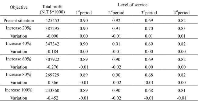
Table 4 Results of Changes to Unit Manufacturing Cost
Level of service Objective Total profit
(N.T.$*1000) 1stperiod 2stperiod 3stperiod 4stperiod
Present situation 425453 0.90 0.92 0.69 0.82 Increase 20% 387295 0.90 0.91 0.70 0.83 Variation -0.090 0.00 -0.01 0.01 0.01 Increase 40% 347342 0.90 0.91 0.69 0.82 Variation -0.184 0.00 -0.01 0.00 0.00 Increase 60% 307922 0.89 0.90 0.69 0.82 Variation -0.276 -0.01 -0.02 0.00 0.00 Increase 80% 269729 0.89 0.90 0.68 0.82 Variation -0.366 -0.01 -0.02 -0.01 0.00 Increase 100% 233360 0.89 0.90 0.68 0.81 Variation -0.452 -0.01 -0.02 -0.01 -0.01
Table 5 Results of Changes to Unit Inventory Cost
Level of service Objective Total profit
(N.T.$*1000) 1stperiod 2stperiod 3stperiod 4stperiod
Present situation 425453 0.90 0.92 0.69 0.82 Increase 20% 426902 0.90 0.91 0.70 0.83 Variation 0.003 0.00 -0.01 0.01 0.01 Increase 40% 426919 0.90 0.91 0.70 0.83 Variation 0.003 0.00 -0.01 0.01 0.01 Increase 60% 427384 0.90 0.91 0.70 0.83 Variation 0.005 0.00 -0.01 0.01 0.01
Table 6 Results of Changes to Unit Shortage Cost
Level of service Objective Total profit
(N.T.$*1000) 1stperiod 2stperiod 3stperiod 4stperiod
Present situation 425453 0.90 0.92 0.69 0.82 Increase 20% 430538 0.90 0.91 0.71 0.84 Variation 0.012 0.00 -0.01 0.02 0.02 Increase 40% 424601 0.89 0.91 0.69 0.82 Variation -0.002 -0.01 -0.01 0.00 0.00 Increase 60% 424562 0.89 0.90 0.69 0.82 Variation -0.002 -0.01 -0.02 0.00 0.00
(1) Changes of production cost: As can be seen from Table 4, the increase of production cost can impact the objective value of each objective in this study. With every increment of 20% to the manufacturing cost, the total profit would be lowered by approximately 9%. However, production cost has much less impact on the service level of each period.
(2) Changes of inventory cost: As indicated from Table 5, after inventory cost is increased by 20%, 40%, and 60% it will, on the contrary, increase both the total profits and the service levels in the 3rd and 4th periods.
(3) Changes of shortage cost: As seen in Table 6, the changes to shortage cost will have insignificant impacts on the five objectives studied in this research
because we have considered the feasible time-space for adjusting the demand change.
To sum up the analyses above, it is found that if the unit production cost increases, total profit will be reduced. In contrast, an increase of unit inventory cost will cause total profit to rise, although unit shortage cost has no impact on total profit. On the other hand, the increase of these three unit cost items will lead to the decrease of shortage cost and the increase of partial inventory cost, indicating that shortage cost will be reduced as of cost, so that inventory will be increased to meet the demand. This result shows that the inventory cost and shortage cost seem to have interactive behavior on the enterprise, whereas the enhancement of inventory cost will reduce shortage cost.
5 Conclusions and recommendations
5.1 Conclusions
Currently, most of the Taiwan bicycle manufacturers are OEM plants, so enhancement of service level has been one of their goals. In addition, both manufacturing and service industries are gradually induced to be customer service-oriented since stable customer service helps enterprise survival. As a result, this study uses the notion that production elasticity as partial spared productivity is more favorable than full production. This allows for demand space for adjustment to customer elasticity, and it increases the quality of customer service. Although such practice would lower enterprise profit because there is a trade-off relationship between these two objectives, this study uses multi-objective programming to meat this system.
This study uses five kinds of multi-objective programming methods for resolutions: multi-objective compromise programming, fuzzy multi-objective programming, weighted multi-objective programming, weighted multi-objective fuzzy programming, and two-phase fuzzy multi-objective programming. Comparing these five kinds of programming, it is found that the result from weighted multi-objective programming could be well received by the decision maker. The results of this are as follows:
Production cost is the highest of all the total cost items for bicycle production, amounting to 81%, which indicates that bicycle production is a labor-intensive and high material cost manufacturing industry. Besides, although bicycle manufacturing has multi-national production, distribution, and sales; its cost of time is relatively unimportant compared to that of high-tech industries. Thus its distribution is done by sea freight, whose cost is almost insignificant in terms of the total cost. However, expert and import taxes are the third highest cost item. Therefore, the greatest factor that affects the production and distribution of this industry would be the material cost of the product and manufacturing cost of the plant, followed by the export tax of the country where the manufacturing plant is located and the import tax at the locality of demand.
It is found that the total profit will be lowered when
unit production cost, unit inventory cost, unit shortage cost are increased. However, an increase of inventory cost will increase the total profit, while shortage costs have an insignificant impact on the total profit. If all three of these unit cost items are increased, that will lead to a decrease in the shortage cost and increase in the partial inventory cost, indicating that shortage quantity will be lowered because of cost, so inventory quantity should be increased to meet demand. Results of the kind show that inventory cost and shortage cost seem have interactive behavior on enterprises, in which the increase of inventory cost will lower shortage cost.
5.2 Recommendations
Recommendations offered in this study for subsequent research:
(1) Although this study has considered the service level of the manufacturer, assumptions were used for the function relationship between service level and production elasticity factor. Nevertheless, there are too many factors that affect the service level of manufacturer, so subsequent studies could focus on them for further investigation.
(2) In the planning model of this study, it is necessary to appreciate the weight relationship among each of the objectives; thus the preferences of the decision maker are extremely important.
(3) For practical management, the transaction price and manufacturing cost are not linear; transaction behavior allows discount and differential pricing, whereas manufacturing cost requires a factor as economic scale, in order to make the model realistic. In this study, there is further investigation on the problem of import and export, whose factors of influence are rather widespread and which is also one of the important issues in enterprise management. (4) The fuzzy multi-objective programming employed in
this study is simply a fuzzy objective equation, and fuzzy constraint equations can be added in subsequent studies.
(5) This model has only considered the issues of production and distribution, while upper-stream part supply is considered to be already known. Thus, relevant variables of changes from the upper-stream manufacturing supplier are been considered; if these could be considered, the model would be even more comprehensive.
Appendix
(I)
According to the explanation in Yu (1985),
d
∞should be used when the decision maker is focused on a certain objective. However,
d
1 is recommended when abalance of the objectives is required. The distance scale
P
d
found in the above-mentioned equation can also be standardized as follows:( )
( )
( )
( )
( )
( )
* 1 * 1 * * max ; 1, 2,..., max ; 1, 2,..., k i i p i i i i i p i i f f d i k f f f d i k f = = =∞ − = = − = = ∑
x x x x x x M(II)
Considering the shortest distance to the positive ideal solution (PIS) and the farthest distance from the negative ideal solution (NIS),
d
p can be indicated as follows:( )
( )
( )
( )
1 * * 1 p p k i i p i i i f f d f f− = − = − ∑
x x x x where,f
i( )
x
x∈X{
f
i( )
x
i}
−= min
, while
x
i is the solution relative tof
i*( )
x
. Generally speaking,f
i−( )
x
is anegative ideal solution.
(III)
(a) Determination of the ceiling and bottom limit of each of the objectives and constraint equations.
If it is assumed that the decision maker has the most satisfactory and ideal ceiling limit value
f
i(x
)
and thebottom limit value
f
i*(x
)
toward the ithobjective
f
i−(x
)
, then the decision maker can decide thevalues of the ceiling and bottom limit according to individual preference. Or the decision maker can take such objective as the function of the feasible solution space and find out the values through calculation, which is as shown in the payoff table.
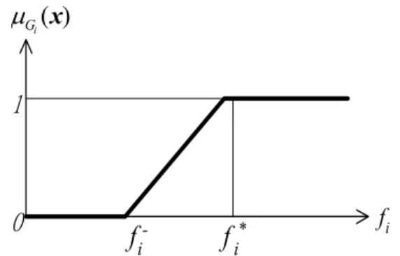
(b) Establishment of membership function
The membership function toward the ith fuzzy objective is as follows: * * * 0 ( ) ( ) ( ) ( ) ( ) ( ) ( ) ( ) ( ) ( ) 1 ( ) ( ) i i i i i G i i i i i i i f f f f f f f f f f f µ − − − − ≤ − = ≤ ≤ − ≥ x x x x x x x x x x x x as shown in Figure A.
f
i-f
i*1
0
f
i)
(x
i Gµ
Figure A Membership Function of the Objective
(c) Set up the membership function for the decision making set
µ
D(
x
)
{
}
* , ( x ) min i( ), 1,..., D i j G i k µ = µ x =From the max-min operation equation, the feasible fuzzy set can be found at the intersection of the objective and constraint equation. Since the decision maker needs precise decision-making recommendations, the maximum value of the membership in this decision making set is required. As a result, the maximum is utilized, and the corresponding membership function is thus obtained.
{
}
{
}
* * ( ) max min ( ), 1,..., max min ( ), 1,..., i i D G G i k i k µ µ µ = = ≥ = x x x(d) Turn the multiple objectives into a single objective for resolution
Finally, this problem can be transformed into precise LP problem for resolution:
* max ( ) ( ) . . , 1,..., ( ) ( ) i i i i f f s t i k f f λ λ − − − ≥ = − ≤ ≥ 0 x x x x Ax b x
Thus, general linear programming can be used for resolution.
References
[1] Bellman, R.E. and Zadeh, L.A. (1970), “Decision making in a fuzzy environment”, Management Science 17B(3), 141-164.
[2] Chandra, P. and Fisher M.L. (1994), “Coordination of production and distribution planning”, European Journal of Operational Research 72 (3), 503-517. [3] Dhaenens-Flipo, C. (2000), “Spatial decomposition
for a multi-facility production and distribution problem”, International Journal of Production
Economics 64(1-3), 177-186.
[4] Hwung, C.L. and Yoon, K. (1981), Multiple attribute decision making: methods and applications: a state-of-the-art-survey, Springer-Verlag.
[5] Lee, E.S. and Li, R.J. (1993), “Fuzzy multiple objective programming and compromise programming with Pareto optimum”, Fuzzy Sets and Systems 53(2), 275-288.
[6] Martinson, F.K. (1993), “Fuzzy vs. minmax weighted multiobjective linear programming illustrative comparisons”, Decision Sciences 24(4), 809-824. [7] Nagata, M., Yamaguch, T. and Komo, Y. (1995), “An
Interactive method for multi-period multiobjective production-transportation programming problems with fuzzy coefficients”, Journal of Japan Society for Fuzzy Theory and Systems 7(1), 153-163.
[8] Petrovic, D., Roy, R. and Petrovic, R. (1998), “Modelling and simulation of a supply chain in an uncertain environment”, European Journal of Operational Research 109(2), 299-309.
[9] Petrovic, D., Roy, R. and Petrovic, R. (1999), “Supply chain modeling using fuzzy sets”, International Journal of Production Economics 59(3), 443-453. [10] Tanaka, H., Okuda, T. and Asai, K. (1974), “On fuzzy
mathematical programming”, Journal Of Cybernetics 3(1), 37-46.
[11] Tzeng, G.H., Teodorovic, D. and Hwang, M.J. (1996), “Fuzzy bi-criteria multi-Index transportation problem for coal allocation planning of Taipower”, European Journal of Operational Research 95(1), 62-72.
[12] Van Der Vorst, J. G. A. J., Beulens, A. J. M., De Wit, W. and Van Beek, P. (1998), “Supply chain management in food chains: improving performance by reducing uncertainty”, International Transactions in Operational Research 5(6), 487-499.
[13] Yu, P.L. (1973) “A class of solutions for group decision problems. Management Science”, 19(8), 936-946.
[14] Yu, P.L. (1985), Multiple-criteria decision making:
concepts, techniques, and extensions, Plenum, New York.
[15] Zeleny, M. (1982), Multiple Criteria Decision Making, McGrew-Hill, New York.
[16] Zimmermann, H.J. (1978), “Fuzzy programming and linear programming with several objective functions”, Fuzzy Sets and Systems 1(1), 45-55.