Multiple-frequency range imaging using the OSWIN VHF radar:
Phase calibration and first results
Jenn-Shyong Chen1 and Marius Zecha2
1Department of Computer and Communications Engineering, Chienkuo Technology University,
Taiwan
2Leibniz-Institut für Atmosphärenphysik, Kühlungsborn, Germany
Manuscript accepted by Radio Science (November 2008)
Accepted
Corresponding author: Jenn-Shyong Chen
Add: Department of Computer and Communications Engineering,
Chienkuo Technology University, No. 1, Jieshou N. Rd., Changhua City 500, Taiwan
E-mail: [email protected]
Tel : +886-4-7111111 ext 2303, 2304 Fax: +886-4-7111163
Mobile Phone: +886-9-28128935
Offprint requests should be sent to Jenn-Shyong Chen 1 2 3 4 5 6 7 8 9 10 11 12 13 14 15 16 17 18 19 20 21 22 23 24 25 26 27 28 29 30 31 32 33 34 35
Multiple-frequency Range imaging using the OSWIN VHF radar:
Phase calibration and first results
Jenn-Shyong Chen1 and Marius Zecha2
1Department of Computer and Communications Engineering, Chienkuo Technology University,
Taiwan
2Leibniz-Institut für Atmosphärenphysik, Kühlungsborn, Germany
Abstract
This paper demonstrates the multiple-frequency range imaging (RIM) which was implemented recently on the OSWIN VHF atmospheric radar (54.1°N, 11.8°E), Germany. A simple but practical phase calibration method is introduced. We validate the RIM technique and the proposed calibration method successfully by examining various radar experiments with different pulse lengths, mono and coded pulses, evenly and unevenly spaced frequencies, and receiver filter bandwidths. The proposed calibration method not only mitigates the phase imbalance between the echoes received at different transmitting frequencies, but also provides a likely value of standard deviation (z) of the Gaussian range-weighting function for correcting the
range-weighting effect. Moreover, it is found that z can be adaptive to signal-to-noise
ratio when it is employed in practice; this procedure improves the continuity of the imaged powers of RIM around the boundaries of range gates, and an empirical expression has been proposed for this. With the improved power distribution around gate boundaries, we can obtain more available estimates of layer altitudes and exhibit the pass of the layer through gate boundaries clearly. Two observations are shown to demonstrate the maturation of the RIM technique used with the radar—convective cells and double-layer structures. These atmospheric structures cannot be seen clearly in the original presentation of signal-to-noise ratio (or height-time intensity) of the radar echoes having 150-m or 300-m range resolution.
Keywords: VHF radar, range imaging, phase imbalance, range weighting function Index terms: 6924, 6994, 6952 36 37 38 39 40 41 42 43 44 45 46 47 48 49 50 51 52 53 54 55 56 57 58 59 60 61 62 63 64 65 66 67 68
1. Introduction
Transmitting multiple frequencies to observe the atmosphere may become a basic capability of the modern mesosphere-stratosphere-troposphere (MST) radars. This observational technique starts with the frequency domain interferometry (FDI) using two slightly different frequencies [Kudeki and Stitt, 1987; Franke, 1990], takes wing after some sophisticated signal-processing algorithms such as the Capon method [Capon, 1969; Palmer et al., 1998] and the maximum entropy [Hysell, 1996], etc., were introduced to deal with the echoes received at several carrier frequencies, and is now known as range imaging (RIM) [Palmer et al., 1999] or frequency
interferometric imaging (FII) [Luce et al., 2001] in MST radar community.
The sophisticated algorithms used with RIM/FII are inversion processes, which were initially introduced to multiple-receiver coherent radar imaging (CRI) to determine multiple echo centers (angle of arrival or direction of arrival) in the radar volume [Hysell, 1996; Palmer et al., 1998]. With similar processing, these algorithms enable us to recognize multiple irregularity layers in the radar volume and then give estimates of the altitudes and thicknesses of the layers. Consequently, the range resolution of echo distribution (or brightness distribution) is improved greatly. With the information of layer altitude, layer thickness, and echo distribution, plenty of atmospheric studies have been carried out; for example, Kelvin-Helmholtz instability (KHI) [Chilson et al., 2003; Luce et al., 2007a], high-resolution wind profiling [Yu
and Brown, 2004], fine-scale layer structures [Chilson et al., 2001; Palmer et al.,
2001; Luce et al., 2006, 2007b], and vertical velocity bias associated with KHI [Chen
et al., 2008].
Recently, the OSWIN VHF radar (54.1°N, 11.8°E; Germany) has established the RIM/FII technique for the observations of the atmosphere. To validate the capability of the RIM/FII technique used with this radar is thus one of the purposes of this study. We starts with the essential workphase calibration in the RIM processing. Precise phase calibration can improve the continuity of the imaged powers at the boundaries of range gates, making the locations of the irregularity layers in the radar volume more reliable.
In the literature, several approaches have been employed for the phase calibration in RIM/FII; for example, reading the peak location of the FDI phase distribution (FDI phase is defined as the phase of the cross-correlation function of two echoes received by a pair of frequencies [Kilburn et al., 1995; Brown and Fraser, 1996]), measuring the initial phases of the carrier frequencies from the signals that are leaked from the transmitted signals back to the receiver by an ultrasonic delay line [Palmer et al., 2001; Chilson et al., 2001], applying the relationship between echo power and FDI 69 70 71 72 73 74 75 76 77 78 79 80 81 82 83 84 85 86 87 88 89 90 91 92 93 94 95 96 97 98 99 100 101 102 103 104 105 106
phase [Chen, 2004], utilizing genetic algorithms [Fernandez et al., 2005]. Among them the use of FDI phase distribution is simpler. Nevertheless, the shape of FDI phase distribution is related to some radar parameters, and usually, it needs enough radar echoes to obtain a reliable distribution in statistics; the latter could be a problem at times. For example, the mesosphere summer echoes (MSE), occurring in summer season at mid-latitudes, are striking VHF/UHF radar echoes that are related to variations of temperature and water vapor in the mesosphere, and can be observed for studying the waves/dynamics of the atmosphere around the mesopause height.
However, MSEs are sometimes weak and limited in time and height intervals. In view of this, in this paper we propose a new method of phase calibration. In addition to the phase calibration, an improved correction of the range-weighting function effect on the imaged power can also be achieved.
A brief description of the OSWIN VHF radar and the RIM method is given in section 2. In section 3, we detail the process of phase calibration with the proposed method and demonstrate several RIM experiments to validate the calibration method. Two initial RIM observations are shown in section 4. Finally, conclusions are stated in section 5.
2. Instrument and range-imaging technique
The OSWIN VHF radar, primarily operated at a central frequency of 53.5 MHz, can now generate the carrier frequencies from 53.25 MHz to 53.75 MHz with the smallest frequency step of 1 kHz. The carrier frequencies are generated with the same oscillator and can be changed from pulse to pulse to meet the basic requirement of RIM, that is, the echoes with various carrier frequencies are received almost simultaneously. Radar pulse shape can be Gaussian or rectangular and complementary codes are usually employed to raise signal-to-noise ratio (SNR). For more descriptions of the radar configuration/characteristics, browse the website
www.iap-kborn.de or refer to Latteck et al. [1999].
Among the inversion algorithms used with RIM/FII, the Capon method [Capon, 1969] is robust and handy [Palmer et al., 1999; Luce et al., 2001]. Without considering Doppler frequency sorting of the echoes, the Capon equations can be simply expressed as e R e 1 1 ) ( P r H , (1a) 107 108 109 110 111 112 113 114 115 116 117 118 119 120 121 122 123 124 125 126 127 128 129 130 131 132 133 134 135 136 137 138 139 140 141 142
nn
n
n
n
n
R
R
R
R
R
R
R
R
R
...
.
. .
.
...
...
2
1
2
22
21
1
12
11
R
, (1b) e=[ ej2k1r, ej2k2r,…, ej2knr ]T , (1c)where P(r) is the imaged power at the range r after range-scanning processing. The superscripts H and -1 in (1a) and T in (1c) represent, respectively, the Hermitian, inverse, and transposition operators. kn is the wavenumber of the n-th carrier
frequency. Rmn is the non-normalized cross-correlation function of the signals
calculated at zero-time lag for a pair of frequencies. Rmn can be simply written as
Rmn= <Rm Rn*> = <Amexp[j(-2kmrm+m] Anexp[j(2knrn-n)]>
= <AmAn exp [j2(knrn-kmrm) + (m-n)]>, (1d)
where <> means ensemble average. rm and rn indicate the ranges of the scatterers, and
m and n are the phase terms associated with the system responses to different
transmitting frequencies. After performing the ensemble average, the phase angle of (1d) is named FDI phase here. The phase terms m and n are not necessarily the same,
causing inaccurate range distribution of P(r). Many factors can contribute to the phase imbalance m-nfor example, the initial phases at different carrier frequencies, the
time delay of the signal in the media and radar system, and so forth. The major factors of the phase imbalance may vary from system to system and are difficult to identify exactly; however, it is possible to correct the phase imbalance by compensating suitable phase angle in Rmn. To find such suitable phase angle is thus essential and a
variety of approaches have been attempted, as mentioned in the introduction. There are two noticeable facts here: first, m-n is the phase difference between the two
signals, so absolute measurements of m and n are not necessary in the calibration;
second, Rmn is not normalized, so P(r) can indicate the echo distribution in range.
In addition to compensating the phase imbalance, the range-weighting effect on P(r) should be removed. This can be done approximately by using the inverse of the range-weighting function W2(r) = exp(-r2/z2) [Franke, 1990; Luce et al., 2001], where z is the parameter needed to determine appropriately for various radar experiments. 143 144 145 146 147 148 149 150 151 152 153 154 155 156 157 158 159 160 161 162 163 164 165 166 167 168 169 170 171 172
After the above corrections, P(r) may possess several distinct brightness maxima, indicating multiple layers in the radar volume. The resolvable number of layers in the radar volume depends on many factors, e.g., the frequency spacing and the maximum frequency separation, the distances between the layers and the layer thickness, the affection of SNR on some inversion algorithms like the Capon method, and so forth. As a start, we use five frequencies between 53.25 MHz and 53.75 MHz in the present RIM experiments although transmitting more frequencies are possible. The maximum frequency separation is 0.5 MHz and we transmit the pulse length 2 s. The use of the above radar parameters is partly subject to the capabilities/limitations of the present radar system and for the reason of protecting the radar system.
There have been many theoretical studies and simulations on RIM/FII, readers can refer to Palmer and Yu [1999], Yu and Palmer [2000], Luce et al. [2001, 2006] for more demonstrations of capabilities and limitations of RIM/FII.
3. Phase calibration
We carried out several radar experiments for the troposphere and lower
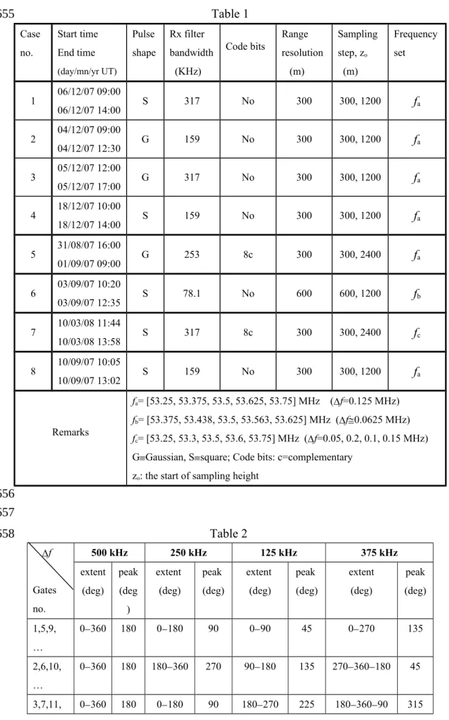
stratosphere with the RIM technique. Table 1 lists some important radar parameters employed for the experiments. Sampling time was ~0.2 s for these experiments, and 128 or 256 data points were used for one estimate of Rmn with (1d), resulting in the
time resolutions of about 30 s to one minute. It should be mentioned that some experiments were carried out with two or three observational modes alternately for multiple purposes; therefore the real time resolutions of the RIM results were double for the cases 6 and 8 (~2 min), and triple for the cases 14 (~3 min).
3.1 Distribution of FDI phases
As well known, the shape of FDI phase distribution at a range gate is closely related to the weighted radar volume formed by range weighting function and radar beam both. Range weighting function results from the receiver filtering process and can be approximated by a Gaussian form with the maximum at the center of the range gate [Doviak and Zrnic’, 1984]. On the other hand, the radar beam can be modeled by a two-dimensional Gaussian function on the plane perpendicular to the range direction and with the maximum at the beam centerline. There is a convolution of the beam shape function with the atmospheric echoes, causing the weighting of the echoes to be greatest at the center of the radar volume and decreases gradually outwards. As a result, the echoes returning from the irregularities closer to the center of the radar volume usually dominate the received power, causing the measured FDI phase to 173 174 175 176 177 178 179 180 181 182 183 184 185 186 187 188 189 190 191 192 193 194 195 196 197 198 199 200 201 202 203 204 205 206 207 208 209 210
deflect to the phase angle at the center of the radar volume. After collecting enough echoing situations, it is expected to obtain a quasi-Gaussian distribution of FDI phases with the peak at the phase angle predicted for the center of the radar volume, provided there is no phase imbalance between the echoes received at different carrier
frequencies. Such expectation is valid even for the echoes accompanied with noise (white noise). In theory, ensemble average in (1d) would eliminate the affection of noise on the FDI phase, and for pure noise the FDI phases are randomly, uniformly distributed, and should not be related to the range weighting function or radar beam shape.
The peak location of the FDI phase distribution at a range gate can be estimated in advance when suitable radar parameters are employed (e.g., frequency separation, pulse width, sampling time delay, sampling step, etc.). For example, with pulse width 2 s, sampling step 2 s, and sampling time delay 8 s (multiple of 2 s), Table 2 summarizes the extents of FDI phases of the grouped range gates as well as their peak locations at different frequency separations (f). As indicated, for f=500 kHz the FDI phases of all range gates inhabit between 0o and 360o, with a peak at 180o.
However, for f=250 kHz the FDI phases of odd and even range gates distribute over different phase extents and peak at different phase angles. As for f=125 kHz and 375 kHz, the FDI phases of the four grouped gates dwell in different phase extents and also peak at different phase angles. Such regularly distributed FDI phases make it possible to find the phase imbalance in (1d), as exhibited in Figure 1.
The panels (a)(d) of Figure 1 display the FDI phase distributions of four frequency pairs of the case 1 for different groups of gates. The results of other
frequency pairs unshown are similar to the displayed ones having the same frequency separation. To avoid unexpected affection of the noise, however, we used a SNR threshold, 0.125 (~-9dB), in adopting the FDI phase. Referring to Table 2, we can find that the peak locations of the distributions deflect to right slightly. For example, the frequency pair with f=250 kHz possesses two expected peak locations at 90o and
270o (see Table 2), but the observed distributions show two mean peaks at ~120o and
~300o. Apparently, there is a shift of ~30o in the observed distributions, that is, the
phase imbalance is ~30o. With similar inspection, the phase imbalances are ~60o,
~45o, and ~15o, respectively, for f=500 kHz, 375 kHz, and 125 kHz. Accordingly,
there is a linear relationship between the phase imbalance and the frequency separation.
The panel (e)(g) of Figure 1 shows the full FDI phase distributions of all
frequency pairs of the cases 1 (except for f=500 kHz). For saving pages, we display the integrated distributions of forty gates. For the situations of f=250 kHz and 125 kHz (panels (e) and (f), respectively), their respective humps in the distributions can 211 212 213 214 215 216 217 218 219 220 221 222 223 224 225 226 227 228 229 230 231 232 233 234 235 236 237 238 239 240 241 242 243 244 245 246 247 248
be identified definitely, and it is clear that the shift of the peak location depends only on the frequency separation, not on the absolute values of the two frequencies. As for the situation of f=375 kHz (panel (g)), it is difficult to distinguish the four peak locations shown in the panel (d). This is because the FDI phase distributions overlap largely and peak at different phase locations, causing the merged distribution
smearing. In conclusion, the phase imbalance depends only on the frequency
separation, which is similar to that examined by Chen [2004] for the Chung_Li VHF radar. This feature could be attributed to the group delay of the signals in the media and the time delay from the data processing in the radar system. To compensate these phase imbalances, therefore, we can simply consider a time delay (or range error) in the RIM analysis. The time delay is about (60o/360o)2s=0.333 s for the case here,
corresponding to a range error of ~50 m.
Figure 2(a)(c) shows the cases 24. For saving pages, only four of the
distributions are presented for each case. The unshown distributions are similar to the demonstrated ones having the same frequency separation. Generally speaking, it is more difficult to determine the phase imbalances here. This is partly because the pulse shapes and Rx filter bandwidths employed in the cases 24 result in shallower range weighting functions, causing the contrast between the peaks and the valleys in the FDI phase distributions smaller and less observable, especially for the observations with large frequency separations (e.g., f=500 kHz and 375 kHz). This points out one possible defect of using the FDI phase distribution for phase calibration when the experimental radar parameters produce a shallow range weighting function and/or the amount of the available echoes are not enough to reveal the range-weighting function shape. The following calibration method can avoid such inconvenience.
3.2 A new calibration method of FDI phase imbalance
Our new calibration method can find two desired parameters: the time delay for phase compensation and the standard deviation (z) of the Gaussian range weighting
function for range-weighting correction. The key thought/hypothesis is simple, that is, the imaged powers of RIM around the edge of two adjacent range gates should be very close after optimal range-weighting correction and phase compensation (by giving a corresponding time delay/range error in RIM). Based on this thought, the estimator given below can be employed to estimate the difference between the two sets of imaged powers, P1 and P2, around the edge of two adjacent range gates:
N 1 i 1i 2i 2i 1i N 1 i 1i 2i 2 2i 1i ) P P 2 -P P ( P P ) P -(P ERR , (2) 249 250 251 252 253 254 255 256 257 258 259 260 261 262 263 264 265 266 267 268 269 270 271 272 273 274 275 276 277 278 279 280 281 282 283 284 285where N is the number of the imaged powers. If P1=P2, then ERR=0. If P1P2, then
ERR>0 and ERR gets larger when the difference between P1and P2 is larger. Given
various values of time delay/range error and z to estimate P1 and P2, it is able to find
the smallest value of ERR. The time delay/range error and z with the smallest ERR
can be regarded as the optimal values in correcting the imaged powers. To compare with the phase imbalance obtained from the FDI phase distribution, however, the time delay/range error can be transformed into phase angle by regarding the change of FDI phase within a range-gate interval as 360o. Therefore, in practice we use the term—
(phase bias/360o)pulse length—for the time delay, in which the “phase bias” is the
variable given in the calculation. Such obtained optimal phase biases (and z) from
different pairs of range gates at different times would not be the same value due to some intrinsic uncertainties of the echoes, the inevitable noises, and the SNR-dependent result of the Capon method. However, a histogram of the optimal phase biases (and z) is able to indicate a likely value of phase bias (and z). We will see
this later.
Note that, with (2), we need the imaged powers outside of the nominal range gate; however, it is not necessary to use all of the imaged powers. For example, for the 2-s pulse length with 300-m range resolution, P1 can be the imaged powers
between 120 m and 180 m of the lower gate, and P2 can be the imaged powers
between -180 m and -120 m of the upper gate. If the scanning range of each gate is from -180 m to 180 m with 2-m scanning step, P1 contains the last thirty-one imaged
powers of the lower gate and P2 contains the first thirty-one imaged powers of the
upper gate. The scanning step can be smaller, say, 1 m, then P1 will be the last
sixty-one values of the lower gate and P2 contains the first sixty-one values of the upper
gate. Smaller scanning step consumes more calculating time but does not lead to observably different results according to our experience. Although one can employ the imaged powers within a larger range extent around the gate boundary, the range-weighting correction at the places far away the center of the range gate may be
excessive because the Gaussian range-weighting function is only an approximate form within the range gate interval. In view of this, we suggest using the imaged powers between -30 m and 30 m, centering on the height of gate boundary.
3.2.1. Mono pulses: cases 14
The cases 14 were examined again with the proposed calibration method, as shown in Figure 3. We summarize three important features as follows:
i) Left panels: The four histograms of the optimal phase biases exhibit similar shapes, and peak almost at the same phase angle ~70o, corresponding to a time
delay of ~0.389 s. This result is in good agreement with that obtained from the 286 287 288 289 290 291 292 293 294 295 296 297 298 299 300 301 302 303 304 305 306 307 308 309 310 311 312 313 314 315 316 317 318 319 320 321 322 323
FDI phase distributions of the case 1 (~0.333 s).
ii) Right panels: The distributions of z peak at about 150 m, 250 m, 190 m, and 190
m, respectively, which can be regarded as the likely values of z of their
respective Gaussian range-weighting functions. The difference in the likely values of z between the four cases arises from different pulse shapes and Rx filter
bandwidths employed (see Table 1). The experiment of the case 1 utilized square pulse with the Rx filter bandwidth of 317 KHz, producing a narrowest range weighting function compared with the other three experiments. On the other hand, the Gaussian pulse with the Rx filter bandwidth of 159 KHz in the case 2 results in a broadest range weighting function. Therefore, the likely values of z revealed
in Figure 3 make sense.
iii) The dispersion of phase biases and z in the histograms is related to low SNR. See
Figure 4 for further explanation.
In Figure 4, the left four panels show the two-dimensional histograms of the optimal phase biases and z, in which the number of each bin is indicated by gray
intensity. Darker pixel represents larger number and the gray intensity is
self-normalized. As indicated by the darkest pixels, the likely locations of phase biases of the four cases are almost the same (around 700), but the likely values of
z are
different. In the middle column, we can see that the optimal phase biases get more dispersive at lower SNR. This can be attributed to the noises which degrade the echoes and introduce statistical uncertainty into the estimated phase biases. The SNR here is the mean estimated from the sampled signals of two adjacent gates. In the right four panels, one can see the general relationship—a lower SNR correlates with a larger z. The fitting curves result from the equation
d -b a C ) SNR -(SNR 1 min z , (3)
where SNRmin is the threshold of SNR for fitting, and the value of -10 dB was used in
our studies. The constants a, b, c, and d are indicated in each panel. (3) is a more appropriate curve we have found so far for our experimental data. There may be various expressions for different radar experiments, and simpler formulas could also exist.
Figure 4 indicates that it would make the imaged powers at gate boundaries more continuous if we use the values of z and phase bias adaptive to SNR in correcting the
imaged powers of each gate. However, this is not practical. The optimal z and phase
324 325 326 327 328 329 330 331 332 333 334 335 336 337 338 339 340 341 342 343 344 345 346 347 348 349 350 351 352 353 354 355 356 357 358 359
bias are estimated from a pair of range gates, say, the first and the second range gates, and the second and the third range gates. Different pairs of range gates may result in different optimal z and phase bias. Consequently, there may be not consistent values
of z and phase bias for the second range gate. In practice, the imaged power and its
variations in range are small at low SNR, often making the phase calibration doubtful. Considering this, we can simply adopt the phase angle of the peak location revealed from the histogram of the optimal phase biases to correct all data. On the other hand, it would be good to use the z adaptive to SNR to improve the continuity of the
imaged powers around gate boundaries, especially in low-SNR condition. The fitting curve (3) can be employed to produce a suitable value of z at a given SNR.
Considering three consecutive range gates again, practical procedures are as follows: i) Estimate the mean SNRs of the first and the second gates, and the second and
third gates, respectively. Let the results be SNR1 and SNR2.
ii) Calculate the values of z from (3) with SNR1 and SNR2. Let the results be z1 and
z2.
iii) Use z1 for the first gate and the lower half part of the second gate, but use z2 for
the lower half part of the third gate and the upper half part of the second gate. With the above three steps, the upper and lower parts of the second/middle range gate usually suffer slightly different values of z, but this would smooth the imaged powers
at both boundaries of the second/middle gate. Repeating the above procedure, the continuity of the imaged powers at the boundaries of the third and the fourth gates, the fourth and the fifth gates, and so on, can be improved. It should be mentioned here that z is related to the radar parameters used, which does not depend on SNR in
theory. The feature of SNR-dependent optimal z is just due to the inevitable noises in
the echoes. Considering other factors may also vary the imaged power more or less, the above procedure of range-weighting correction is certainly not very perfect. Nevertheless, we will see that it indeed works in making the imaged powers more continuous at gate boundaries and is also beneficial for locating the imaged power centers or layer altitudes around gate boundaries (see below).
Figure 5 demonstrates one example of our studies. As seen, the SNR in the panel (a) shows some descending layer structures with severe smear in range. By contrast, range imaging exhibits the layer features much well (panels (b) and (c)). However, there is a difference between the two outputs of range imaging—the calibration processing results in more continuous imaged powers at gate boundaries (panel (c)) than that without any correction (panel (b)). A close-up of the brightness profiles at the time of 12:06 UT is shown in the panel (d). As seen, there are steep changes in the 360 361 362 363 364 365 366 367 368 369 370 371 372 373 374 375 376 377 378 379 380 381 382 383 384 385 386 387 388 389 390 391 392 393 394 395 396 397
uncorrected profile (black) at the heights of 6.9 km and 7.2 km (namely, at gate boundaries). After a range-weighting correction with z=150 m and phase
compensation, the profile (blue) peaks at gate boundaries, which is due to over-modification. To mitigate the steeply changed or over-modified imaged powers at gate boundaries, therefore, the range-weighting correction with SNR-dependent z
can be employed, as indicated by the red curve.
As mentioned, such smoothed powers at gate boundaries are beneficial for locating the layer altitudes. The locating results are shown in Figure 5(e)-(f), where the layer altitudes were estimated with the contour method proposed by Chen et al. [2008] for including the multiple-layer cases. In the panel (e), the layer altitudes estimated with 150-m z and adaptive z, respectively, are close; however, the use of
150-m z produces fewer available estimates of layer altitudes, causing many
discontinuities at gate boundaries, for example, the layer beginning at ~6.5 km and descending to ~4.5 km at ~12:00 UT. Such discontinuity of layer altitude is due to over-modification of the imaged powers. With a more appropriate value of z for this
case, e.g., 250 m according to Figure 2(b), we obtain the results shown in the panel (g). As seen, both layer altitudes are in good agreement. Based on this, 250 m has been an appropriate value of z for this case to correct the imaged powers as well as to
locate the layer altitudes. To be superior, adaptive z can be employed.
Note that although the value of z, 150 m, is not appropriate for the case here, it
is more suitable for the case 1. In any case, using adaptive z is suggested. To remind
readers here again, the use of adaptive z is to mitigate the steep change of the imaged
powers at gate boundaries; the value of z is theoretically not related to SNR, and its
likely value can be found with our new calibration method, namely, the peak location in the histogram of the optimal z (Figure 3).
3.2.2. Coded pulses: Case 5
Since coded pulses are usually utilized in radar observations to raise SNR, to validate the RIM experiment with coded pulses is essential for practical applications. One of the experimental results is shown in Figure 6, in which the coded pulses with 8-bit complementary codes were transmitted.
Figure 6(a) displays only some distributions of the FDI phases for saving pages; the unshown distributions are analogue to these distributions, depending on the frequency separation f. The features of these distributions are similar to the case 1, and according to Table 2, we can find the phase imbalance of each frequency separation easily. There is a linear dependence of phase imbalance on frequency separation except for the situation of f=375 kHz: ~80o, ~40o, and ~20o for f =500
kHz, 250 kHz, and 125 kHz, respectively, corresponding to a time delay of ~0.444 s. 398 399 400 401 402 403 404 405 406 407 408 409 410 411 412 413 414 415 416 417 418 419 420 421 422 423 424 425 426 427 428 429 430 431 432 433 434 435
Such time delay can also be found with the proposed calibration method, as indicated in Figure 6(b) and (c). As shown, the likely value of phase bias is ~90o, which is equal
to the time delay of ~0.5 s—very close to the value, 0.444 s, revealed from the FDI phase distributions. Other features of the optimal phase biases and z are also similar
to those of the cases 14. More experiments have been carried out with 2 and 4bit coded pulses, and their calibration results are alike (not shown). In view of these, the RIM technique with coded pulses is indeed workable for our radar system.
3.2.3. 4-s pulse length: case 6
A longer pulse length was employed in the case 6. Sampling range resolution was 600 m but the frequency separation was a half of that in the cases 15. Figure 7 shows the results. In the panel (a), the linear relationship between phase imbalance and frequency separation is not recognizable. By comparison, the panel (b) indicates clearly that the likely value of phase bias is around -60o and the values of the optimal
z gather at ~520 m. The likely phase bias is different from those of the cases 15.
The exact causes of such difference are unknown but could be associated with the radar parameters used. This reminds us that phase calibration is indeed necessary for the RIM experiments with different radar parameters. In addition, the optimal values of z are much larger here than those of the cases 15, which is due to the longer
pulse length (larger range resolution) employed. The dependence of optimal phase bias and z on SNR is also apparent, as shown in the panel (c), where we have used a
curve to fit the relationship between z and SNR.
3.2.4. Unevenly spaced frequencies: case 7
The case 7 is an experiment with unevenly spaced frequencies, which was carried out to validate the proposed calibration method further. Some of the integrated FDI phase distributions are displayed in Figure 8(a). Without any surprise, the
distributive aspects of f=500 kHz and 250 kHz are similar to the case 1. However, the uses of f=100 kHz and 50 kHz result in, respectively, five and ten peaks in the histograms. This makes sense because using f=100 kHz (50 kHz) causes different FDI phase extents within five (ten) consecutive range-gate intervals; each range-gate interval occupies 72o (36o). As for the situation of f=200 kHz, the FDI phases also
dwell in different extents within five consecutive range-gate intervals, but the phase span of each range-gate interval is 144o. Owing to considerable overlap of the FDI
phase distributions, it is difficult to distinguish the respective peaks in the integrated histogram of f=200 kHz; however, we can find the expected peaks by inspecting the respective histograms of all range gates, just as the situation of f=375 kHz shown in Figure 1. The above features also exist in the FDI phase distributions of other
436 437 438 439 440 441 442 443 444 445 446 447 448 449 450 451 452 453 454 455 456 457 458 459 460 461 462 463 464 465 466 467 468 469 470 471 472 473
frequency pairs of this experiment. Inspecting all FDI phase distributions, we can find again the linear relationship between the phase imbalance and the frequency
separation.
Figure 8(b) and (c) illustrate the calibration with the proposed method. As seen, the scenarios are the same as those of the cases 15. Figure 8(d) displays the SNR and the imaged power after calibration. As seen, the RIM method performs very well. A detailed examination of advantages and drawbacks of using unevenly spaced
frequencies in practical observation is an interesting issue but is not a main purpose of this study. We leave it aside for the moment.
4. More observations
Two observations are briefly shown here to demonstrate the excellent performance of the RIM technique used with the OSWIN radar.
Figure 9 displays a portion of the observations in the case 5. The original SNR is featureless (panel (a)), but the imaged powers (panel (b)) reveal some double-layer structures at the heights of ~4.5 km and ~5.5 km. Similar structure was also observed by Luce et al. [2006] with the MU radar in Japan. Double-layer structure is though to be related to KHI effect [Browning and Watkins, 1970; Worthington and Thomas, 1997] and so is in connection with vertical wind shear. Panel (c) illustrates the horizontal wind field derived from the full-correlation analysis (FCA) with the radar echoes, and the panel (d) shows the profiles of mean zonal and meridional velocities. As seen, the meridional component possesses more observable variations as well as larger vertical wind shear. If these double-layer structures are indeed in connection with the vertical wind shear observed, the meridional wind may be more crucial. Unfortunately, there are no temperature measurements nearby during the radar experiment and so it is difficult to examine this case further with the Richardson number or other parameters. It is thus suggested that radiosonde or lidar observation can be carried out along with the RIM experiment in the future.
Figure 10 shows an observation of convective condition (case 8). As seen, the original SNR reveals the convective structures roughly, but the imaged powers show three convective cells more clearly around the times of the beginning, 1100 UT, and the end of the observations, respectively. However, only the middle one was recorded completely. Also plotted are vertical velocities, indicated by short-vertical line
segments with black and red colors. It is interesting to see that stronger radar echoes appeared on the edges of the convective cells. This is not surprising because of the extremely different characteristics between the air parcels inside and outside the 474 475 476 477 478 479 480 481 482 483 484 485 486 487 488 489 490 491 492 493 494 495 496 497 498 499 500 501 502 503 504 505 506 507 508 509 510 511
convective cells, which causes severe variations in refractive index around the boundaries of the convective cells. Moreover, the vertical wind field combined with the imaged powers provides us a clearer observation of the atmospheric motion. For example, we can see large updrafts (~0.5 m/s maximum) in the middle of the
convective cell appearing around the time of 1100 UT, and observe downdrafts just on both sides of the updrafts. It should be mentioned that this case was carried out for other purposes with the receivers aligned in zonal, so the complete horizontal wind is not available.
5. Conclusions
There are two main purposes/contributions in this study: (1) validate the RIM technique implemented recently on the OSWIN VHF radar; (2) propose a simple but practical phase calibration method for the RIM processing, providing the following advantages/achievements:
1) Reveal the likely phase bias/time delay of the echoes without difficulty so far for various pulse lengths, pulse shapes, mono and coded pulses, and receiver filter bandwidths.
2) Can be applied to the RIM experiments with evenly and unevenly spaced frequencies.
3) Determine the value of z associated with the range weighting function. For
practical application, z can be adaptive to SNR in smoothing the imaged powers
at gate boundaries, which is beneficial for locating the layer altitudes around gate boundaries.
Two observations have been shown to demonstrate the excellent performance of the RIM method used with the radar, that is, double-layer structures, and convective cells with strong radar echoes on the edges of the cells and severe change of vertical velocities in the cells. Being the first attempt of using the RIM method on the OSWIN VHF radar and focusing on the calibration purpose, however, this study has not carried out a detailed investigation into the RIM data for scientific messages. Further studies/experiments are considering. Especially, it is expected in the near future that the RIM technique, combined with coherent radar imaging (CRI) and lidar
measurements, can be applied to the mid-latitude mesosphere summer echoes (MSE), detected overhead by the OSWIN VHF radar, and the polar mesosphere summer echoes (PMSE), observed in the polar region. Studies of wave activities,
microphysics, and dynamics of the MSE/PMSE can thus be improved with fine echo imaging (having the range resolution of several meters only) as well as from precise location of layer altitude.
512 513 514 515 516 517 518 519 520 521 522 523 524 525 526 527 528 529 530 531 532 533 534 535 536 537 538 539 540 541 542 543 544 545 546 547 548 549
Acknowledgements. This work was supported by the National Science Council of ROC (Taiwan) under Grant No. NSC95-2111-M-270-001-MY3. The OSWIN VHF radar is maintained by the Leibniz-Institut für Atmosphärenphysik (IAP) at
Kühlungsborn, Germany. The authors would like to thank the three anonymous referees for their valuable comments/suggestions on this study. 550 551 552 553 554 555
Table Captions
Table 1. Radar parameters used with the RIM experiments.
Table 2. FDI phase distribution and its peak location within the range of a gate. Pulse width: 2 s; sampling step: 2 s. Sampling time: 8 s.
Figure Captions
Figure 1. FDI phase distributions of the case 1 listed in Table 1. (a)(d): respective distributions of four frequency pairs for different groups of gates (see Table 2). (e)(g): integrated distributions of the first forty gates. Phase bin is 10o.
Figure 2. (a)(c): FDI phase distributions of the cases 24 listed in Table 1, integrated from the first forty gates. Phase bin is 10o.
Figure 3. Histograms of the optimal phase biases (left panels) and z (right panels).
(a)(d) show the cases 14 listed in Table 1. Phase bin is 10o, and
z bin is 10
m.
Figure 4. (a)(d) show the cases 14 listed in Table 1. Left column: 2-D histograms of the optimal phase biases and z with gray intensity. Central and right
columns: scatter plots of the optimal phase biases and z vs. SNR, respectively.
The fitting curves in the right four panels result from equation (3), with the constants of a, b, c, and d indicated in the panel (read from up to down in order). Figure 5. A partial observation of the case 2. (a) SNR. (b) Ranging imaging without phase and range-weighting corrections. (c) Range imaging with adaptable z
(varying with SNR) and phase compensation 80o. Scanning step is 2 m in the
imaging processing and time resolution is about three minutes. (d) A profiling comparison of the imaged powers of (b) and (c) at 12:06 UT, indicated by dark and red curves, respectively. The blue curve results from the use of z=150 m.
(e) and (f) are the comparisons of layer altitudes: (e) z=150 m (+) vs. adaptable
z (circle); (f) z=250 m (+) vs. adaptable z (circle).
Figure 6. For the case 5. (a) Same as Figure 2, (b) same as Figure 3, and (c) same as Figure 4.
Figure 7. For the case 6. (a) Same as Figure 2, (b) same as Figure 3, but z bin is 20
m. (c) same as Figure 4.
Figure 8. For the case 7. (a) Same as Figure 2, (b) same as Figure 3, and (c) same as Figure 4. (d) Left: SNR of radar echoes with the range resolution of 300 m. Right: range imaging with the scanning step of 2 m. Time resolution is about one minute.
Figure 9. For the case 5. (a) SNR of radar echoes with the range resolution of 300 m. (b) range imaging with the scanning step of 2 m. Time resolution is ~30 s. (c) horizontal wind field. (d) Profiles of mean zonal and meridional velocities, as 556 557 558 559 560 561 562 563 564 565 566 567 568 569 570 571 572 573 574 575 576 577 578 579 580 581 582 583 584 585 586 587 588 589 590 591 592 593
well as the horizontal wind speed.
Figure 10. For the case 8. Left: SNR of radar echoes with the range resolution of 300 m. Right: range imaging with the scanning step of 2 m. Red and black segments indicate, respectively, upward and downward velocities. A span of 300 m in vertical corresponds to 0.5 m/s. Time resolution is about two minutes.
594 595 596 597 598
References
Brown, W. O. J., and G. J. Fraser (1996), Frequency domain interferometry on spaced antenna MF radar, Radio Sci., 31, 1077–1088.
Browning, K. A., and C. D. Watkins (1970), Observations of clear air turbulence by high power radar,
Nature, 227, 260-263.
Capon, J. (1969), High-resolution frequency-wavenumber spectrum analysis, Proc. IEEE, 57, 1408-1419.
Chen, J.-S. (2004), On the phase bias of multiple-frequency radar returns of MST radar, Radio Sci., 39, RS5013, doi:10.1029/2003RS002885.
Chen, J.-S., G. Hassenpflug, and M. Yamamoto (2008), Tilted refractive-index layers possibly caused by Kelvin-Helmholtz instability and their effects on the mean vertical wind observed with multiple-receiver and multiple-frequency imaging techniques, Radio Sci., 43, RS4020,
doi:10.1029/2007RS003816.
Chilson, P. B., R. D. Palmer, A. Muschinski, D. A. Hooper, G. Schmidt, and H. Steinhagen (2001), SOMARE-99: A demonstrational field campaign for ultrahigh-resolution VHF atmospheric profiling using frequency diversity, Radio Sci., 36, 695–707.
Chilson, P. B., T.-Y. Yu, R. G. Strauch, A. Muschinski, and R. D. Palmer (2003), Implementation of range imaging on the Platteville 915-MHz troposphere profiler, J. Atmos. Oceanic Technol., 20, 987-996.
Doviak, R. J., and D. S. Zrnic’ (1984), Reflection and scattering formula for anisotropically turbulent air, Radio Sci., 19, 325-336.
Fernandez, J. R., R. D. Palmer, P. B. Chilson, I. Häggström, and M. T. Rietveld (2005), Range imaging observations of PMSE using the EISCAT VHF radar: Phase calibration and first results, Ann.
Geophys., 23, 207–220.
Franke, S. J. (1990), Pulse compression and frequency domain interferometry with a frequencyhopped MST radar, Radio Sci., 25, 565-574.
Kilburn, C., S. Fukao, and M. Yamamoto (1995), Extended period frequency domain interferometry observations at stratospheric and tropospheric heights, Radio Sci., 30, 1099–1109.
Kudeki, E., and G. R. Stitt (1987), Frequency domain interferometry: A high resolution radar technique for studies of atmospheric turbulence, Geophys. Res. Lett., 14, 198–201.
Latteck, R., W. Singer, and J. Höffner (1999), Mesosphere summer echoes as observed by VHF radar at Kühlungsborn (54oN), Geophys. Res. Lett., 26, 1533–1536.
Luce, H, M. Yamamoto, S. Fukao, D. Hélal, and M. Crochet (2001), A frequency radar interferometric imaging (FII) technique based on high-resolution methods, J. Atmos. Solar-Terr. Phys., 63, 221– 234.
Luce, H., G. Hassenpflug, M. Yamamoto, and S. Fukao (2006), High-resolution vertical imaging of the troposphere and lower stratosphere using the new MU radar system, Ann. Geophys., 24, 791–805.
599 600 601 602 603 604 605 606 607 608 609 610 611 612 613 614 615 616 617 618 619 620 621 622 623 624 625 626 627 628 629 630 631 632 633 634 635 636
Luce, H., G. Hassenpflug, M. Yamamoto, M. Crochet, and S. Fukao (2007a), Range-imaging observations of cumulus convection and Kelvin-Helmholtz instabilities with the MU radar, Radio
Sci., 42, RS1005, doi:10.1029/2005RS003439.
Luce, H., G. Hassenpflug, M. Yamamoto, and S. Fukao (2007b), Comparisons of refractive index gradient and stability profiles measured by balloons and the MU radar at a very high vertical resolution in the lower stratosphere, Ann. Geophys., 25, 47–57.
Palmer, R. D., T.-Y. Yu, and P. B. Chilson (1999), Range imaging using frequency diversity, Radio
Sci., 34, 1485–1496.
Palmer, R. D., P. B. Chilson, A. Muschinski, G. Schmidt, T.-Y. Yu, and H. Steinhagen (2001), SOMARE-99: Observations of tropospheric scattering layers using multiple-frequency range imaging, Radio Sci., 36, 681–693.
Worthington, R. M., and L. Thomas (1997), Long-period unstable gravity-waves and associated VHF radar echoes, Ann. Geophys., 15, 813-822.
Yu, T.-Y, R. D. Palmer, and D. L. Hysell (2000), A simulation study of coherent radar imaging, Radio
Sci., 35, 1129–1141.
Yu, T.-Y., and W. O. J. Brown (2004), High-resolution atmospheric profiling using combined spaced antenna and range imaging techniques, Radio Sci., 39, RS1011, doi:10.1029/2003RS002907.
637 638 639 640 641 642 643 644 645 646 647 648 649 650 651 652 653 654
Table 1 Case no. Start time End time (day/mn/yr UT) Pulse shape Rx filter bandwidth (KHz) Code bits Range resolution (m) Sampling step, zo (m) Frequency set 1 06/12/07 09:00 06/12/07 14:00 S 317 No 300 300, 1200 fa 2 04/12/07 09:00 04/12/07 12:30 G 159 No 300 300, 1200 fa 3 05/12/07 12:00 05/12/07 17:00 G 317 No 300 300, 1200 fa 4 18/12/07 10:00 18/12/07 14:00 S 159 No 300 300, 1200 fa 5 31/08/07 16:00 01/09/07 09:00 G 253 8c 300 300, 2400 fa 6 03/09/07 10:20 03/09/07 12:35 S 78.1 No 600 600, 1200 fb 7 10/03/08 11:44 10/03/08 13:58 S 317 8c 300 300, 2400 fc 8 10/09/07 10:05 10/09/07 13:02 S 159 No 300 300, 1200 fa Remarks fa= [53.25, 53.375, 53.5, 53.625, 53.75] MHz (f=0.125 MHz) fb= [53.375, 53.438, 53.5, 53.563, 53.625] MHz (f0.0625 MHz) fc= [53.25, 53.3, 53.5, 53.6, 53.75] MHz (f=0.05, 0.2, 0.1, 0.15 MHz)
GGaussian, Ssquare; Code bits: c=complementary zo: the start of sampling height
Table 2 f Gates no. 500 kHz 250 kHz 125 kHz 375 kHz extent (deg) peak (deg ) extent (deg) peak (deg) extent (deg) peak (deg) extent (deg) peak (deg) 1,5,9, … 0360 180 0180 90 090 45 0270 135 2,6,10, … 0360 180 180360 270 90180 135 270360180 45 3,7,11, 0360 180 0180 90 180270 225 18036090 315 655 656 657 658
… 4,8,12, … 0360 180 180360 270 270360 315 90360 225 659 660