以脈衝式電源驅動的軸對稱均勻氙氣電漿產生真空紫外光輻射之數值模擬研究

國

立 交 通 大 學

機

械 工 程 學 系

博

士 論 文

以脈衝式電源驅動的軸對稱均勻氙氣電

漿產生真空紫外光輻射之數值模擬研究

Numerical Investigation of VUV Emission

from a Homogeneous Coaxial Xenon

Excimer Discharge Driven by Distorted

Bipolar Square Voltages

研

究 生：周欣芸

指導教授：吳宗信

博士

以脈衝式電源驅動的軸對稱均勻氙氣電漿產生

真空紫外光輻射之數值模擬研究

Numerical Investigation of VUV Emission from a

Homogeneous Coaxial Xenon Excimer Discharge Driven

by Distorted Bipolar Square Voltages

研 究 生： 周欣芸 Student：Shin-Yun Jou

指導教授： 吳宗信 Advisor：Dr. Jong-Shinn Wu

國 立 交 通 大 學

機 械 工 程 學 系

博 士 論 文

A Dissertation

Submitted to Department of Mechanical Engineering College of Engineering National Chiao Tung University

in partial Fulfillment of the Requirements for the Degree of Doctor of Philosophy

in

Mechanical Engineering 2011

Hsinchu, Taiwan

以脈衝式電源的軸對稱均勻氙氣電漿產生真空紫外光輻射之數值模

擬研究

學生 : 周欣芸 指導教授 : 吳宗信 博士

國立交通大學機械工程學系博士班

中文摘要

近年來，準分子紫外光(Excimer UV; EUV)燈管放光技術在工業方面有著廣 泛的應用，例如臭氧的生成及半導體矽晶圓的表面清潔等。準分子的產生是透過 電漿內部複雜的化學反應機制例如解離、激發等碰撞過程，而真空紫外光的發生 則是在準分子由受激態掉回基態時所釋放出的能量所致。由於此類電漿反應機制 相當複雜，以致於燈管的設計通常靠試誤法，需付出高額的時間及成本。因此本 論文的主要目的是藉由流體模式模擬工具了解 EUV 燈管的氣體放電機制。如 此，在使用不同的參數時，我們可以先預測難以在實驗下量測到的電漿特性。 這樣不但可以縮短EUV 燈管的設計時程而且可能得到更好的燈管設計。 本論文使用一維軸對稱流體模式進行 kHz 等級電源驅動的氙氣準分子燈

管電漿模 擬 。此程式以有限差分法進行數值離散，考慮 local mean energy approximation (LMEA)及簡化氙氣化學反應機制。由於電子質量很輕，可立即反 應 電 場 變 化 ， 以 電 子 在 一 個 週 期 內 隨 時 間 的 變 化 量 可 分 為 三 個 主 要 階 段 : pre-breakdown(前放電區)、breakdown (放電區；172 nm 真空紫外光放光最強烈階 段) 及 post-breakdown (後放電區) 階段。結果顯示真空紫外光放射效率在使用 distorted bipolar 方形波形的表現比使用正弦波波形為佳。主要歸因於以下兩種主 要的機制: 第一、在distorted bipolar 方形波形下外加電壓迅速抬升，電子在沒 有彈性碰撞損失下可以吸收更多能量進行解離、激發等碰撞反應產生更高濃度的 激發態原子進而增加172 nm 紫外光所放出的量。第二、在正弦波形下，外加電 壓的緩慢下降促進離子透過歐姆加熱方式吸收外加電場能量，而離子所吸收的能

量並不會用於解離、激發等碰撞反應，對整個放電系統而言是一種能量的浪費。 為了瞭解控制準分子紫外光燈放電的真空紫外光輻射效率，我們在distorted bipolar 方形波形電源驅動下變化四種參數包括外加電壓頻率、背景氣體壓力、 燈管的寬度及介電層的數量。結果顯示強烈的172 nm 紫外光放射均在放電區前 期發生，這與電子吸收能量的階段相當吻合;另外離子的能量吸收主要發生在放 電區的後期。令人驚訝的是，當調高頻率時，燈管的效率只有些微的增加;而隨 著燈管電極間寬度的增加，燈管的效率也大幅的增加。此外，172 nm 紫外光的 放射效率在600 torr 下有最大值。而只放置一個介電層的燈管效率的表現比兩端 都放置介電層的燈管為佳。 最後，在本論文中也進行背景氣體的加熱影響的研究。加入氣體加熱影響的 模擬結果可合理解釋電漿產生的真空紫外光輻射與背景氣體壓力的關連而在超 過某各臨界壓力電漿無法被點燃的現象的實驗結果。這主要歸因於兩個主要機 制，第一、在高壓 (P = 510 torr) 下，由於氣體加熱引起背景氣體不均勻分佈導 致離子轉換反應(2Xe+Xe+→ Xe2+)更為活躍進而增進Xe₂+與電子的合併反應，最 終使得電子數量無法維持電漿生成;第二、隨背景氣壓增加，電子彈性碰撞的能 量損失亦隨著增加，造成整體電子能量(溫度)下降，進而使得電漿強度減弱，這 反應機制在高氣壓下對電漿造成的影響更為顯著。

Numerical Investigation of VUV Emission from a Homogeneous

Coaxial Xenon Excimer Discharge Driven by Distorted Bipolar

Square Voltages

Student : Shin-Yun Jou Advisor : Dr. Jong-Shinn Wu

Department of Mechanical Engineering

National Chiao Tung University

Abstract

Recently, the excimer UV (EUV) lamp has found a wide range of applications in industry, for example, in ozone generation and surface cleaning for Si wafer in semiconductor fabrication process. The generation of EUV results from the reaction mechanism like ionization or excitation and other collision processes in the plasma. The occurrence of VUV is due to the process that excimer falls from various excited states to a ground state. However, its design was mostly based on the trial-and-error method, which is time-consuming and cost ineffective. Thus, the goal of this thesis is to predict and understand the plasma physics and chemistry inside an homogeneous EUV discharge through fluid modeling technique.

In this thesis, a self-consistent radial one-dimensional fluid model, considering local mean energy approximation (LMEA), along with a set of simplified xenon plasma chemistry is employed to simulate the discharge physics and chemistry. The discharge is divided into three-period regions; these include: the pre-breakdown, the breakdown (most intense at 172 nm VUV emission) and the post-breakdown periods. The results show that the efficiency of VUV emission using the distorted bipolar square voltages is

much greater than that using sinusoidal voltages, which is attributed to two major mechanisms. The first is the much larger rate of change of the voltage in bipolar square voltages, in which only the electrons can efficiently absorb the power from the applied electric field in a very short period of time. Energetic electrons then generate a higher concentration of metastable (and also excited dimer) xenon that is distributed more uniformly across the gap, for a longer period of time during the breakdown process. The second is the comparably smaller amount of “wasted” power deposition by Xe₂+ _{in the post-breakdown period, as driven by distorted}

bipolar square voltages, because of the nearly vanishing gap voltage caused by the shielding effect resulting from accumulated charges on both dielectric surfaces.

Emitted powers of EUV light and deposited powers to the charged species of a homogeneous coaxial xenon discharge driven by the distorted bipolar square voltages are simulated by varying the test conditions of four key parameters, which include the driving frequency, gas pressure, gap distance and number of dielectric layers. Results show that there are three distinct periods that include pre-breakdown, breakdown and post-breakdown ones. It is found that intensive EUV (172 nm) emission occurs during the early part of the breakdown period, which correlates very well in time with the power deposition through electrons. In addition, power deposition through _{Xe and} +

2

Xe+ occurs mainly in the breakdown period and later part of breakdown period, respectively. Surprisingly, the emission efficiency of 172 nm increases only slightly with increasing driving frequency of power source, while it increases dramatically with increasing gap distance. In addition, the maximum emission efficiency is found

to take place at gas pressure of 600 torr. The emission efficiency of one-dielectric case is found to be better than that of two-dielectric one. The underlying mechanisms in the above observations are discussed in detail in the paper.

Finally, gas heating is included in the fluid modeling by a heat conduction equation for xenon. With this consideration, one can explain reasonably well the experimentally observed VUV emission at various background pressures, especially the extinguishment of the discharge as pressure exceeds some threshold value. The major mechanisms of the above phenomena are described as follows: 1) Increasing pressure leads to higher gas heating because of increasing electron energy loss through the elastic collision with xenon atoms in the bulk region; and 2) The above leads to higher gas density at outer region of the gap (r≈ 1.1~1.16 cm), because of heat conduction and assumed uniform pressure distribution, as compared to the case without gas heating which promotes the three-body Xe+-to-Xe2+ ion conversion and

e-Xe2+ recombination that greatly reduces the plasma density as pressure exceeds

Acknowledgements

首先，感謝我的論文指導教授吳宗信老師，無論是學業上的指導或是生活 上的言教與身教都讓我獲益良多。 也感謝本次口試指導委員陳彥升博士、徐振哲助理教授、魏大欽副教授及 劉耀先助理教授所提供的寶貴意見，因為你們的意見，使的本篇論文的內容更為 充實。 再來，感謝研究室的電漿模擬團隊夥伴們，捷粲、孟樺、沅明、凱文、必 任、昆模和穎志，沒有你們的幫助，就沒有這篇論文的產生，這也讓我體驗到團 隊合作無間的精神。 而本篇論文的產生，須感謝工研院材化所的學研合作計畫，謝謝魏碧玉博 士讓我們機會接觸到Excimer UV 燈管的領域。沒有這合作計畫，就沒有本篇論 文的產生。 更感謝我的家人與小國的一路相伴，尤其是父母親的支持，是我完成學業 地一大助力。爸、 媽，你女兒拿到學位了! 研究室的單車夥伴們，允民、 哲維、凱文與沅明，與你們一起騎單車穿梭 於新竹的鄉間山路及 17 公里海岸線那段時光真的很快樂，也為研究室的生活增 添幾許色彩，謝謝你們給的美好回憶，也希望日後還有機會一起騎車。 這段旅程雖然漫長，但終究還是抵達終點，面對下一段旅程，我會以謙卑 及踏實的心態，從容的面對。

Table of Contents

中文摘要

... I

Abstract ... III

Acknowledgements ...VI

Table of Contents ... VII

List of Tables ... X

List of Figures ...XI

Nomenclature ... XV

Chapter 1

Introduction... 1

1.1 Background and Motivation ...1

1.1.1 History and Applications...1

1.1.2 Dielectric Barrier Discharges...2

1.1.3 Breakdown Mechanism...3

1.1.4 Overview of Excimers...4

1.2 Discharge Control ...5

1.3 Literature Survey...6

1.3.1 Xenon Excimer Discharges Driven by the Sinusoidal Voltages.6 1.3.3 Gas Heating in Gas Discharges...7

1.4 Objectives and Organization of the Thesis...8

1.4.1 Specific Objectives...8

1.4.2 Organization of the Thesis...9

Chapter 2

Fluid Modeling... 11

2.1 Basic Equations of Fluid Modeling ...11

2.1.1 Continuity Equations...11

2.1.2 Electron Energy Density Equation...13

2.1.3 Field Equation...14

2.1.4 General Boundary Conditions...15

2.1.5 VUV Emission Efficiency...16

2.1.6 Discharge Current, Dielectric Voltage and Gap Voltage...17

2.2 Numerical Method and Algorithms... 17

2.2.2 Parallel Fully Implicit Newton-Krylov-Swartz-Algorithm...18

Chapter 3

Validation of the Fluid Modeling in Xenon Discharge

Simulation... 19

3.1 Xenon Plasma Chemistry ... 19

3.2 Case-1: 1-D Homogenous Planar Xenon discharge... 20

3.2.1 Simulation Conditions...20

3.2.2 Results and Discussion...20

3.3 Case-2: 1-D Homogenous Cylindrical Xenon discharge ... 21

3.3.1 Simulation Condition...21

3.3.2 Results and Discussion...21

3.4 Brief Summary of This Chapter... 22

Chapter 4

Enhancement of VUV Emission from a Homogeneous

Coaxial Xenon Excimer Ultraviolet Lamp Driven by

Distorted Bipolar Square Voltages ... 24

4.1 Discharge Properties by Sinusoidal Voltages ... 24

4.1.1 Phase Diagrams of Key Discharge Properties...24

4.1.2 Temporal Variation of Discharge Properties...28

4.2 Discharge Properties by Bipolar Distorted Square Voltages 30

4.2.2 Phase Diagrams of Key Discharge Properties...31

4.2.3 Snapshots of Key Discharge Properties...35

4.2.1 Temporal Variation of Discharge Properties...39

4.3 General VUV Emission Power and Efficiency ... 41

4.3.1 Characteristics of Power Deposition and VUV Emission...41

4.3.2 Comparison of VUV Emission Efficiency between Sinusoidal and Distorted Bipolar Square Voltages...42

4.4 Brief Summary of This Chapter... 45

Chapter 5

Parametric Study of VUV Emission from a Homogeneous

Coaxial Xenon Excimer Ultraviolet Lamp Driven by

Distorted Bipolar Square Voltages ... 47

5.1 Typical Characteristics of Power Deposition and VUV

Emission ... 47

5.2 Simulation Conditions ... 52

5.3 Effect of Frequency Variation... 52

5.4 Effect of Background Gas Pressure Variation ... 54

5.5 Effect of Gap Distance Variation... 56

5.6 Effect of Varying the Number of Dielectric Layers ... 58

5.4 Brief Summary of This Chapter... 59

Chapter 6

Effect of Gas Heating on VUV Emission from a

Homogeneous Coaxial Xenon Excimer Ultraviolet Lamp

Driven by Distorted Bipolar Square Voltages ... 61

6.1 Heat Conduction Equation ... 61

6.3 Results and Discussion... 63

6.4 Brief Summary of This Chapter... 68

Chapter 7

Conclusion and Recommendations of Future Work... 70

7.1 Conclusion... 70

7.1.1 Enhancement of VUV Emission from a Coaxial Xenon Excimer Ultraviolet Lamp Driven by Distorted Bipolar Square Voltages ...70

7.1.2 A Parametric Study of VUV Emission from a Coaxial Xenon Excimer Ultraviolet Lamp Driven by Distorted Bipolar Square Voltages...71

7.1.3 Effect of Gas Heating on VUV Emission from a Coaxial Xenon Excimer Ultraviolet Lamp Driven by Distorted Bipolar Square Voltages...72

List of Tables

Table 3-1 Reaction channels of the xenon discharge ... 75 Table 4-1 Power transfer efficiency between sinusoidal and bipolar square voltages... 76 Table 5-1 Test conditions for the parametric study... 77

List of Figures

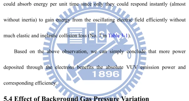
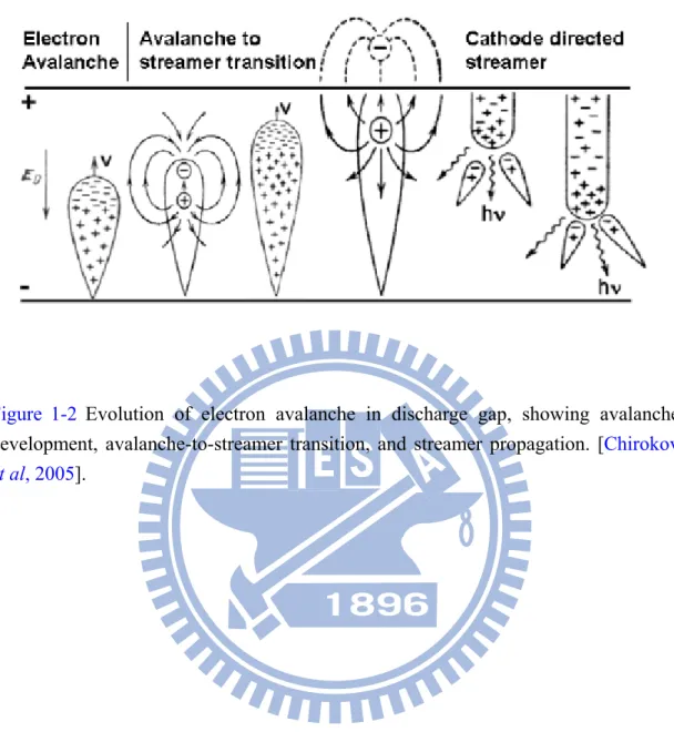
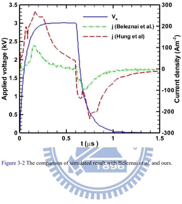
Figure 1-1 Common planar and cylindrical dielectric-barrier discharge configurations. [Kogelschatz et al, 1999]... 78 Figure 1-2 Evolution of electron avalanche in discharge gap, showing avalanche development, avalanche-to-streamer transition, and streamer propagation. [Chirokov et al, 2005]... 79 Figure 3-1 Reaction processes in a Xe discharge. ... 80 Figure 3-2 The comparison of simulated result with Beleznai et al. and ours. ... 81 Figure 3-3(a) A sketch of the coaxial xenon excimer lamp and (b) The configuration of the coaxial xenon excimer lamp. ... 82 Figure 3-4 The comparison with simulated result and experimental data. ... 83'

Figure 4-1 Spatiotemporal diagram of the number densities of charged species: electron (upper), atomic xenon ion (middle) and molecular xenon ion (bottom). ... 84 Figure 4-2 Spatiotemporal diagram of the number densities of excited

species: Xe*(met) (upper), * 3

2

Xe ( _Σu+) _{(middle) and electron temperature}

(bottom)... 85

Figure 4-3 The temporal variations of (a) applied voltage (Va), dielectric

voltage (Vd), gap voltage (Vg), discharge current density at inner side

(r=0.8 cm) and accumulated charge (Qa) and (b) the number density of

electron, the ion species Xe+ andXe₂+, the main excited species Xe*(met), the

main excimer species * 3

2

Xe ( Σ_u+) and Te utilizing sinusoidal waveform over a cycle. ... 86 Figure 4-4 Spatiotemporal diagram of the number densities of charged species: electron (upper), atomic xenon ion (middle) and molecular xenon ion (bottom). ... 87

Figure 4-5 Spatiotemporal diagram of the number densities of excited

species: Xe*(met) (upper), * 3

2 Xe ( u)

+

Σ (middle) and electron temperature

(bottom)... 88 Figure 4-6 Two snapshots of total species of (a) and (b) in the period I, (c) and (d) in the period II-1, (e) and (f) in the period II-2, (g) and (h) in the period III... 92

Figure 4-7 The temporal variations of (a) applied voltage (Va), dielectric

voltage (Vd) and gap voltage (Vg) in upper figure (b) discharge current

density at inner side (r=0.8 cm) and accumulated charge (Qa) in bottom

figure utilizing distorted square voltages over a cycle... 93 Figure 4-8 The temporal variations of number density of electron, the ion

species Xe+ andXe₂+_{, the main excited species Xe}*_{(met), the main excimer}

species * 3

2

Xe ( _Σu+) _{and Te during the period t=0 ~ 2 (μs). ... 94}

Figure 4-9 The power emission in the upper figure and power deposition utilizing distorted square voltages over a cycle. ... 95

Figure 4-10(a) The efficiency and P172 under different power source. (b)

The deposition power and power partition under different power source... 96

Figure 4-11 The comparison of light power emission (P172) between

sinusoidal voltages (the upper figure) and distorted square voltages (the bottom figure). ... 97 Figure 4-12 The comparison of power deposition between sinusoidal voltages (the upper figure) and distorted square voltages (the bottom figure). ... 98 Figure 4-13 A snapshot of distributions of electron energy consumption components using distorted square voltages. ... 99 Figure 5-1 Spatial distribution of cycle averaged discharge properties: a) VUV light emissions across the gap b) power depositions of charged species across the gap... 100

Figure 5-2 Spatiotemporal diagram of: a) 172 nm line UVU light emission and b) electron power deposition... 101 Figure 5-3 Spatiotemporal diagram of power depositions: a) atomic xenon ion and b) molecular xenon ion... 102 Figure 5-4 Effect of frequency on: a)η , P172 tot and P172, b) power deposition

of various charged species, and c) fraction of power deposition for different charged species at 400 torr of gas pressure, 4.5 mm of gap distance and 2 dielectric layers. ... 104

Figure 5-5 Effect of gas pressure on: a) η , P₁₇₂ tot and P172, b) power

deposition of various charged species, and c) fraction of power deposition for different charged species at 50 kHz of power source, 4.5 mm of gap distance and 2 dielectric layers. ... 106 Figure 5-6 Spatial distribution of cycle-averaged power densities of various charged species at different gas pressus: a) electron, b) atomic xenon ion and c) molecular xenon ion. ... 108

Figure 5-7 Effect of gap distance on: a) η , P₁₇₂ tot and P172, b) power

deposition of various charged species, and c) fraction of power deposition for different charged species at 50 kHz of power source, 400 torr of gas pressure and 2 dielectric layers...110 Figure 5-8 Spatial distribution of cycle-averaged power densities at different gap distances: a) VUC emission and b) ions and electron...111 Figure 5-9 Effect of number of dielectric materials on: a) η , P₁₇₂ tot and P172,

b) power deposition of various charged species, and c) fraction of power deposition for different charged species at 50 kHz of power source, 400 torr of gas pressure and 4.5 mm of gap distance...113 Figure 5-10 Spatial distribution of cycle averaged properties for one and two dielectric cases: a) electric field and b) power densities of charged species at 50 kHz of power source, 400 torr of gas pressure and 4.5 mm of gap distance. ...114

Figure 6-1 Comparison of the experimental and simulated data with and without gas heating. ...115

Figure 6-2 The spatial variations of background gas temperature (Tg) at

different pressures across the discharge gap. ...116 Figure 6-3 The spatial variation of ionic ohmic heating and electron energy loss due to elastic collision with xenon at different pressures with gas heating. ...117

Figure 6-4 The spatial variations of background gas temperature (Tg) w/ k

= const at different pressures across the discharge gap. ...118

Figure 6-5 The variation of thermal conductivity in the region of Tg = 400 –

700...119

Figure 6-6 The distribution of Tg at r =1 cm in the region of 100 – 513 torr.

... 120

Figure 6-7 The spatial distribution of background gas temperature (Tg)

and number density (Ng) at 510 torr across the discharge gap... 121

Figure 6-8 The comparison of temporal variations of charge species and Te

at 510 torr between with gas heating and without gas heating... 122

Figure 6-9 The comparison of spatial variations of Xe+-to-Xe2+ ion

conversion and e-Xe2+ recombination at 510 torr between with and without

gas heating. ... 123

Figure 6-10 The temporal variations of a) applied voltage (Va) and electron

number density (Ne) b) electron temperature (Te) in the range of

p=100-510 torr over a cycle. ... 124 Figure 6-11 Temporal distribution of electron power densities in period 0-2 (μs) at different gas pressures. ... 125 Figure 6-12 Temporal distributions of electron elastic collision loss power densities in period 0-2 (μs) at different gas pressures... 126

Nomenclature

ε The dielectric constant

f The power source frequency

P The gas pressure

Pin The input power density

Pout,k The light output power density generated from kth kind of

excited species

Te The electron temperature

iT The discharge curren

iC The conduction current

iD The displacement current

Va Applied voltage

Vd The dielectric voltage

Vg The gap voltage

S The source term

n The number density

μ The mobility

D The diffusivity

Γr The total flux

ψ The electric potential

Er The electric field

e

ε The electron energy

Chapter 1

Introduction

1.1 Background and Motivation

1.1.1 History and Applications

Because of its relatively low cost and low pollution, the excimer ultraviolet (EUV) lamp has found wide applications since its debut in a form of dielectric barrier in xenon gas in 1988 [Eliasson and Kogelschatz, 1988]. These include, for example, surface cleaning [Kane et al., 2004], plasma display [Park et al., 2007], LCD backlighting [Shiga et al., 2001], water quality purification [Safta, 2004], material deposition [Buck et al., 1998] and material processing [Zhang and Boyd, 1996] in the semiconductor industry. EUV lamp emission is caused by the excimer falling from excited states to the ground state. An excimer (originally short for excited dimer) is an unstable dimeric with a lifetime of about 10 ns. The important features of an excimer include: emission with narrow wavelength bandwidth, high efficiency and free radiation direction. Two typical examples are the formation of *

2

Xe or XeCl * excimer complexes. The EUV lamp has a dielectric barrier-type discharge which is a high-pressure non-equilibrium transient discharge. A primary function of the dielectric barrier is that it can suppress the occurrence of arc discharge, thereby preventing

damage to the metallic electrodes.

Because the plasma physics and chemistry inside the EUV lamp are very complex and difficult to measure, its design still heavily depends on the trial-and-error method that is both time-consuming and costly. Thus, detailed simulation of excimer discharge physics and chemistry could become a viable method for understanding the complicated plasma physics inside the lamp which, in turn, would lead to a better design.

1.1.2 Dielectric Barrier Discharges

The dielectric barrier discharge is a very high-pressure non-equilibrium transient discharge which usually consists of many tiny parallel current filaments showed in Figure 1.1 [Kogelschatz et al., 1999]. The barrier plays a role in producing high-energy electrons and suppressing arc discharges if micro-filament discharge has started. A primary feature of the lamp is that the dielectric barrier suppresses the occurrence of arc discharges and damage to the metallic electrode. Dielectric barrier discharge excimer lamps were originally driven by an alternating voltage, usually a sine wave. Under special conditions also homogenous discharges can be obtained. Most of the applications are operated up to now with filamentary discharges; but homogeneous discharges are coming up and open new perspectives.

[Chirokov et al., 2005]. If the electric field in the gas gap is sufficiently high to initiate avalanches, the breakdown starts with the Townsend phase. Next, a streamer occurs and a conducting channel-the filament-is formed. Charges are then transferred through the channel and accumulate at the dielectric surface. The voltage across the filament is finally suppressed and the discharge dies out. Group of local processes in the discharge gap initiated by avalanche and developed until electron current termination usually called microdischarge.

1.1.3 Breakdown Mechanism

The breakdown mechanism is based on the streamer theory, originally developed by Loeb [1960], Raether [1964] and Meek [1978]. A simplified conceptual development of a streamer begins with a single electron in an electric field. In the electric field the electron gains enough energy to ionize an atom or molecule, resulting in subsequent ionization and then an electron avalanche. This electron avalanche creates a strong positive field or streamer head within a small volume, which propagates across the gap, followed by a thin plasma channel (streamer). The streamer is a highly non-equilibrium plasma that is in a formative phase, with a small “head” that has a high space-charge limited field, and produces significant ionization through the presence of energetic electrons. The small head is followed by a “tail” with much lower electric field [Raizer, 1991]. Once the streamers bridge the gap

between the anode and the cathode, the plasma channel will become highly conductive and the discharge, an array of streamers, typically collapses to a single conducting channel.

1.1.4 Overview of Excimers

An excimer (originally short for excited dimer) is an unstable dimeric or heterodimeric molecule formed from two species, at least one of which is in an electronic excited state. The lifetime of an excimer is very short, on the order of nanoseconds. The feature of excimer include single wavelength, high efficiency and free radiation direction. The generation of excimer results from the reaction mechanism like ionization or excitation and collision process in the discharge. Emission of UV is due to the process that excimer falls from excited states to ground state. Excimer formation requires frequent three-body collisions and is therefore favored in a high-pressure discharge.

In general, excimer lamps utilize high-pressure rare-gas or rare-gas/halogen mixtures. Two typical examples are the formation of *

2

Xe or _{XeCl excimer} *

complexes. Firstly, the formation of * 2

Xe is formed essentially from neutral excited atoms (which Xe is the working gas). This process takes place in microdischarge channels and consists of three consecutive stages:

*

* * 2 Xe +2Xe→Xe +Xe (1.2) * 2 Xe →2Xe+hν (172 nm) (1.3) Secondly, the formation of XeCl* _{is formed mainly via recombination of ions with}

impurity in the working gas. A typical process consists of the following reaction steps: e−+Xe→e−+Xe++e − (1.4) 2 e−₊Cl _→Cl−₊Cl _(1.5) * Xe+₊Cl−_→XeCl _(1.6) * XeCl →Xe Cl UV radiation (308 nm)+ + (1.7) Other examples of excimer complexes may include, but not limit to, the rare-gas dimmers *

2

Ar radiating at 126nm, * 2

Kr at 146 nm, the halogen dimmers * 2 Cl at 259 nm, * 2 Br at 289 nm, * 2

I at 324 nm and the rare gas/halogen complexes _{ArCl at 175} *

nm, _{KrBr at 207 nm,} * _{KrCl at 222 nm,} * _{XeI at 253 nm,} * _{XeBr at 238 nm,} * *

XeCl at 308 nm [Gellert and Kogelschatz, 1991; Zang and Boyd, 1998].

1.2 Discharge Control

There exist a variety of methods to control dielectric barrier discharge. Besides voltage waveform, voltage amplitude, frequency, the electrode configuration, the number of the dielectric barriers and the kind of gas in the gap determine the microdischarge distribution and intensity. Thus, understanding the physical mechanism is very important in designing higher-efficiency excimer UV lamp.

1.3 Literature Survey

1.3.1 Xenon Excimer Discharges Driven by the Sinusoidal Voltages

Traditional excimer UV xenon lamps are driven by sinusoidal voltage waveforms, with discharge efficiency typically in the range of 10-20 %, and the discharge consists of multiple narrow filamentary channels [Stockwald and Neiger, 1995]. Simulation of xenon DBD driven by sinusoidal voltage waveforms using the one-dimensional planar fluid modeling has been proposed with gas pressures and frequencies in the range of 10-400 torr and 50 kHz – 1 MHz, respectively, by Oda et

al. [1999]. They found the efficiencies of spontaneous emission from excimers and

resonance-state atoms increase with an increase in the input powers for gas pressures higher than 50 torr. They have applied pulse voltages with trapezoidal and sinusoidal waveforms at different gap lengths. They have found in both waveforms the light output power depends not only on the amplitude of voltage waveforms but also on the discharge gap length. At the narrower discharge gap, the light output efficiency is improved by increasing the rate of increase of the applied voltage when the trapezoidal pulse is applied and by decreasing the duty ratio in the sinusoidal case. However, these waveforms were not realistic.

1.3.2 Xenon Excimer Discharges Driven by the Pulsed Voltages

experimentally (included transmission losses through the quartz and geometric loss) by using short (<750 ns) pulsed voltages interrupted by long idle periods (~ 40μs) [Vollkommer and Hitzschke, 1997]. Carman and Mildren [2003] found that VUV generation efficiency could reach 61% using very short voltage pulses through one-dimensional planar fluid modeling. Beleznai et al. [2006] compared the simulations results of a xenon EUV lamp (75 torr, driven by short voltage pulses) with the experimental data to validate their model using one-dimensional planar fluid modeling with very complex plasma chemistry in up to 99 reaction channels.Avtaeva and Kulumbaev [2008] have analyzed the difference of simulated results between two sets of different chemical reaction processes. However, there were no systematic simulations by varying all possible parameters for xenon excimer discharge driven by realistic pulsed voltages, which has been used in practical applications.

1.3.3 Gas Heating in Gas Discharges

Serikov and Nanbu [1997] have used 1-D particle-in-cell method to analyze gas heating effect in Argon gas. They analyzed the balance of power input into the gas due to the energetic neutrals, sputtered atoms and ions. Bogaerts et al [2000] extended the particle-in-cell method to 2D. It was found that the temperature can increase significantly at high voltages, pressures and currents. Revel et al [2000] have used a hybrid method to analyze gas heating effect in Argon gas. They found a large fraction

of the energy gained by the ions in the sheath. Benmoussa et al [2007] investigated the effect of gas heating near the electrode of an excimer lamp. However, the boundary conditions in predicting the gas temperature distribution are problematic. They have used temperature jump boundary conditions, which are not physical for a high-presure discharge. Belostotskiy et al [2008] measured experimental I-V characteristics of dc microdischarges in helium at different operating pressures (p = 300-800 torr) and found the classical scaling law of the cathode layer (sheath) did not apply if neglecting the influence of the neutral gas heating. Recently, we have observed experimentally [Lu, 2008] a peak VUV emissission illuminance at about 400 torr of background xenon and the discharge could not even sustain with a pressure larger than 440 torr. However, most simulation studies of the gas heating effect were focused on low-pressure discharges and lacking in high-pressure environment, although the type of operation condition is common in excimer lamp discharges.

1.4 Objectives and Organization of the Thesis

1.4.1 Specific Objectives

Based on previous reviews, the specific objectives of the thesis are summarized as follows:

homogeneous xenon excimer lamp driven by sinusoidal voltages via a self-consistent one-dimensional fluid modeling.

2. To understand the detailed discharge physics and chemistry in a co-axial homogeneous xenon excimer lamp driven by distorted bipolar square voltages and compare with those by sinusoidal voltages via a self-consistent one-dimensional fluid modeling.

3. To conduct a parametric study in a co-axial homogeneous xenon excimer lamp driven by distorted bipolar square voltage through a self-consistent one-dimensional fluid modeling and to understand the corresponding effects on the performance of the discharges.

4. To understand the gas heating effect on the performance of the co-axial homogeneous xenon excimer lamp driven by distorted bipolar square voltage through a self-consistent one-dimensional fluid modeling

1.4.2 Organization of the Thesis

According to the above objectives, this thesis is organized as follows:

Chapter 2 introduces the fluid modeling equations, numerical techniques we use to solve these equations for understanding the plasma physics and chemistry in the lamp.

simulation, in which two cases are used for this purpose.

Chapter 4 describes the comparison of the VUV emission efficiency of a coaxial xenon excimer ultraviolet lamp between sinusoidal voltages and distorted bipolar square voltages.

Chapter 5 describes the results of a parametric study of VUV emission from a coaxial xenon excimer ultraviolet lamp driven by distorted bipolar square voltages.

Chapter 6 describes the effect of gas heating on VUV emission from a coaxial xenon excimer ultraviolet lamp driven by distorted bipolar square voltages. Two important mechanisms which cause the extinguishment of the discharge is presented. The findings in this chapter are among the most important contributions in this thesis.

Chapter 7 summarizes the major findings of this thesis and the outline of the recommendations of future work.

Chapter 2

Fluid Modeling

2.1 Basic Equations of Fluid Modeling

In the framework of fluid modeling, electron and ion number densities are calculated as functions of time and space resulting from the coupled solution of the species continuity equation, species momentum equation, species energy equation, and field equations. Since the fluid modeling equations are similar for most of the gas discharges, we have only summarized a typical set of equations as the model equations for the purpose of demonstration. Note that we have not included flow convection effects in the present study.

2.1.1 Continuity Equations

The general continuity equation for ion species can be written as,

1 p i r p p p i n S t = ∂ + ∇ ⋅Γ = ∂

∑

r r p=1,…,K (2.1)

where n is the number density of ion species p, K the number of ion species, _p r _p

the number of reaction channels that involve the creation and destruction of ion species p, and Γr_p the particle flux that is expressed, based on the drift-diffusion approximation, as:

Γ =r_p sign q( )_p μ_{p p}n E D nr− _p∇r _p (2.2)

Er= −∇ϕ (2.3)

where _pq , Er , μ_p , D_p and α_iz are the: ion charge, electric field, electron mobility, electron diffusivity, and ionization rate, respectively. Note that the form of source term S_pi can be modified according to the modeled reactions describing how ion species p is generated or destroyed in reaction channel i. Boundary conditions at the walls have been applied, taking into consideration thermal diffusion, drift and diffusion fluxes.

The continuity equation for electron species e can be written as,

1 e i r e e e i n S t = ∂ + ∇ ⋅Γ = ∂

∑

r r (2.4)

where n_e is the number density of ions, r_e the number of reaction channels that invlve the creation and destruction of electrons, and Γr_e the corresponding particle flux that is expressed, based on the drift-diffusion approximation, as:

eΓ = −μe en E D n− ∇e e

r r

r

(2.5)

where _eμ andD_e are the electron mobility and electron diffusivity, respectively. These two transport coefficients can be readily obtained as a function of electron temperature from the solution of a publicly available computer code for the

be modified according to the modeled reactions which generate or destroy the ion in reaction channel i. Boundary conditions at the walls are applied, taking into consideration thermal diffusion, drift and the diffusion fluxes of electrons. Secondary electron emissions or photo-electron emissions from the solid walls can be readily added if necessary.

The continuity equation for neutral species can be written as,

1 uc i r uc uc uc i n S t = ∂ + ∇ ⋅ Γ = ∂

∑

r r uc=1,…,L (2.6)

where n_uc is the number density of uncharged species uc, L the number of neutral species, r_uc the number of reaction channels that involve the creation and destruction of uncharged species uc, and Γr_uc the corresponding particle flux, omitting convection effects, which can be expressed as:

ucΓ = −Duc∇nuc

r r

(2.7)

where D_uc is the diffusivity of neutral species. Similarly, the form of S_uci can also be modified according to the modeled reactions which generate or destroy the species in reaction channel i. Neumann boundary conditions at the walls are applied since surface reactions have not been considered in the present study.

2.1.2 Electron Energy Density Equation

(

)

1 3 c s e n e i i e B m e g i n m e E S n k v T T t ε M ε _ε = ∂ _{+ ∇ ⋅Γ = − Γ ⋅ − − −} ∂

∑

r r r (2.8) where 3 2 e B e n_ε ⎛_⎜= n k T ⎞_⎟

⎝ ⎠ is the electron energy density, T the electron temperature, e

i

ε the energy loss for the ith inelastic electron collision, k the Boltzmann constant, _B

m

ν the momentum exchange collision frequency between electron (mass m ) and _e

background neutral (mass M), T the background gas temperature, and _g Γr_nε the corresponding electron energy density flux, which can be written as:

(

)

5 5 2 2 e B e n B e e B e e m n k T k T k T m ε ν Γ =r Γ −r ∇ (2.9)

The second term on the right-hand side of Eq. (2.8) represents the sum of the energy losses of electrons due to inelastic collision with other species. The last term on the right-hand side of Eq. (2.8) can be ignored for low-pressure gas discharges, although it is important for medium-to-atmospheric pressure discharges. Similarly, boundary conditions at the walls have been applied, taking into consideration thermal diffusion, drift and diffusion fluxes. Secondary electron emission and other boundary effects may be readily added if needed.

2.1.3 Field Equation

Poisson’s equation for electrostatic potential distribution can be expressed as

1 ( ) ( K _{i i e}) i q n en ε ϕ = ∇ ⋅ ∇ = −

∑

− (2.10)

vacuum or dielectric permittivity, depending upon the problem.

2.1.4 General Boundary Conditions

Boundary conditions for the charge species fluxes towards the dielectric are defined as follows [Meunier, 1995; Boeuf, 1995; Veerasingam, 1997; Punset, 1998; Ivanov, 1999]: , 1 sgn( ) 4 i n a q μi in E n n vi th i Γ ⋅ =r r r⋅ +r (2.11) where nr is the normal vector pointing toward the dielectric and vth is the thermal

velocity , 8 B i th i i k T v m π

= in which T is temperature (K), kB is Boltzmann constant and

mi is the mass of charge species. The number a is set to be unity if the drift velocity is

directed toward the dielectric and to be zero otherwise: 1 sgn(q) E n > 0 0 sgn(q) E n 0 a μ μ ⎧ ⋅ = ⎨ ⋅ ≤ ⎩ r r

r r (sqn(q) presents species charge) (2.12) In the case of electrons, a flux towards to the dielectric is defined as follows:

,

1 4

e n aeμe en E n n ve th e

Γ ⋅ = −r r r⋅ +r (2.13) The boundary condition of continuity equation for neutral species uc is always set as the Neumann boundary, since no surface reactions are considered in this thesis. It is thus set as

0

uc n

Γ ⋅ =r r (2.14) The boundary condition of the electron energy density at dielectric surface is written

as

2 _{B e e}

n k T

ε

Γ ⋅ =r r Γr (2.15) The evolution of surface charge density on the dielectric barrier is calculated by integrating fluxes of charged particles directed to the barrier surface:

( _{i e}) e n t σ ∂ _{= Γ − Γ ⋅} ∂

∑

r r _r (2.16) It is assumed that charges remain on the barrier surface until recombining with charges of opposite sign.

2.1.5 VUV Emission Efficiency

Since we only considered one-dimensional radial fluid modeling, the input power density, Pin (or dissipated power), to the discharge is thus defined as:

2 1 2 2 ₀ 2 1 2 ( , ) ( , ) ( ) T r in _r c P j r t E r t rdrdt T r r = −

∫ ∫

(2.17) where T is the period of the applied voltage and jc is the conduction current density

caused by the electrons and ions. Note that r1 and r2 are the inner and outer radii of the gas gap. The VUV (vacuum UV) light output power density, Pout,k , generated

from the kth kind of excited species, is defined as:

2 1 , 2 2 ₀ 2 1 2 ( , ) ( ) T r k k out k _r k h n r t P rdrdt T r r ν τ = −

∫ ∫

(2.18) where hνk, τk and nk are the photon energy of the VUV light, lifetime and concentration of the excimer species, respectively. Thus, the VUV emission efficiency due to kth _{excimer species is given as:}

, out k k in P P η = (2.19)

2.1.6 Discharge Current, Dielectric Voltage and Gap Voltage

The discharge current iT(t) in this thesis defined as the sum of conduction current

iC(t) and displacement current iD(t) and is written as

iT(t) = iC(t) + iD(t) (2.20)

The voltage across the electrodes Vs(t) is written as

Vs(t) = Vd(t) + Vg(t) (2.21)

where Vd(t) is the total dielectric voltage across dielectric material(s) and Vg(t) is the

gap voltage across the gap that is filled with discharge gas.

2.2 Numerical Method and Algorithms

The numerical scheme and algorithms of the fluid modeling code, which was developed previously in our group and applied to simulate the EUV emission of xenon lamp, was introduced briefly in the following. Details of implementation can be found in Hung [2010].

2.2.1 Numerical Discretization

In this study, the above equations were recast into a one-dimensional form and discretized using the finite-difference method. The resulting system of nonlinear algebraic equations was then solved using a fully implicit backward Euler’s method in the temporal domain, with the Scharfetter-Gummel scheme for mass fluxes in the

spatial domain.

2.2.2 Parallel Fully Implicit Newton-Krylov-Swartz-Algorithm

At each time step, the resulting algebraic nonlinear system was solved by a parallel fully coupled Newton-Krylov-Swartz (NKS) algorithm [Caiet al 1998], in which the nonlinear discretized equations of a large sparse system was solved using an additive Schwarz preconditioned GMRES. The paralle code was implemented using physical domain decomposition method.

We have used an inexact or exact solution, such as incomplete LU (ILU) or LU factorizations, in each subdomain for the preconditioning. We evaluated the Jacobian matrix entries using a hybrid analytical-numerical method, in which the entries involving the derivative, with respect to number density (e.g. the source terms of species continuity equations), could be easily expressed analytically without resorting to numerical approximation. Other entries were evaluated using a standard finite-difference method. This strategy was especially useful for plasma simulations with a large number of species and reaction channels.

Chapter 3

Validation of the Fluid Modeling in Xenon

Discharge Simulation

In this chapter, we will present the validations of the one-dimensional fluid modeling by comparing with previous simulations and measurements. We first describe the xenon plasma chemistry we have used and then followed by the two cases of validations we have conducted. Finally, this chapter is concluded by summarizing the major findings.

3.1 Xenon Plasma Chemistry

In the current study, we have selected the xenon plasma chemistry that is basically the same as that used in Oda et al. [1999], which consists of 9 species and 24 reaction channels, as listed in Table 3-1 in order to save the computational time. These reaction channels included electron-neutral elastic collision (No. 1 in Table 3-1), direct electron impact ionization (No. 2 in Table 3-1), excitation (No. 3-5 in Table 3-1), stepwise ionization (No. 6 in Table 3-1), recombination (No. 7 in Table 3-1), heavy particle collision (No. 8-18 in Table 3-1) and radiation process among electrons, ions, associated excited atoms, excimer xenon and ground-state xenon atoms (No. 19-24 in Table 3-1). Figure 3-1 shows schematically these reaction channels using the

energy diagram for a better overview of the inter-relation among the species.

3.2 Case-1: 1-D Homogenous Planar Xenon discharge

3.2.1 Simulation Conditions

The test conditions are the same as in [Beleznai et al., 2006] and are briefly described as follows: pure xenon, a pressure of 75 torr, a frequency of 20kHz, a gap distance of 9.65 mm, dielectric thickness of 0.7 mm and applied voltage maximum of 3 kV. Simulation conditions we used are summarized as: 405 uniform grid points, a time step size in the range of 10-13 ~ 5×10-11 s, and parallel computation on four cores.

3.2.2 Results and Discussion

Figure 3-2 shows the comparison of the simulated discharge currents between the Beleznai et al.’s and ours in a cycle, Two large spikes are both found from the discharge currents in the two simulated results when the applied voltage fast rises and drops. The magnitude of the simulated spikes in our result are in reasonable agreement with that of Beleznai et al., although the simulation has not reproduced the multiple spikes. The reason could probably be attributed to that we have adopted a much simpler plasma chemistry than that of Beleznai et a. and also we have assumed a homogeneous discharge. Nevertheless, the trend of the discharge currents coincident with each other, which shows that the use of simple plasma chemistry can still capture most of the physics inside the xenon lamp.

3.3 Case-2: 1-D Homogenous Cylindrical Xenon discharge

3.3.1 Simulation Condition

Figure 3-3(a) depicts a sketch of the coaxial xenon excimer lamp simulated in the present study. For explaining the typical discharge physics and chemistry, we have selected the following simulation conditions for convenience (see Figure 3-3(b)). The tube length is 70 cm, the gap distance (d) in the radial direction is 3 mm, and both the inner and outer quartz tubes (di+do) are 1 mm thick. An inner-powered electrode with

a radius of 7 mm is placed in direct contact with the inner quartz tube and an outer mesh grounded electrode (~92% in porosity) with a radius of 12 mm is placed outside the outer quartz tube. The complicated three-dimensional geometrical structure is simplified as a one-dimensional radial coordinate system in the current study as the first step in understanding the discharge physics and chemistry without the complications of geometry. The dielectric constant of the quartz tube was 4.0, and power supply frequency f and xenon gas pressure p are fixed at 50 KHz and 400 torr, respectively.

3.3.2 Results and Discussion

Figure 3-4 shows the comparison of the simulated and the experimental discharge currents in a cycle. Note the experimental data were provided by Industrial Technology Research Institute in Taiwan. Several fast oscillating current spikes are

found from the measured currents, while only a single major spike is found from the simulated data. The reason should be we have employed one-dimensional radial fluid modeling to simulate the discharge physics. However, the magnitude of the simulated spike is reasonably comparable to that of the measured data. Note that the actual EUV lamp has a very complex three-dimensional geometric structure with a highly porous (~91%) outer grounded electrode. Also, the measured voltages are slightly more positive at the inner electrode than at the outer electrode in the post-breakdown period, which should be attributed to the auto-DC-bias effect because of the unequal area of the inner and outer electrodes. Note that the slightly negative current is within the experimental uncertainties of the current probe. In the current study, we do not take this into account in the simulation. However, based on the comparison between the 1-D radial fluid modeling and the experiments, we could conclude that the use of the one-dimensional radial fluid model is able to reasonably capture the major discharge physics inside the real EUV lamp.

3.4 Brief Summary of This Chapter

Major findings of this chapter are summarized briefly as follows:

1. For Case-1 validation, the trend of the two simulation discharge currents agree well with previous simulation data. However, the magnitude of the simulated spike in our result is not in quantitative agreement with that of Beleznai et al.’s,

which should be due to the simplified plasma chemistry.

2. For Case-2, the results of simulated and the experimental discharge currents agree reasonably well, although the complexity of electrode geometry is greatly simplified in the present simulation.

3 Based on the two validation cases, we can conclude that the present one-dimensional fluid modeling with the simplified plasma chemistry is capable of reproducing most of the plasma physics inside a typical xenon lamp operating at high pressures.

Chapter 4

Enhancement of VUV Emission from a

Homogeneous Coaxial Xenon Excimer

Ultraviolet Lamp Driven by Distorted Bipolar

Square Voltages

In this chapter, we present the enhancement of VUV emission from a coaxial xenon excimer ultraviolet lamp driven by distorted bipolar square voltages as compared to that driven by sinusoidal voltages. The simulation conditions are based on the Case-2 in Chapter 3. We first present the results of discharge properties by sinusoidal voltages in detail, which serves as the baseline for comparison. Then, the results of discharge properties by distorted bipolar square voltages are presented and compared to the sinusoidal case wherever is possible. Before concluding remarks, general VUV emission power and efficiency is presented. Finally, a brief summary is made at the end of this chapter.

4.1 Discharge Properties by Sinusoidal Voltages

4.1.1 Phase Diagrams of Key Discharge Properties

In this section, we present the simulation results of xenon discharge driven by sinusoidal voltage waveforms using phase diagrams of several important discharge

properties.

Figure 4-1 shows the phase diagrams of concentration of charged species (electron, atomic xenon ion and molecular xenon ion), while Figure 4-2 shows the phase diagrams of Xe*(met) and * 3

2

Xe ( _{Σ that are two important excited species for u}+) VUV emission (172 nm), and of the electron temperature. Note the red dashed and black solid curves in Figure 4-1 (top) represent the temporal variation of applied sinusoidal voltage and spatial-average number density of electrons in the gap. In general, the phase diagram can be divided into six periods according to the temporal variation of electron number density because the electrons can respond immediately to the variation of electric field. The periods I and IV are pre-breakdown regions, the periods II and V are breakdown regions and the periods III and VI are post-breakdown regions. In period II and V, it can be further divided into two sub-periods (II-1 and II-2; V-1 and V-2). The trend of species in the first half cycle (I, II and III) is similar to the second half cycle (IV, V and VI), except that the discharge current is opposite to each other and the species concentrations in the second half cycle is larger than those in the first half cycle because the electric field at inner side (r=0.8cm) is larger than at outer side (r=1.25cm) due to smaller radius of curvature. In the following, we only describe the discharge physics in the first half cycle for brevity.

Period I

In this pre-breakdown period, the total number of electrons decreases with time because the electrons are attracted to anode side and accumulated on the inner dielectric tube due to its rising voltage. Nearly no ionization occurs during this period as can be seen from the very concentration of the atomic xenon ions (middle of Figure 4-1) which originate from the direct electron impact ionization. Albeit the electron temperature is very high near the outer dielectric tube (cathode side) (bottom of Figure 4-2) due to the rising voltage at the inner electrode, the breakdown does not occur because of only very small number of electrons in that region. Similarly, both Xe*(met) and * 3

2

Xe ( _{Σ are very few across the gap in this period. However, near u}+) the inner dielectric tube (0.8-1.0 cm) the quasi-neutrality holds with the plasma density of ~5x1016 (m-3), while the molecular xenon ions (Xe₂+_{) prevails across the}

gap. At the end of Period I, the electric field near the outer dielectric tube (cathode side) increases to a value at which the breakdown occurs instantaneously at the start of Period II.

Period II

In Period II-1, the breakdown occurs at r≈1.1 cm and moves towards outer quartz tube in a speed of ~2,000 m/s (from anode towards cathode) (middle of Figure 4-1) by direct electron impact ionization, the number of electrons rapidly increases to the

maximal value within 1 μs at r≈1.18 cm and then decreases gradually afterwards (top of Figure 4-1). At the same time, number of molecular xenon ions increases rapidly in the same fashion through the three-body collision channel (No. 16 in Table 3-1), which also rapidly consumes the atomic xenon ions and the molecular xenon ions become the dominating ions in Period II-2 (bottom of Figure 4-1). In addition, both Xe*(met) and * 3

2

Xe ( _{Σ are very abundant because of the excitation of ground-state u}+) xenon by the energetic electrons (top and middle of Figure 4-1). Interestingly, the temporal location of where the maximal amount of * 3

2

Xe ( _{Σ occurs is shifted u}+) slightly after that of the maximal amount of Xe*_{(met) because the former is formed}

solely through the reaction between Xe*_{(met) and ground-state xenon (No. 12 in Table}

3-1). In Period II-2 that lasts less than 1 μs, the quasi-neutral region forms between the r≈1.1-1.2 cm and moves from cathode side (grounded) to anode side (powered) slowly, in which the Xe₂+ _{is the dominating ion species as described earlier. In}

addition, both Xe*(met) and * 3 2

Xe ( _{Σ disappear because of intense photon emission u}+) (172 nm) (No. 19 in Table 3-1) in this Period II-2. In the region of r≈1.0-1.2 cm, beginning from the later period of Period II-1, the electron temperature decreases rapidly with time because of the shielding by the increasingly accumulated charges on both quartz tubes and the electrons lose energy in ionizing the ground-state xenon. Period III

In this period, the quasi-neutral region expands slowly first from the cathode side (outer) towards the anode side (inner) with decreasing plasma density in the bulk (Figure 4-2). Later the electrons begin to move from the anode side (inner) towards the cathode side (outer) at t=5-6 μs, when the applied voltage decreases from the peak. In this period, both Xe*(met) and * 3

2

Xe ( _{Σ nearly do not exist because the electron u}+) temperatures are very low down to even 0.1 eV at the end of the Period III.

After Period III, the polarity of the applied voltage switches and the above described breakdown procedures repeat with opposite direction and location, however, with higher plasma density and more abundant excited species because of the stronger electric field near the inner electrode.

4.1.2 Temporal Variation of Discharge Properties

To further elucidate the discharge physics described in the above, we present temporal variation of several important discharge properties in Figure 4-3. Figure 4-3 shows the temporal variations of: a) the applied voltage (Va), the dielectric voltage

(Vd), the gap voltage (Vg), the discharge current density at inner side (r=0.8 cm) and

the accumulated charges (Qa) and b) the spatial-average number density of electron,

the ion species Xe+ and Xe₂+_{, the metastable species Xe}*_{(met), the excimer species}

* 3 2

Xe ( _{Σ and the electron temperature utilizing sinusoidal voltage waveform over a u}+) cycle. Note the dielectric voltage is defined as the sum of voltages across both quartz

tubes. Similarly, we divide the cycle into six periods as shown earlier in the description of Figure 4-3 for the purpose of easier discussion.

Period I

In Period I (pre-breakdown region), the dielectric voltage, the gap voltage and the electron temperature increase with increasing applied voltage, while both the magnitudes of accumulated charges at inner (less positive) and outer (less negative) quartz tubes, and the number densities of electron and Xe₂+ _{decrease with increasing}

applied voltage. The current density at inner quartz tube (r=0.8 cm) decreases slightly. The magnitudes of the accumulated charges at inner and outer quartz tubes decrease in this period because of incoming electrons and ions respectively as the applied voltage increases. In addition, all excited xenon species start increasing in this period because of rising electron energy,

Period II

Again, Period II (breakdown region) is divided into Periods II-1 and II-2. In Period II-1, the gap voltage has risen to some critical level that leads to very high electron energy, which makes the xenon breakdown. The abundant increase of charge species number density lead to a rapid increase of the current density at the inner dielectric surface, at which a large amount of electrons accumulate in a very short period of time.

In period II-2, Note the number density of Xe₂+ _{keeps increasing through}

three-body ion conversion channel (No. 18 in Table 3-1), so ion accumulated on the outer anode dielectric surface (see Figure 4-3). The combined accumulated effect on the inner anode and outer cathode dielectric surface results in a much smaller gap voltage (see Figure 4-3) by shielding out the applied voltage. The reduced electric field can not offer energy to electrons and keep discharge anymore. The number density of all species and electron temperature keep reducing.

Period III﹕

In period III (post-breakdown region), a turning point of applied voltage at t = 5×10-6 _{(s) can be found. According to the turning point, period III can be divided two}

sub regions III-1 and III-2. In sub period III-1, gap voltage and current density keep reducing, dielectric voltage keeps rising, Qa at inner side and outer side keep

accumulating. In sub period III-2, electron no longer accumulates on the inner dielectric again and turns back to the bulk. The direction of current density turns into opposite direction. Gap voltage becomes negative from positive. The main species in the region are electron and molecular ion, but they keep reducing due to wall loss and recombination effect.

4.2 Discharge Properties by Bipolar Distorted Square

Voltages

4.2.2 Phase Diagrams of Key Discharge Properties

Figure 4-4 shows the phase diagrams of the concentrations of the charged species (electron, atomic xenon ion and molecular xenon ion), while Figure 4-5 shows the phase diagrams of Xe*(met) and * 3

2

Xe ( _{Σ , two important excited species for u}+) VUV emission (172 nm) and electron temperature. Note that we have only shown

* 3 2

Xe ( _{Σ , instead of u}+) * 1 2

Xe ( _{Σ , because the concentration of the former was much u}+) greater than the latter. We divided these phase diagrams into six periods in the temporal directionaccording to the temporal variation of electron number density, as only electrons can respond immediately to variations in the electric field. Periods I and IV were pre-breakdown regions, Periods II and V were breakdown regions and Periods III and VI were post-breakdown regions. Periods II and V were further divided into two sub-periods (II-1 and II-2; V-1 and V-2). The trend of discharge in the first half cycles (I, II and III) was very similar to that of the second half cycles (IV, V and VI), except that the discharge currents were opposite to each other and there were some slight differences in the properties because of the different areas of the inner and outer electrodes. Note that the blue dashed curve in the top of Figure 4-4 represents the temporal variation of the spatial-averaged number density of electrons in the gap. For brevity, we have only described the discharge physics and chemistry in the first half cycles (I, II and III) in detail, as those in the second half cycles were

fundamentally the same, with the exception as mentioned earlier. Period I

In this pre-breakdown period, the spatial-averaged number of electrons decreased slightly with time because the electrons were attracted to the anode side (inner electrode) and accumulated on the inner dielectric tube due to its rising voltage. In the earlier part of Period I (negative applied voltage, 19.6-20 μs in both Figures 4-4 and 4-5), the concentrations of all species were low, especially the excited and meatastable xenon, because the electron energy was still quite low.

In the later part of Period I (positive applied voltage, 0-0.37 μs in both Figures 4-4 and 4-5), in the central region of the gap (r≈0.95-1.05 cm), the concentration of the atomic xenon ions (_{Xe ) increased up to ~10}+ 6_(cm-3_{), as a result of direct impact}

ionization, as shown in the middle of Figure 4-4. Although the electron temperatures were very high near the outer dielectric tube (cathode side) (see bottom of Figure 4-5) due to the rising voltage at the inner electrode, breakdown did not occur because of the very small number of electrons existing in that region (see top of Figure 4-4). At the same time, both the concentrations of Xe*(met) and * 3

2

Xe ( _{Σ increased to the u}+) order of ~1010 _(cm-3_{) in the central region of the gap. In addition, molecular xenon}

ions (Xe₂+_{) were abundant (>5×10}10 _cm-3_{) throughout the complete cycle; this result}

the inner dielectric tube (r≈0.83-0.94 cm), the quasi-neutrality was held with a plasma density of ~5x1010 cm-3 (

2

e _{Xe Xe}

n » n + ? n + ), while the molecular xenon ions (Xe2 +₎

prevailed across the gap. At the end of Period I, the electric field near the outer dielectric tube (r≈1.2 cm, cathode side) was gradually enhanced by the “cathode-directed streamer-like” ionization wave; this will be explained in a later section using snapshots of the discharge properties, at which point the breakdown occurred instantaneously at the start of Period II.

Period II

This breakdown period was further divided into two sub-periods, II-1 and II-2. In Period II-1, the breakdown occurred at r≈1 cm, where the number of electrons increased dramatically (see top of Figure 4-4), and moved towards the outer quartz tube at a speed of ~7,000 m/s (from anode towards cathode) by direct electron impact ionization. We termed this the “cathode-directed streamer-like” ionization wave; the details will be elucidated later. The number of electrons rapidly increased to the maximal value (>2x1012 cm-3) within ~0.3 μs at r≈1.22 cm, and then decreased gradually afterwards (see top of Figure 4-4). At the same time, the number of molecular xenon ions increased rapidly in the same fashion through the three-body collision channel (No. 18 in Table 3-1), which indeed rapidly consumed the atomic xenon ions’ , the molecular xenon ions thereby became the dominant ions in Period