低功率多工樹之輸入選擇編碼演算法

全文

(1)國立交通大學電子工程學系電子研究所碩士論文. 低功率多工樹之輸入選擇編碼演算法 Input Selection Encoding Algorithm for Low Power Multiplexer Tree. 研究生：張孝恩指導教授：黃俊達博士. 中華民國九十五年八月.

(2) 低功率多工樹之輸入選擇編碼演算法 Input Selection Encoding Algorithm for Low Power Multiplexer Tree Student: Hsiao-En Chang Advisor: Dr. Juinn-Dar Huang. 研究生：張孝恩指導教授：黃俊達博士. 國立交通大學電子工程學系. 電子研究所. 碩士論文. A Thesis Submitted to Department of Electronics Engineering & Institute of Electronics College of Electrical & Computer Engineering National Chiao Tung University in partial Fulfillment of the Requirements for the Degree of Master in Electronics Engineering & Institute of Electronics. August 2006 Hsinchu, Taiwan, Republic of China. 中華民國九十五年八月.

(3) 研究生：張孝恩. 指導教授：黃俊達博士國立交通大學. 電子工程學系電子研究所碩士班. 摘. 要. 隨著攜帶式設備的出現，功率消耗變成在VLSI設計上重要的考量之一。在VLSI 設計中，多工器是基本且常用的元件。ㄧ般而言，標準元件庫只提供2對1多工器和4對1多工器。不同大小的多工器在不同的設計裡都可使用到，因此通常多對1多工器會被拆解為用2對1多工器組成的樹狀實現。交換頻率(switching activity) 是影響功率消耗重要的因素之一。在此論文裡，我們針對在多工器樹裡面的每一個2對1多工器的交換頻率做最小化的處理。我們利用輸入訊號變成邏輯1的機率來分析在多工樹裡面每一個2對1多工器的交換頻率。我們解決的以下的問題: 給予輸入信號變成邏輯1的機率和輸入信號被選到的機率，我們提出的演算法有效率地給予每個輸入資料訊號輸入選擇編碼,同時依照每個輸入資料訊號輸入選擇編碼產生了最小化功率消耗的多工樹。最後，實驗結果顯示我們提出的演算法在64對1 多工器的情況下求出的功率消耗比平均功率消耗減少了24%。. i.

(4) Input Selection Encoding Algorithm for Low Power Multiplexer Tree Student: Hsiao-En Chang. Advisor: Dr. Juinn-Dar Huang. Department of Electronics Engineering & Institute of Electronics National Chiao Tung University. Abstract With the advent of portable devices, power consumption becomes one of most important considerations in the VLSI designs. Multiplexer (MUX) is a basic component that is commonly used in VLSI designs. In general, only 2-to-1 and 4-to-1 MUX are available in the standard cell library. Any size of MUX could be used in various design blocks. Usually, an n-to-1 MUX is decomposed as an equivalent tree of 2-to-1 MUXes. The switch activity is an important factor of power consumption. In this thesis, we focus on the minimization of the switch activity for each 2-to-1 MUXes in the MUX tree. We utilize the on probabilities of input signals to analyze the switching activity of 2-to-1 MUXes in a MUX tree. We solve the following problem: Given the on probabilities and the selection probabilities of input data signals, our proposed algorithm efficiently assigns each input selection encoding for input data signals. According to each input selection encoding of input data signals, a minimum power MUX tree is generated. Finally, the experimental results reveal that our proposed algorithm reduces up to 24% power dissipation for 64-to-1 MUX when compared to average power dissipation.. ii.

(5) 誌. 謝. 首先,我要感謝我的指導教授-黃俊達博士,在碩士兩年當中給我的支持和鼓勵,讓我能有良好的研究環境,在自由的學習風氣之下,培養出獨立研究的能力,又能隨時給予寶貴的意見及指導,對老師的感激之情,並非以簡短的文句可以表達。. 當然也要感謝養育我長大的父母對我的栽培,沒有他們,就沒有今日的我。接著要感謝的是所有來參與口試的所有教授們,黃婷婷教授,林永隆教授,和周景揚教授,百忙當中抽空前來指導我,讓我受益匪淺,也讓我得到了寶貴的經驗,謝謝你們。. 最後也要感謝所有實驗室的同仁們,阿光、維聖、士祐、翊展、詠翔學長、丁之暉、許哲霖、李南興學弟們,跟大家一起修課、做實驗、和討論及分析研究成果更是我人生旅途中一段最值得珍惜的回憶,希望未來在讀書或工作還有機會一起努力。. 希望這篇論文能對人類社會有小小的貢獻,如此一來在辛苦也就值得了,再次謝謝大家的幫忙。. iii.

(6) Contents Chinese Abstract.............................................................................................................…i English Abstract ............................................................................................................ ...ii Acknowledgments. ...................................................................................................... ....iii Contents ............................................................................................................................iv List of Tables ....................................................................................................................vi List of Figures................................................................................................................. vii Chapter 1 Introduction................................................................................................…1 1.1. Motivation ..................................................................................................…1. 1.2. Thesis Organization....................................................................................…2. Chapter 2 Preliminaries… ..........................................................................................…3 2.1. Power Dissipation of MUX… ....................................................................…3. 2.2. MUX Decomposition .................................................................................…5. Chapter 3 Previous Works..............................................................................................7 3.1. Problem Formulation of Bottom Up Heuristic Algorithm .............................7. 3.2. Bottom Up Heuristic Algorithm……………………………………. ............8. 3.3 Summary of Bottom Up Heuristic Algorithm ..............................................10 Chapter 4 Motivation....................................................................................................11 4.1. Limited Solution Space ................................................................................11. 4.2. Solution Space Analysis ...............................................................................12. Chapter 5 The proposed Algorithm ..............................................................................14 5.1 Problem Formulation of Proposed Algorithm ..............................................14 5.2 Proposed Algorithm......................................................................................14 5.2.1 Analysis of OP of MUX Output.........................................................14 5.2.2 2-to-1 MUX Inputs ...........................................................................16 5.2.3 Order of 2-to-1 MUX Inputs ..............................................................20 5.2.4 Process of Fixing Order of MUX Inputs ..........................................26 5.3 Summary of Proposed Algorithm.................................................................28 Chapter 6 Experimental Results and Analysis .............................................................29 iv.

(7) Chapter 7 Conclusions and Future Works....................................................................33 References .......................................................................................................................34. v.

(8) List of Tables Table 1.. Average number of the better solutions in the 4-to-1 MUX ..........................30. Table 2.. Average number of the better solutions in the 8-to-1 MUX ..........................30. Table 3.. Power saving rate at the range {0 < OP < 1} .................................................31. Table 4.. Power saving rate at the range {0.2 < OP < 0.8} ...........................................32. Table 5.. Power saving rate at the range {0.4 < OP < 0.6} ...........................................22. vi.

(9) List of Figures Fig. 1. A 2-to-1 MUX .....................................................................................................3 Fig. 2. Probabilities of output Q conditions....................................................................4 Fig. 3. A 4-to-1 MUX tree ..............................................................................................5 Fig. 4. Two different decompositions of a 4-to-1 MUX.................................................5 Fig. 5. An example of the 8-to-1 MUX ..........................................................................8 Fig. 6. First Pass of the 8-to-1 MUX ..............................................................................8 Fig. 7. Second pass and third pass of the 8-to-1 MUX ...................................................9 Fig. 8. An example of two different decompositions....................................................10 Fig. 9. An example of six possible combinations of those functional blocks...............12 Fig. 10. Equal power dissipation in both cases...............................................................13 Fig. 11. Entire solution space..........................................................................................13 Fig. 12. A 2-to-1 MUX and switching activity curve .....................................................15 Fig. 13. A 2-to-1 MUX and illustration of Equation(2)..................................................15 Fig. 14. An example of different 2-to-1 MUX inputs.....................................................17 Fig. 15. An example of the different 2-to1 MUX input pairs in the bottom level of the 8-to-1 MUX .................................................................................................19 Fig. 16. Different orders of 2-to-1 MUX inputs .............................................................20 Fig. 17. Ideal condition of 2-to-1 MUX inputs...............................................................21 Fig. 18. An example of the ideal MUX ..........................................................................22 Fig. 19. An example of the unpredictable MUX ............................................................23 Fig. 20. All cases of the ideal MUX ...............................................................................24 Fig. 21. All cases of the unpredictable MUX .................................................................25 Fig. 22. Process of fixing orders of ideal MUX inputs...................................................26 Fig. 23. Process of fixing orders of the unpredictable MUX inputs ...............................27. vii.

(10) Chapter 1 Introduction In recent years, with the advent of portable devices such as cellular phone and notebook PC, power consumption becomes an important consideration in the VLSI designs. Multiplexer (MUX) is a basic component commonly used in the VLSI designs. Although the portion of MUX in total power consumption may be not always great, the circuitry must be designed to dissipate as little power as possible in low power designs.. 1.1 Motivation With the advent of portable devices such as cellular phone and notebook PC, power consumption becomes an important consideration in the VLSI designs. Due to limited power-supply of current battery technology in portable devices, the circuitry in these portable devices must be designed to consume as little power as possible. Additionally, the designs which require high performance or great complexity cause high power consumption. And, high power consumption increases the cost of packing and cooling[1]. Thus, power consumption is one of most important measurements of design quality. Multiplexer is a basic component commonly used in the VLSI designs. In general, MUX is generated from synthesizing conditional statements of codes written in hardware description language[2]. Usually only 2-to-1 MUX and 4-to-1 MUX are available in the standard cell library. However, any size of the n-to-1 MUX could be used in applications. For example, a 64-to-1 MUX controls the operands of the register file to a shared operator in the processor designs. Generally, an n-to-1 MUX is decomposed as an equivalent tree of 2-to-1 MUX and the procedure of the decomposition is referred as MUX decomposition. 1.

(11) MUX is extensively utilized in various design blocks. Regardless of the size of the MUX, the power dissipation of the MUX must be minimized in low power designs. The switching activity is one of most important factors of power consumption[3]. The related works which reduce switching activity have been widely studied[4-8].In this thesis, we focus on the minimization of the switching activity for 2-to-1 MUXes in a MUX tree. The related works [9-10] have proposed approaches which try to find a minimum power MUX decomposition. In our work, we remodel the problem which has larger solution space than that of the previous work [9]. As well, our proposed algorithm also determines a minimum power MUX tree. We believe that the results of our proposed algorithm are better than the results of the previous works due to the exploration of larger solution space.. 1.2 Thesis Organization The rest of the thesis is organized as follows: In Chapter 2 we analyze the power dissipation of MUX and gives the detailed description of MUX decomposition. In Chapter 3 we introduce the bottom up heuristic algorithm of the previous works. In Chapter 4 we describe motivation of our works. In Chapter 5 we propose an algorithm for efficiently performing low power MUX tree decomposition. In Chapter 6 we show the experimental results and analyze the results. In the end, conclusions and future works are presented in Chapter 7.. 2.

(12) Chapter 2 Preliminaries In this chapter, we analyze the power dissipations of 2-to-1 MUXes in a MUX tree in the first selection. In the second selection, we give a detailed description of the MUX decomposition. Moreover, we show that the different decompositions result in the different power dissipations.. 2.1 Power Dissipation of MUX To estimate the power dissipation of a 2-to-1 MUX, the power dissipation is expressed by the following formula:. power. 1 = C •V dd2 • f • α 2. (1). where C is the output capacitance, Vdd is the supply voltage, f is the clock frequency, and α is the switching activity of the output. In this thesis, we only focus on the switching activity α, so the power dissipation of a 2-to-1 MUX is proportional to α. Consider a 2-to-1 MUX shown in Fig. 1, the power dissipation of MUX is proportional to α of the MUX output Q.. Fig.1. A 2-to-1 MUX. We define OP to be the on probability of a data signal. Take the on probability of MUX output Q as example, it is called OP(Q). Fig. 2 shows probabilities of output Q 3.

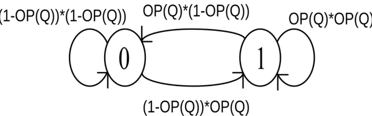
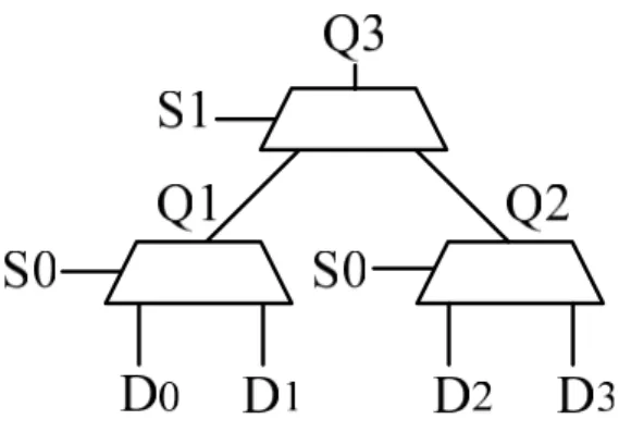
(13) conditions for the 2-to-1 MUX in Fig. 1. The output Q switches as the output Q is from logic 0 to logic 1 or from logic 1 to logic 0. We can observe that the switching activity α of MUX output Q is equal to 2*OP(Q)*(1-OP(Q)). Therefore, the power dissipation of 2-to-1 MUX solely depends on the OP of the MUX output.. (1-OP(Q))*(1-OP(Q)) OP(Q)*(1-OP(Q)). OP(Q)*OP(Q). (1-OP(Q))*OP(Q) Fig. 2. Probabilities of output Q conditions. To analyze the power dissipation of a 2-to-1 MUX, it is essential to compute the OP of the MUX output. For a 2-to-1 MUX in Fig. 1, the OP of MUX output Q is computed by the following equation: OP(Q) = (1 – OP(S)) * OP(D0) + OP(S) * OP(D1). (2). Further, we should analyze the power dissipations of each 2-to-1 MUX in a MUX tree. That is, we should compute the OP of 2-to-1 MUXes in a MUX tree. Also, we just use the OP of data signals, and the OP of selection signals. In Fig. 3, the OP(D0), OP(D1), OP(D2), OP(D3) and OP(S0) are given. According to Equation(2) , we can compute OP(Q1) and OP(Q2). It is easy to see that we can utilize OP(Q1), OP(Q2), and OP(S1) to compute the OP(Q3) by using Equation(2). Therefore, given the OP of data signals and the OP of selection signals, we can use the bottom up approach to analyze the power dissipations of 2-to-1 MUXes in a MUX tree. 4.

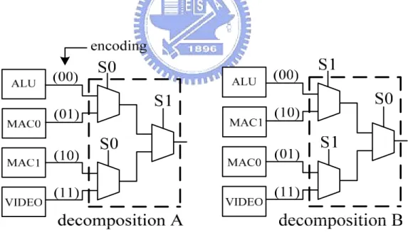
(14) Fig. 3.A 4-to-1 MUX tree. 2.2 MUX Decomposition MUX decomposition is the procedure of transforming an n-to-1 MUX into an equivalent tree of 2-to-1 MUXes. For example, Fig. 4 shows two different decompositions of a 4-to-1 MUX .. original MUX. decomposition A. decomposition B. Fig. 4. Two different decompositions of a 4-to-1 MUX. In Fig. 4, the data signals of the 4-to-1 MUX are denoted by D0, D1, D2, D3 while the selection signals of the 4-to-1 MUX are denoted by S0, S1. The combinations 5.

(15) (S1, S0) of selection signals are used to select one of four data signals to be the 4-to-1 MUX output. We refer to this combination as the encoding for the data signals. For example, the combination (1,1) is used to select D3 to be the MUX output. (S1,S0) = (1,1) is the encoding of D3. Due to the different orders of selection signals for data signals, the original MUX can be transformed to be two different decompositions. Moreover, we can observe that each 2-to-1 MUX in two decompositions are given the different data signals and the different selection signals. According to Equation(2), the different decompositions result in the different power dissipations.. 6.

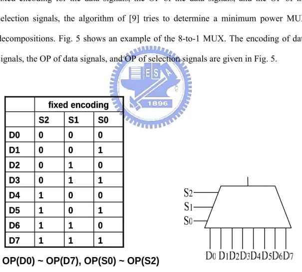
(16) Chapter 3 Previous Works In this chapter, we introduce the previous work [9]. In the first section, we describe the problem formulation of the previous works. In the second section, the bottom up heuristic algorithm proposed in [9] is introduced. In the third section, we give a summary of the bottom up heuristic algorithm.. 3.1 Problem Formulation of the Previous Works [9] The previous work[9] solves the following problem: Given an n-to-1 MUX with a fixed encoding for the data signals, the OP of the data signals, and the OP of the selection signals, the algorithm of [9] tries to determine a minimum power MUX decompositions. Fig. 5 shows an example of the 8-to-1 MUX. The encoding of data signals, the OP of data signals, and OP of selection signals are given in Fig. 5.. fixed encoding S2. S1. S0. D0. 0. 0. 0. D1. 0. 0. 1. D2. 0. 1. 0. D3. 0. 1. 1. D4. 1. 0. 0. D5. 1. 0. 1. D6. 1. 1. 0. D7. 1. 1. 1. OP(D0) ~ OP(D7), OP(S0) ~ OP(S2) Fig. 5. An example of the 8-to-1 MUX. 7.

(17) 3.2 Bottom Up Heuristic Algorithm In the bottom up heuristic algorithm, we construct the MUX decomposition from the bottom level of the MUX tree to the top level of the MUX tree. Fig. 6 shows the first pass of the 8-to-1 MUX. Three cases are formed by choosing three different selection signals as the current selection signal. According to Eauqtion(2), we can observe that the different selection signals cause different power dissipations for each 2-to-1 MUX. In the bottom up heuristic algorithm, we should calculate the sum of power dissipations of the 2-to-1 MUXes. Then, we greedily choose the selection signal with the smallest sum of the calculated power dissipations. For this example, we choose selection signal S0 to be the selection signal of the bottom level due to the smallest sum of the total power dissipations in case1.. first pass:. case1: selection signal S0. case2: selection signal S1. case3: selection signal S2 Fig. 6. First pass of the 8-to-1 MUX. 8.

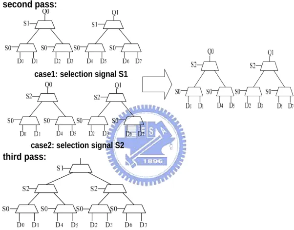
(18) Intuitively, we apply the method of the first pass to choose the selection signals of other levels of MUX tree iteratively. Fig.7 shows the second pass and third pass of the 8-to-1 MUX. In Fig. 7, we greedily choose the selection signals S2 to be the selection signal at the second pass. At the third pass, only selection signal S1 is left to be the selection signal for the top level of MUX tree.. second pass:. case1: selection signal S1. case2: selection signal S2. third pass:. Fig. 7. Second pass and third pass of the 8-to-1 MUX. 9.

(19) 3.3 Summary of Bottom Up Heuristic Algorithm In this section, we give a summary of the bottom up heuristic algorithm. First, the advantage of the bottom up heuristic algorithm is that at each pass we minimize the power of half the remaining 2-to-1 MUXes in a MUX tree. For example, it needs seven 2-to-1 MUXes to construct a 8-to-1 MUX tree. We minimize four 2-to-1 MUXes at the first pass in the bottom up heuristic algorithm. Second, the bottom up heuristic algorithm is an efficient approach to determine a power-minimized MUX decomposition. It returns a solution that is an optimal or near optimal decomposition. We analyze the time complexity of the bottom up heuristic algorithm. If number of data signals is n, the required iterations of bottom up heuristic algorithm is (log2 n) * (log2 n + 1) / 2 - 1.. 10.

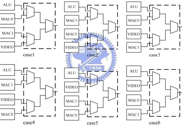
(20) Chapter 4 Motivation In this Chapter, the difference in solution space between the fixed encoding and unfixing encoding for data signals is presented in the first section. In the second section, we analyze the exact number of solutions for the two different solution spaces.. 4.1 Limited Solution Space In selection 2.2, the MUX decomposition has been introduced. An example of two different decompositions is shown in Fig. 8. ALU, MAC0, MAC1, VIDEO are functional blocks. The 4-to-1 MUX is decomposed as a tree of 2-to-1 MUXes. Because the encoding are specified for the outputs of those functional blocks, we reorder the selection signals to explore at most two combinations of decompositions.. Fig. 8. An example of two different decompositions. However, if the encoding for the outputs of those functional blocks is not specified in advance, the outputs of those functional blocks can be assigned to arbitrary input positions of the 4-to-1 MUX. Fig. 9 shows an example of six possible combinations 11.

(21) of those functional blocks. As the encoding is not specified for the outputs of those functional blocks, six possible combinations of those functional blocks can be explored. The decomposition A and the decomposition B in Fig. 8 are the same as case1 and case2 in Fig. 9. Therefore, the solution space of unfixed encoding for data signals is larger than the solution space of fixed encoding for data signals in advance. Actually, each encoding of data signals is specified by designers. The fixed encoding for data signals in advance is not generally necessary.. Fig. 9. An example of six possible combinations of those functional blocks. 4.2 Solution Space Analysis Assume the number of data signals is n. We analyze the exact number of the solutions if the fixed encoding is assigned for data signals. We can reorder the selection signals to search all possible decompositions. Hence, the number of the solutions is (log2 n)!. As the encoding is not specified for data signals in advance, we 12.

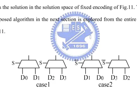
(22) can assign input position of the MUX arbitrary data signals. The number of the possible combinations of the data signals is n!. In Fig. 10, the combination of the data signals in case2 is generated by reversing selection signal S in case1. As well, the power dissipation of case1 is equal to the power dissipation of case2. That is, the number of the solutions should be divided by 2 for each level of the MUX tree. Hence, as encoding is not specified for data signals, the number of the solutions is (n-1)!. The entire solution space is shown in Fig. 11. The solution space of the unfixed encoding is equal to the entire solution space. Additionally, as the number of the data signals increases, the ratio of the solution space of the fixed encoding to the entire solution space decreases significantly. The bottom up heuristic algorithm in [9] searches the solution in the solution space of fixed encoding of Fig.11. The solution of our proposed algorithm in the next section is explored from the entire solution space of Fig. 11.. Fig. 10. Equal power dissipation in both cases. Fig. 11. Entire solution space 13.

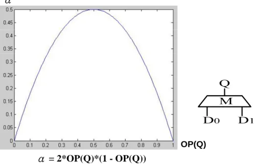
(23) Chapter 5 Proposed Algorithm In this Chapter, we describe the problem formulation of our proposed algorithm in the first section. In the second section, we give a detailed description of our proposed algorithm. In the third section, we summarize our proposed algorithm.. 5.1 Problem Formulation of Proposed Algorithm Our proposed algorithm tries to search a larger solution space than the bottom up heuristic algorithm, so different problem formulation is given. We solve the problem as following: Given the on probabilities (OP) of the data signals and the selection probabilities (SP) of the data signals, our proposed algorithm determines input positions for the data signals in a MUX tree. That is, the proposed algorithm assigns input selection encoding for data signals. According to the input selection encoding of the data signals, a power-minimized MUX tree is generated.. 5.2 Proposed Algorithm In this selection, we give a detailed description of our proposed algorithm.. 5.2.1 Analysis of OP of MUX Output The way to reduce the power dissipation of the MUX is to minimize the switch activity α of the MUX output. The α of the MUX output only depends on the OP of the MUX inputs. We discuss the relation between α and OP of the MUX further. Consider a 2-to-1 MUX and the switching activity curve shown in Fig. 12. The curve represents the equation α = 2*OP(Q)*(1 - OP(Q)). As the OP(Q) is away from 0.5, the α decreases. If we want to reduce power dissipation of the 2-to-1 MUX, we should avoid the OP of the 2-to-1 MUX output approaching 0.5.. 14.

(24) α. OP(Q). α = 2*OP(Q)*(1 - OP(Q)) Fig. 12. A 2-to-1 MUX and switching activity curve. The OP of the 2-to-1 MUX outputs can be computed by Equation(2) and the Equation(2) is actually an interpolation. A 2-to-1 MUX and illustration of Equation(2) are shown in Fig. 13. From the illustration of Equation(2) in Fig. 13, we make two observations. First, OP(Q) is bound between OP(D1) and OP(D0). Second, the position of OP(Q) between OP(D1) and OP(D0) is proportional to the position of OP(S) between 0 and 1.. Fig. 13. A 2-to-1 MUX and illustration of Equation(2). 15.

(25) 5.2.2 2-to-1 MUX Inputs In our proposed algorithm, we construct a MUX tree from the bottom level of MUX tree to the top level of MUX tree. We should minimize the power dissipation of 2-to-1 MUX at a level of MUX tree first. According to Equation(2), if we consider both SP and OP of data signals, the entire solution space must be explored exhaustively. Due to time complexity, an efficient approach must be applied. In section 5.2.1, we have mentioned that the OP of the 2-to-1 MUX output is bound between two OP of 2-to-1 MUX inputs. If we determine 2-to-1 MUX inputs only by considering the OP of data signals, the OP of 2-to-1 MUX output must vary between two OP of the MUX inputs. For example, if we avoid 0.5 between two OP of the 2-to-1 MUX inputs, the OP of the 2-to-1 MUX output could be far from 0.5.Thus, we only consider the OP of the data signals first in our proposed algorithm. Consider an example of different 2-to-1 MUX inputs shown in Fig. 14. Because we consider the OP of the data signals only, we assign four data signals with equal SP to the 2-to-1 MUX inputs in Fig. 14. The data signals with equal SP cause OP(S) to be 0.5, so the OP of the 2-to-1 MUX output is equal to the middle between two OP of the 2-to-1 MUX inputs. In case1 of Fig. 14, we see that the OP(Q1) is in the middle between OP(D0) and OP(D3), so OP(Q1) is 0.5. We also can see that the OP(Q2) is 0.5. In case2 of Fig. 14, the OP(Q1) is 0.15 and the OP(Q2) is 0.75. The sum of α in case1 is higher than the sum of α in case2. From case2, we can instinctively think that if the two data signals which both always have “on” conditions or both have “off” conditions are in the same 2-to-1 MUX inputs, the α of the 2-to-1 MUX output is low. Moreover, we can observe that the OP of the 2-to-1 MUX inputs in case2 avoid the OP of the 2-to-1 MUX outputs approaching 0.5. Thus, if we use 0.5 to partition the OP of the data signals into two groups and the data signals in the same group should 16.

(26) be in the same 2-to-1 MUX inputs, the OP of the 2-to-1 MUX outputs could be far from 0.5.. Fig. 14. An example of different 2-to-1 MUX inputs 17.

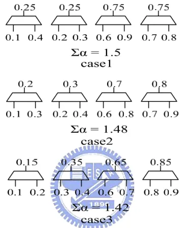
(27) However, only partitioning the data signals into two groups is not enough to determine all of 2-to-1 MUX inputs. We should find an efficient way to determine 2-to-1 MUX inputs in the n-to-1 MUX. Take the 8-to-1 MUX as example. An example of the different 2-to1 MUX inputs in the bottom level of the 8-to-1 MUX is shown in Fig. 15. The table presents the OP and SP of data signals. In the three cases, the data signals in the same group are in the same 2-to-1 MUX inputs. We can see that the sum of α in case3 is smallest among three cases. The approach of case3 uses the sorting order of the OP of the data signals to determine the 2-to-1 MUX inputs. In our proposed algorithm, we greedily adopt the approach of case3 to determine the 2-to-1 MUX inputs. If it has even number of the data signals in both groups, we also use the sorting order to determine 2-to-1 MUX inputs. Thus, our proposed algorithm can efficiently determine 2-to-1 MUX inputs by using sorting order of the OP of the data signals.. 18.

(28) data signals: OP 0.1 0.2 0.3 0.4 0.6 0.7 0.8 0.9 SP 1/8 1/8 1/8 1/8 1/8 1/8 1/8 1/8. Fig. 15. An example of the different 2-to1 MUX inputs in the bottom level of the 8-to-1 MUX. 19.

(29) 5.2.3 Order of 2-to-1 MUX Inputs Although our proposed algorithm determines 2-to-1 MUX inputs, the OP of the 2-to-1 MUX outputs are just bound between two OP of 2-to-1 MUX inputs. From section 5.2.1, the OP of selection probability can determine the position of the OP of the 2-to-1 MUX outputs between two OP of 2-to-1 MUX inputs. The Fig. 16 shows different orders of 2-to-1 MUX inputs. The different orders of 2-to-1 MUX inputs cause the different OP of the selection signal. If we want to determine minimum power of 2-to-1 MUXes by changing the orders of the 2-to-1 MUX inputs, the solution space is too large. For example, if the number of the data signals is n, the number of all combinations of the data signals is 2. (n / 2). .. The example of the equal power dissipation condition is shown in Fig. 10. The number of all combinations of the data signals should be divided by 2. Thus, the total number of the solutions is 2 (n / 2) – 1. Due to time complexity, an efficient way must be proposed.. Fig. 16. Different orders of 2-to-1 MUX inputs. 20.

(30) The OP of the 2-to-1 MUX outputs should be as far from 0.5 as possible. Assume that the 2-to-1 MUX inputs have the following ideal condition: the OP of the 2-to-1 MUX input port “1” is further from 0.5 than the OP of the 2- to-1 MUX input port “0” and 2-to-1 MUX input port “1” has high selection probability. From illustration of Equation(2) in Fig.13, the OP of the 2-to-1 MUX output approaches the OP of the 2-to-1 MUX input port “1” and have low α. Fig. 17 shows the ideal condition of 2-to-1 MUX inputs. In Fig. 17, the OP of the 2-to-1 MUX input port “1” is further from 0.5 than the OP of the 2-to-1 MUX input port “0”. Moreover, the SP of the 2-to-1 MUX input port “1” is higher than the SP of the 2-to-1 MUX input port “0”. Because OP(S) is 0.8, OP(Q1) approaches 0.9 between 0.5 and 0.9, OP(Q2) approaches 0.1 between 0.1 and 0.5. Thus, if the condition of 2-to-1 MUX inputs is the same as the ideal condition of 2-to-1 MUX inputs in Fig. 17, the higher SP of the 2-to-1 MUX input should be in the same input port. Then, the OP of the 2-to-1 MUX output approaches the OP of the MUX input which is further from 0.5 than another. However, we can’t expect that all conditions of the 2-to-1 MUX inputs are the same as the ideal condition of the 2-to-1 MUX input pair in Fig. 17.. Fig. 17. Ideal condition of 2-to-1 MUX inputs. 21.

(31) Next, we classify 2-to-1 MUX input pair into two types form the OP and the SP of the 2-to-1 MUX inputs. The two types of 2-to-1 MUX input pairs are referred as the ideal MUX and the unpredictable MUX. If the condition of the 2-to-1 MUX inputs is the same as the ideal condition of the 2-to-1 MUX inputs in Fig. 17, the 2-to-1 MUX is an ideal MUX. Fig. 18 shows an example of the ideal MUX. We can see that SP(D) > SP(C) and OP(D) < OP(C) < 0.5. The MUX M2 is an ideal MUX. The MUX M2 of case2 has correct order of MUX inputs. The OP(Q1) and the OP(Q2) of case2 are further from 0.5 than the OP(Q1) and the OP(Q2) of case1.The order of the ideal MUX can be determined by the SP and OP of the ideal MUX inputs. Thus, the orders of the ideal MUX inputs can be fixed efficiently without considering other orders of MUX inputs.. A. B. C. D. OP. 0.6. 0.8. 0.4. 0.2. SP. 0.2. 0.3. 0.1. 0.4. case1. case2. OP(Q1) = 0.68, OP(Q2) = 0.28. OP(Q1) = 0.74, OP(Q2) = 0.26. Fig. 18. An example of the ideal MUX. The unpredictable MUX is described as following: the OP of the 2-to-1 MUX input port “1” is further from 0.5 than the OP of the 2- to-1 MUX input port “0” and the SP of the 2-to-1 MUX input port “1” is lower than the OP of the 2- to-1 MUX input port “0”. An example of the unpredictable MUX is shown in Fig. 19. The MUX 22.

(32) M2 is the unpredictable MUX. The OP(Q1) of case2 is further 0.5 than the OP(Q1) of case1. However, the OP(Q2) of case1 is further 0.5 than the OP(Q2) of case2. Both results must be computed to determine the order of the unpredictable MUX inputs. Thus we can’t predict the order of the unpredictable MUX inputs only from the SP and the OP of the unpredictable MUX inputs.. A. B. C. D. OP. 0.6. 0.8. 0.4. 0.2. SP. 0.2. 0.3. 0.4. 0.1. case1 OP(S) = 0.4 OP(Q1) = 0.68, OP(Q2) = 0.32. case2 OP(S) = 0.7 OP(Q1) = 0.74, OP(Q2) = 0.34. Fig. 19. An example of the unpredictable MUX. The properties of both ideal MUX and unpredictable MUX have been introduced. All of 2-to-1 MUXes belong to either the ideal MUX or the unpredictable MUX. All cases of the ideal MUX are shown in Fig. 20. And, two ideal MUX inputs conform the following equation: { |OP(A) - 0.5| ≧ |OP(B) - 0.5| } & { SP(A) ≧ SP(B) }. (3). All cases of the unpredictable MUX are shown in Fig. 21. And, two unpredictable MUX inputs conform the following equation: { |OP(A) - 0.5| ＞ |OP(B) - 0.5| } & { SP(A) ＜ SP(B) } 23. (4).

(33) Fig. 20. All cases of the ideal MUX. 24.

(34) Fig. 21. All cases of the unpredictable MUX. 25.

(35) 5.2.4 Process of Fixing Order of MUX Inputs After the 2-to-1 MUX inputs are given, we should find an efficient approach to fix orders of the 2-to-1 MUX inputs to minimize α of the MUX outputs in our proposed algorithm. First, we find all of the ideal MUXes and fix orders of the ideal MUX inputs. Fig. 22 shows the process of fixing orders of ideal MUX inputs.. Fig.22. Process of fixing orders of ideal MUX inputs. We can’t expect that all 2-to-1 MUXes are the ideal MUXes. After fixing the orders of the ideal MUX inputs, we have to fix the orders of the unpredictable MUX inputs. Due to time complexity, we can’t search all possible solutions exhaustively by swapping the unpredictable MUX inputs. According to Equation(2) and Equation(3), only the SP of the data signals affect the OP of the 2-to-1 MUX outputs after the 2-to-1 MUX inputs are given. Consequently, we greedily fix the order of the unpredictable MUX first which has the largest sum of the two SP of the unpredictable MUX inputs. The process of fixing orders of the unpredictable MUX inputs is shown in Fig. 24. The MUX M1 and the MUX M2 are the ideal MUXes, and their orders have been fixed. The MUX M3 and the MUX M4 are the unpredictable MUXes. The sum of the SP(E) and the SP(F) is larger than the sum of SP(G) and SP(H), so we fix the order of MUX M3 inputs first. As computing the OP(S), the only fixed MUX are considered. The different orders of the MUX M3 inputs cause the different OP(S). The total power dissipation is the sum of the Q1, Q2, and Q3. We compute the two 26.

(36) different total power dissipations. Then we greedily choose the order of the MUX inputs which generates the lowest total power dissipation. In this example, the total power dissipation of case2 is lower than the total power dissipations of case1. Thus, the order of MUX M3 inputs of case2 is chosen. We use the same approach to fix all orders of the unpredictable MUX inputs iteratively. After fixing all orders of the unpredictable MUX inputs, the input positions of the data signals in a level of the MUX tree are determined.. OP(S)=. SP(B)+SP(D)+SP(F) SP(A)+SP(B)+SP(C)+SP(D)+SP(E)+SP(F). OP(S)=. SP(B)+SP(D)+SP(E) SP(A)+SP(B)+SP(C)+SP(D)+SP(E)+SP(F). Fig.24. Process of fixing orders of the unpredictable MUX inputs. In our proposed algorithm, we construct a MUX tree from the bottom level to the top level. From the previous steps, we have analyzed how to determine the input positions of the data signals in a level of the MUX tree. Then we can obtain the OP of the each 2-to-1 MUX output in a level of the MUX tree. It is easy to see that the SP of the 2-to-1 MUX output is the sum of the SP of the 2-to-1 MUX inputs. By using the 27.

(37) SP and the OP of the MUX outputs in a level of the MUX tree, we use the same approach to determine next level of a MUX tree. Finally, the input positions of the data signals in a MUX tree are determined. That is, input selection encoding is assigned to the data signals.. 5.3 Summary of Proposed Algorithm According to the main idea introduced in previous sections, the process of our proposed algorithm can be summarized in the following steps: ● Determine 2-to-1 MUX inputs in a level of the MUX tree greedily by using the sorting order of the OP of the data signals. ● Classify the 2-to-1 MUX inputs into two types from the SP and the OP of the 2-to-1 MUX inputs. The two types are the ideal MUX and the unpredictable MUX . ● Fix the orders of the ideal MUX inputs first. For example, all of the ideal MUX input port“1” are given 2-to-1 MUX input which has higher SP than another input. ● Fix the orders of the unpredictable MUX inputs one by one. The priority is given by the sum of the two SP of the unpredictable MUX inputs. ● After the orders of the 2-to-1 MUX inputs are fixed in the a level of the MUX tree, the SP and the OP of the 2-to-1 MUX outputs are known. Thus, apply the previous steps to determine each level of the MUX tree iteratively. ● Finally, the input positions of the data signals in a MUX tree are determined and the input selection encoding is assigned for the data signals.. 28.

(38) Chapter 6 Experimental Results and Analysis We implement both bottom up heuristic algorithm and our proposed algorithm in our experiments. We apply these algorithms on 4-to-1, 8-to-1, 16-to-1, 32-to-1, and 64-to-1 MUXes. The implementations are in C++. The different OP and SP of the data signals cause the different results. We randomly generate 100 different cases of the OP and the SP for data signals when we apply these algorithms on each n-to-1 MUX. Then, we recorder those results and get the average result. We define that the better solution is the solution which is better than the reference solution in the entire solution space. Table 2 shows the average number of the better solutions in the 4-to-1 MUX. Table 3 shows the number of the better solutions in the 8-to-1 MUX. The “average solution” is the average result of 1000 random cases for different data signals. The better case ratio is calculated by the following equation: better solution ratio =. number of average better solutions number of total solutions. (5). The number of the total solutions is 3! = 6 for a 4-to-1 MUX. The number of the total solutions is 7! = 5040 for an 8-to-1 MUX. The “variance” presents the variance of average number of better solutions. The variance is not great in 4-to-1 MUX and 8-to-1 MUX. The solutions of bottom up heuristic algorithm are near best solutions of MUX decomposition. However, about 20% of the total solutions are better than the best solution of MUX decomposition in 8-to-1 MUX due to small solution space. The solution of our proposed algorithm is better than over 95% of the total solutions in 8-to-1 MUX. If the size of the MUX is over 8, the total solution space is too large. We only search the total solutions of the both 4-to-1 MUX and 8-to-1 MUX to compare results.. 29.

(39) Table 1. Average number of the better solutions in the 4-to-1 MUX. approach. average solution. Liu’s work. best solution of MUX decomposition. Proposed. average number of better solutions. 2.97. 1.96. 1.96. 0.39. variance. 0.82. 0.73. 0.73. 0.75. better solution ratio. 49.50%. 32.67%. 32.67%. 6.50%. Table 2. Average number of the better solutions in the 8-to-1 MUX. approach. average solution. Liu’s work. best solution of MUX decomposition. proposed. average number of better solutions. 2451.58. 1031.72. 926.87. 28.13. variance. 138.85. 220.79. 187.15. 46.06. better solution ratio. 48.64%. 20.47%. 18.39%. 0.56%. The total solutions of the arbitrary n-to-1 MUX can’t be obtained. We analyze the results by using the following equation: power saving rate =. average solution - reference soultion average solution. 30. (6).

(40) Moreover, we observe the each power saving rate at different ranges of OP of the data signals. The three different ranges are {0< OP <1}, {0.2 < OP < 0.8}, and {0.4 < OP < 0.6}. The power saving rates at the three different ranges is shown in Table 3, Table 4, and Table 5. The solutions of the proposed algorithm are near the best solutions of entire solution space in the 4-to-1 MUX and 8-to-1 MUX. In our proposed algorithm, as the size of the MUX increases, the power saving rate increases. For example, the power saving rate of 64-to-1 MUX is up to about 24% at the range {0 < OP <1}. In the bottom up heuristic algorithm, as the size of the MUX increases, the power saving rate decreases. This is because that the ratio of the solution space of MUX decomposition to the entire solution space decreases significantly, as the size of the MUX increases. From Table 3, Table 4, and Table 5, the power saving rate decreases as range of the OP diminishes. From Equation(4), if the OP of the data signals is between 0.4 and 0.6, the OP of the MUX outputs still vary between 0.4 and 0.6 with any combinations of the data signals. Thus, the range of the OP of data signals limits the power saving rate.. Table 3. Power saving rate at the range {0 < OP < 1} Liu’s work. best solution of MUX decomposition. proposed. best solution of entire solution space. 4-to-1 MUX. 4.46%. 4.46%. 7.82%. 9.36%. 8-to-1 MUX. 5.56%. 6.03%. 16.78%. 18.75%. 16-to-1 MUX. 5.26%. 5.74%. 20.89%. _. 32-to-1 MUX. 4.50%. 4.83%. 23.43%. _. 64-to-1 MUX. 3.19%. 3.38%. 24.33%. _. 31.

(41) Table 4. Power saving rate at the range {0.2 < OP < 0.8}. Liu’s work. best solution of MUX decomposition. proposed. best solution of total solution space. 4-to-1 MUX. 1.28%. 1.28%. 2.65%. 3.00%. 8-to-1 MUX. 1.88%. 2.06%. 5.48%. 6.18%. 16-to-1 MUX. 1.76%. 1.89%. 6.72%. _. 32-to-1 MUX. 1.49%. 1.60%. 7.75%. _. 64-to-1 MUX. 1.22%. 1.28%. 8.10%. _. Table 5. Power saving rate at the range {0.4 < OP < 0.6}. Liu’s work. best solution of MUX decomposition. proposed. best solution of total solution space. 4-to-1 MUX. 0.12%. 0.12%. 0.30%. 0.32%. 8-to-1 MUX. 0.19%. 0.20%. 0.59%. 0.67%. 16-to-1 MUX. 0.19%. 0.20%. 0.78%. _. 32-to-1 MUX. 0.16%. 0.18%. 0.83%. _. 64-to-1 MUX. 0.14%. 0.14%. 0.86%. _. 32.

(42) Chapter 7 Conclusions and Future Works In this thesis we have solved the following problem: Given the SP and OP of the data signals, our proposed algorithm determine input positions for the data signals in a MUX tree. That is, the input selection encoding is assigned for the data signals. According to the input selection encoding of the data signals, a power-minimized MUX tree is generated. We analyze the differences in solution space between fixed encoding and unfixed encoding for the data signals. Because the fixed encoding for data signals limits the size of the solution space, our proposed algorithm is applied without fixed encoding for data signals. From experimental results, the solution of our proposed algorithm is better than over 90% of total solutions in 4-to-1 MUX and 8-to-1 MUX. Moreover, as the number of the data signals increases, the power saving rate increases in the proposed algorithm. For example, the power saving rate is 24% for 64-to-1 MUX at the OP range between 0 and 1. Our proposed algorithm only considers the n-to-1 MUX where n is power of 2. The incomplete MUX where size of MUX is not power of 2 is not adoptable in our proposed algorithm so far. There are two problems. First, our proposed algorithm can’t handle the odd number of the data signals, because one data signal is not assigned to 2-to-1 MUX inputs. Second, some solution space can’t be explored. For example, if the number of data signals is six, there are eight input positions for the six data signals. Our proposed algorithm always assigns the six data signals to six continuous input positions. And, the combination of non-continuous input positions can’t be explored. Thus, in future works, we should extend our approach to handle incomplete MUX tree or we use other algorithms to determine a minimum power incomplete MUX tree.. 33.

(43) References [1] V. Tiwari, P. Ashar, and S. Malik, “Technology mapping for low power”, Design Automation Conference, pp 74-79, June 1993. [2] Shashidhar Thakur, D. F. Wong, and Shankar Krishnamoorthy, “Delay minimal decomposition of mulitiplexers in technology mapping,” Desgin Automation Conference, 1996. [3] A. Ghosh, “Estimation of average switching activity in combination and sequential circuits,” Proc. 29 th DAC, pp 253-259, June 1992. [4] Rajeev Murgai, Robert K. Brayton, and Alberto Sangiovanni-Vincentelli, “Decomposition of logic functions for minimum transition activity,” Proceedings of European Design and Test conference, pp 404-410, 1995. [5] A. Chandrakasan, R. Brodersen, “Minimizing power consumption in digital CMOS circuits,” IEEE Proceedings, vol. 83, no. 4, pp. 473-484, April 1996. [6] Unni Naray anan, P eic hen Ran, and C. L. Liu, “Low power logic synthesis under a general delay model”, Proceedings of International Symposium on Low Power Electronics Design, pp. 209-214. 1998. [7] Chi-Ying Tsui, Massoud Pedram, and Alvin M. Despain, “Technology decomposition and mapping targeting low power dissipation”, Design Automation Conference, pp 68-73, 1993. [8] Eric Lehman, Yosinori Watanabe, Joel Grodstein, and Heather Harkness, “Logic decomposition during technology mapping,” International Conference on Computer-Aided Design, pp 264-271, 1995. [9] Unni Narayanan, Hon Wai Leong, Ki-Seok Chaung, and C.L.Liu, “Low power Multiplexer Decomposition,” Proceedings of International Symposium on Low Power Electronics Design, pp. 269-274. 1997. 34.

(44) [10] Kisun Kim, Taekyoon Ahn, Sang-Yeol Han, Chang-Seung Kim, and Ki-Hyun Kim, “Low-power multiplexer decomposition by suppressing propagation of signal transitions,” Circuits and Systems, vol.5, no.5, pp 85-88, May 2001.. 35.

(45)