模糊樣本資料之新統計檢定程序與決策

行政院國家科學委員會專題研究計畫 成果報告

模糊樣本資料之新統計檢定程序與決策(第 3 年)

研究成果報告(完整版)

計 畫 類 別 ： 個別型 計 畫 編 號 ： NSC 96-2416-H-004-014-MY3 執 行 期 間 ： 98 年 08 月 01 日至 99 年 07 月 31 日 執 行 單 位 ： 國立政治大學應用數學學系 計 畫 主 持 人 ： 吳柏林 報 告 附 件 ： 出席國際會議研究心得報告及發表論文 處 理 方 式 ： 本計畫涉及專利或其他智慧財產權，1 年後可公開查詢

中 華 民 國 99 年 09 月 30 日

行政院國家科學委員會補助專題研究計畫

■ 成 果 報 告

□期中進度報告

模糊樣本資料之新統計檢定程序與決策

計畫類別：■個別型計畫 □整合型計畫

計畫編號：

NSC962416H004014-MY3

執行期間：96 年 8 月 1 日至 99 年 7 月 31 日

執行機構及系所: 政大應數系

計畫主持人：吳柏林

共同主持人：

計畫參與人員：

成果報告類型(依經費核定清單規定繳交)：□精簡報告 ■完整報告

本計畫除繳交成果報告外，另須繳交以下出國心得報告：

□赴國外出差或研習心得報告

□赴大陸地區出差或研習心得報告

■出席國際學術會議心得報告

□國際合作研究計畫國外研究報告

處理方式：

除列管計畫及下列情形者外，得立即公開查詢

□涉及專利或其他智慧財產權，□一年□二年後可公開查詢

中 華 民 國 99 年 8 月 1 日

附件一

1. Introduction

Point forecasting gives important information during decision-making processes, especially on economic developments, population policies, management planning or financial controls. Nevertheless, its drawbacks still include: (1) it is not efficient in the marketing application due to the inaccurate forecasting; (2) the model constructed only by the closing price may not illustrate the whole process of daily or monthly trend. The causes of this regretful situation are that the business marketing is full of uncertainty and human being’s manipulation. In this paper, we proposes interval forecasting approaches, such as the interval moving average, the weighted interval moving average, and ARIMA interval forecasting. We generate interval time series by simulation and apply the proposed forecasting approaches to carry out the interval forecasting. The forecast results are compared by the mean squared interval error and the mean relative interval error. Finally, we take the monthly trading prices of China Steel stock as a case study. In the comparison of forecasting performance, it is found that ARIMA interval forecasting provides more efficiency and flexibility than the traditional ones do.

In the forecasting and analysis of time series, the tendency of the data interval is paid more and more attention, such as daily temperature changes, the fluctuation of the exchange rate, the level price of petroleum etc. According to the characteristic of observed data, traditional time series analysis selects the best fitted model from a priori models, such as ARIMA model, ARCH model or the threshold model etc. Due to the uncertainty of the predicted points, intervals are used as the estimated prediction values. Montgomery and Johnson (1976), Abraham and Ledolter (1983), Chatfield (1989) proposed prediction interval by time series of points to carry out the prediction.

Based on different factors and data types, there are a diversity of prediction methods. Chatfield (1993) made a comparison of several different methods. And Diebold and Mariano (1995) proposed the discussion in the respect that different prediction methods have their own pros and cons depending on the time series has a steady tendency or a severe fluctuation. Christoffersen (1998) provided the calculation method of interval forecasting for the risk measurement. Despite there are various methods of interval forecasting due to the variety of the backgrounds and the purposes of research, the data collections are mostly in the basic form of single real numerical variable. Even though there are many interval prediction methods, Chatfield (1996) pointed out that the prediction intervals resulted by those methods are too narrow owing to a lot of factors, one of which is the problem whether the model is appropriate.

This paper proposes the interval forecasting that uses interval time series to carry out the prediction and analysis of intervals, whereas actually the literature of dynamic data analysis applied to interval data is few. We employ the methods of AR(1) and ARCH(1) to make multiple simulations on each single time point in order to find the interval of each time point to design four sets of stable or unstable interval time series. Thus, we can proceed the interval forecasting in accordance with the proposed forecasting methods, which are the interval moving average of order k, the weighted interval moving average of order k, ARIMA((pc, dc, qc), (pr, dr, qr)) of (c,r) and ARIMA((pm, dm, qm), (pl, dl, ql), (pu, du, qu)) of (m, l, u).

However, when ARIMA is applied to the analysis of interval time series, the most important step is to consider how to associate the central point and the interval length to make an integrated analysis. Therefore, we denote an interval by the central point and the interval radius instead of the traditional interval expression, complying with the rules of interval operations established by Young (1931) and the properties of the interval algorithm by Dwyer (1951). This paper applies the interval calculation technology to explore the model construction and forecasting of interval time series. First, we must give the appropriate definitions of random interval and its expectation. Then ARIMA is employed to construct the models of the central points and the interval lengths separately. At last, the interval forecasting can be carried out by means of the constructed models.

It is necessary to determine the validity of the forecasting method by means of the estimated error between the predicted data and the simulated data. Chatfield (1996) declared that the error made by an inappropriate interval prediction method is more severe than the error made by a simple point prediction. Therefore, in order to assess the efficiency of interval forecasting, we define several criteria, referring to the traditional efficiency measurements, to evaluate the efficiency of forecasting. We make an integrated analysis of the efficiency by associating the central point and length of the interval, which are the mean squared error

of interval and the mean relative interval error respectively. Finally, regardless of the simulated interval time series or the practical data, using ARIMA to proceed the interval forecasting is more appropriate than using traditional prediction technologies, such as moving average and weighted moving average.

In this paper, we propose the model construction and its theoretical architecture of interval time series analysis and forecasting. We use the monthly highest and lowest prices of stocks as our case study. The mean squared error of interval is taken into account to be compared with the mean of relative interval error to validate the forecasting effect, which will be helpful for the study and judgment on the trend of the future financial market. The interval prediction by interval time series can provide more objective decision space to policymakers.

2. Analysis of Interval Time Series 2.1. The interval data

The traditional social and economic studies have brought in various analyses of interactive relationship and model related to human. In the traditional model construction, we often confront the uncertainty data problem. For instance, should we count the number of yearly enrolled students at the beginning of the year? at midyear? or at the end of the year? The obtained number is often different at different time. For another example, what is the exchange rate of U.S. dollar to Japanese Yen last week? is with the opening quotation? the closing price? or the average of the highest price and the bottom price? The results are also quite different. Wu and Chen (1999) have given an extensive review of literature on this topic. In the social science study or economic research, obviously the answer to these questions is not just true or false. There are lots of uncertain and incomplete information or events so that we can not apply the conventional real number system to process it. In many practical cases under the influences of many factors, the observed data usually appear not only a single numerical value type but also a “range”.

2.2. The operation of interval data

While we consider the data to be of interval type, we must encounter the various problems of interval operations as well as the realistic meanings. Dwyer (1951) called intervals as "range numbers" and defined the relevant operations. The subsequent studies relative to the interval operations continually quote such definitions. Nevertheless, it is still unable to give the standard rules of interval operations on the computer hardware. Hayes (2003) pointed out that the rules of interval operations seem simple, but there often appears a trap of miscalculation in the practical calculations, especially in the case that the element 0 is contained in an interval. The traditional interval operations are given as follows:

[ ] [ ]

a,b _o c,d =

[

min

(

a_oc,a_od,b_oc,b_od

)

,max

(

a_oc,a_od,b_oc,b_od

)

]

,

where o denotes any of ＋, －, × and ÷. That means that the interval operation takes the extreme values of c

a o , _{a o}d, _{b o}c and _{b o}d as the resulted interval. This definition is feasible for addition, subtraction and multiplication. But in the case of division, such interval operation will lead to a blind spot in computation. For example,

[ ] [

3,5 ÷ −1,1

]

will obtain the answer

[

−5,5

]

. But actually 0∈

[

−1,1

]

and

[ ]

3,5 ÷0 is not well defined, so that such the answer

[

−5,5

]

is meaningless.

Furthermore, when we process a set of dynamic data represent by the interval form, we often encounter certain realistic dilemma. For instance, does the value increase or decrease from [2, 8] to [3, 5]? We may consider the location variation between intervals. But if we take the interval scale into considerations, this case becomes more complicated. Hence, in this paper we will propose the bivariate parameters, which are (i) the interval radius to express the interval scale and (ii) the interval center to express the interval location, to demonstrate the variations of intervals. For the above example, the interval location is decreased from 5 to 4, whereas the interval radius is also decreased from 3 to 1. Such a new interval expression, which integrates the interval center with the interval radius, is apt to show the

location shift and the length variation of interval data. By the proposed interval expression, we are able to make an appropriate interval forecasting for the interval time series. And under the assistance of computer programs, even more complicated calculation can be easily solved.

2.3. Definitions and Properties of Interval Time Series

The interval time series is the analytical method to apply intervals to the analysis of time series, incorporating with the interval operations, so as to solve the uncertainty of the data. As a result, before constructing and forecasting the model of interval time series, we must first give several definitions relevant to interval time series. The definition of a random interval defined by Nguyen and Wu (2006) is given in Definition 2.1, and the other relevant definitions are given as follows.

Definition 2.1 (A random interval)

Let X =

[ ]

a,b . If aand b are random variables, then the interval

[ ]

a,b is called a random interval.

Definition 2.2 (A random interval of alternate notation, X =

( )

c,r )

Suppose X=[a, b] be a random interval over the real numbers ℜ, c=(a+b)/2 be the center of the interval X, and r=(b-a)/2 be the radius of the interval X, then the interval X can be expressed as X =( rc, ).

Definition 2.3 (The mean of a random interval X =( rc, ))

Let X =( rc, ) be a random interval over the real numbers ℜ. The mean of the random interval X is defined as E

[ ] [ ]

X =Ec,r =

(

E

[ ] [ ]

c,E r

)

, where E

[ ]

c and E

[ ]

r are the expectations of the random variables c and r respectively.

In some special conditions, we could known there is a value which manipulates the position and the length of the interval X. For example, if the daily highest price of a stock is b, the daily lowest price is a, and the weighted average price is m, then m is not necessarily the median value c. Hence the distances between m and b is different from that between m and a. There is a similar situation in the weather forecast. If the daily average temperature is m, obviously m is not likely the median value of the highest and lowest temperatures. Therefore, m is called the weighted center, defined as follows.

Definition 2.4 (The weighted center of random interval, m)

Let X =

[ ]

a,b be a random interval over the real numbers ℜ. If there is such a value, denoted as m, which influence position and the length of the random interval X, then the value m is called the weighted center of random interval X.

Definition 2.5 (A random interval , X =

(

m,l,u

)

)

Suppose X =

[ ]

a,b is a random interval over the real numbers ℜ. Let m be the weighted center of the interval X, l=m−a and u=b−m be the distances between the weighted center and the boundaries of interval X respectively. Then the interval X can be expressed as X =

(

m,l,u

)

.

Definition 2.6 (The mean of random interval X =

(

m,l,u

)

)

Let X =

(

m;l,u

)

be a random interval over the real numbers ℜ. The mean of the random interval X is defined as E

[ ] [

X =E m,l,u

]

=

(

E

[ ] [ ] [ ]

m,El, u

)

, where E

[ ]

m , E

[ ]

l and E

[ ]

u are the expectations of random

variables m、l and u respectively.

Definition 2.7 (The interval addition)

Let X₁=

[

a₁,b₁

]

=

(

c₁,r₁

)

and X₂ =

[

a₂,b₂

]

=

(

c₂,r₂

)

be random intervals. The interval addition is defined as follows:

Interval addition: X₁⊕X₂ =

(

c₁,r₁

) (

⊕ c₂,r₂

) (

= c₁+c₂,r₁+r₂

)

,

Definition 2.8 (The intervalscalar multiplication)

If X =

[ ] ( )

a,b = c;r is a random interval and k is a scalar, then the scalar multiplication of X by k is the interval given by kX = k

( )

c,r =

(

kc, kr

)

.

From the definition 2.7 and 2.8, the the interval subtraction can be obtained as follows:

(

2

) (

1 1

) (

2 2

) (

1 2 1 2

)

1 2 1 X X X c ,r c ,r c c ,r r X Ο = ⊕ − = ⊕ − = − + . Remark1

1. The interval additive identity is the zero interval: Ο=

[ ]

0,0 =

( )

0,0 . 2. The interval additive inverse: −X =

[

−b,−a

]

=

(

−c,r

)

.

3. The interval absolute value:

( )

( )

( )

( )

⎪ ⎩ ⎪ ⎨ ⎧ ∉ ∈ ⎟⎟ ⎠ ⎞ ⎜⎜ ⎝ ⎛ + + = = . , 0 , , 0 2 , 2 , r c if r c r c if r c r c r c X

Definition 2.9 (The interval length)

Let X =

[ ]

a,b =

( )

c,r be a random interval, the interval length of X is 2r =b−a, and denoted as

r X =2 .

Definition 2.10 (The distance between two intervals)

Let X₁=

[

a₁,b₁

]

=

(

c₁,r₁

)

and X₂ =

[

a₂,b₂

]

=

(

c₂,r₂

)

be two random intervals, then the distance between

1

X and X₂ is defined as D

(

X₁,X₂

)

= X₁ΟX₂ =2

(

r₁+r₂

)

.

Property 2.1

X₁ΟX₂ =0if only if r₁ =0and r₂ =0.

Definition 2.11 (Positive intervals and negative intervals)

Let X =

[ ]

a,b =

( )

c,r be a random interval. If the range of X is all positive, i.e. x≥0 for all x∈X, then X is a positive interval. If the range of X is all negative, i.e. x≤0 for all x∈X, then X is a negative interval.

Definition 2.12 (The interval multiplication)

If X₁ =

[

a₁,b₁

]

=

(

c₁,r₁

)

and X₂ =

[

a₂,b₂

]

=

(

c₂,r₂

)

are two random intervals, the interval multiplication of X1 and X2 is denoted as X1⊗X2.

Because the interval multiplication involves the problems of changing sign and whether zero is in intervals or not, there should consider several situations, described separately as follows.

(Case 1) If 0 does not belong to any of the intervals X1 and X2, and the two intervals X1 and X2 both are

positive intervals or negative intervals, then X₁⊗X₂ =

(

c₁c₂ +r₁r₂,c₁r₂ +c₂r₁

)

.

(Case 2) If the intervals X1 and X2 do not contain 0, and one of them is a positive interval and the other is

a negative interval, then X₁⊗X₂ =

(

c₁c₂ −r₁r₂,c₁r₂−c₂r₁

)

.

(Case 3) If an interval includes 0, there included both positive and negative numbers in the range of the interval. Thus, if either interval contains 0, the calculation of interval multiplication becomes much more complicated. To simplify the problem, let zero be separated from the interval. We can assume

the interval X₁ contains 0 without loss of generality, let

[

1 1

] [

1 1

]

(

1 1

) (

1 1

)

1 2 1 c r,0 0,c r c ,r c ,r A A X = − ∪ + = ′ ′ ⊕ ′′ ′′ = ⊕ , where 2 1 1 1 r c c′= − , 2 1 1 1 r c r′= − , 2 1 1 1 r c c′′= + , 2 1 1 1 r c

r′′= + . Notice A₁ =

(

c₁′,r₁′

)

is a negative interval and A₂=

(

c₁′′,r₁′′

)

is a positive interval. Therefore, the interval multiplication can be expressed as

(

1 2

)

2

(

1 2

) (

2 2

)

2

1 X A A X A X A X

X ⊗ = ⊕ ⊗ = ⊗ ⊕ ⊗ . Then A₁⊗X₂ and A₂⊗X₂ satisfy the conditions in (Case 1) and (Case 2). As a result, the interval mutilplication X1⊗X2 can be obtained by the

interval addition of A₁⊗X₂ and A₂⊗X₂.

(Case 4) If both intervals X1 and X2 contain 0, then X1=A1⊕A2 and X2=B1⊕B2, where A1, B1 are

negative intervals, and A2, B2 are positive intervals. As the same description in (Case 3), the product interval X₁⊗X₂ can be calculated. Because the calculation is much more complex and is not the main issue in this paper, the detail is not discussed here.

Definition 2.14 (Interval time series)

An interval time series is a sequence of random intervals, X_t =

[

a_t,b_t

]

=

(

c_t,r_t

)

, t=1,2,3,_K, denoted as

{ }

X_t =

{

X_t =

[

a_t,b_t

]

=

(

c_t,r_t

)

t=1,2,3,K

}

.

Definition 2.15 (Stationary interval time series of order k)

Let

{ }

X_t be an interval time series. If

(

)

k k r c k t k t X

X ₊ − =∆ = δ ,ε for any t=1,2,3,_K, where E[δ_ck]=δ

and [ε ]=ε

k

r

E , then

{ }

X is called a stationary interval time series. _t

Property 2.2 Let

{ }

X_t =

{

X_t =

[

a_t,b_t

]

=

(

c_t,r_t

)

t=1,2,3,_K

}

be a stationary interval time series, then both

{ }

ct and

{ }

rt are stationary time series.

Example 2.1 Let A = [1, 3] = (2, 1), B = [2, 6] = (4, 2), then

( ) ( ) (

2,1 ⊕ 4,2 = 2+4,1+2

) ( )

= 6,3 = ⊕ B A ,

( ) ( ) (

2,1 − 4, 2 = 2−4,1+2

) (

= −2,3

)

= ΟB A ,

( ) ( )

2,1 ⊗ 4,2 =

(

2⋅4+1⋅2,,2⋅2+4⋅1

)

=

(

10,8

)

= ⊗ B A ,

( ) (

2,1 3 2,3 1

) ( )

6,3 3 3A= = ⋅ ⋅ = .

2.4. The Forecasting Models of Interval Time Series

A traditional time series is defined as

{

X_t =x_t,t=1,2,3,_K

}

, and the corresponding prediction

[

1, 2, , 1

]

ˆ _{E X X X X}

X_t = _{t t− t− K} is a point prediction. The traditional prediction model for traditional time series is not capable of being applied directly to the forecasting of interval time series

[

]

(

)

(1) Interval moving average of order k (IMA) Let k c c c t t k t − − + + = ... ˆ 1 _, k r r rˆ t t k t − − + ⋅⋅ ⋅ +

= 1 _{, t=k+1,k+2,k+3,...., then the forecasting of interval time}

series is E

[

X_t X_t−₁,X_t−₂,K,X_t−_k

]

=

[

cˆ_t −rˆ_t,cˆ_t +rˆ_t

]

=

(

cˆ_t,rˆ_t

)

.

(2) Weighted interval moving average of order k (WIMA)

Let

∑

− − = = 1 ˆ t k t i i i t pc c ,

∑

− − = = 1 ˆ t k t i i i t pr r , for t=k+1,k+2,k+3,_K , where

∑

− − = = _{t 1} k t j j i i f f p , || || || || R X f i i= , for 1 , , 1 , − + − − =t k t k t i _K , and

{ }

{ }

⎥⎦ ⎤ ⎢⎣ ⎡ = − ≤ ≤ − − ≤ ≤ −k j t j t k j t j t a b R 1 1 , max

min , ⋅ denotes the length of an interval. Then

the forecasting of interval time series is E

[

X_t X_t−1,X_t−2,_K,X_t−k

]

=

[

cˆ_t −rˆ_t,cˆ_t +rˆ_t

]

=

(

cˆ_t,rˆ_t

)

. (3) ARIMA((pc, dc, qc), (pr, dr, qr)) of (c, r) interval forecasting (ARIMA IF)

If

{

X_t =

(

c_t,r_t

)

}

is a stationary interval time series, then

{ }

c_t and

{ }

r_t are stationary time series, and

c c c t t q t q p t c p t t c c c =θ+φ_{1 −1}+...+φ ₋ +δ −θ₁δ₋₁−...−θ δ₋ , r q t r q t t p t p t t r rr r r =α+β_{1 −1}+...+β ₋ +ε −η₁ε ₋₁−...−η ε ₋ where _~

( )

_0, 2 c t WN σ δ and _~

( )

_0, 2 r t WN σ ε . Therefore, E

[

ctct−1,ct−2,L,c1

]

=θ+φ1ct−1+...+φp_cct−p_c , and

[

rtrt rt r

]

rt prt p_r E −1, −2,L, 1 =α+β1 −1+...+β _r − .

Let cˆ_t =E

[

c_tc_t−1,c_t−2,_L,c₁

]

and rˆt =E

[

rtrt−1,rt−2,L,r1

]

, then the forecasting of interval time series is

[

Xt Xt Xt X

]

[

ct rt ct rt

]

(

ct rt

)

E ₋₁, ₋₂,..., ₁ = ˆ −ˆ, ˆ +ˆ = ˆ ,ˆ .

(4) ARIMA((pm, dm, qm), (pl, dl, ql), (pu, du, qu)) of (m, l, u) interval forecasting

Let

{

X_t =

(

m_t,l_t,u_t

)

}

be a stationary interval time series, then

{ }

m_t 、

{ }

l_t 及

{ }

u_t are all stationary time series, and

m q t m q t t m p t p t t m m m m − − − − + + + − − − + =θ φ_{1 1} ... φ δ θ₁δ ₁ ... θ δ l l l t p lt lt ql lt q p t t l l l =α+β_{1 −1}+...+β ₋ +ε_, −η₁ε _,−1−...−η ε_,− u u u u t p ut ut q ut q p t t u u u =τ +ω_{1 −1}+...+ω ₋ +ε _, −ϕ₁ε _,−1−...−ϕ ε _,− where ~ (0, 2) m t WN σ δ , ~ (0, 2) ,t l l WN σ ε , and ~ (0, 2) ,t u u WN σ ε . Then

[

mt mt mt m

]

mt p mt p_m E ₋₁, ₋₂,_L, ₁ =θ+φ_{1 −1}+...+φ _{m −} ,

[

lt lt lt l

]

lt p_llt p_l E ₋₁, ₋₂,_L, ₁ =α+β_{1 −1}+_L+β ₋ ,

[

utut ut u

]

ut puut pu E ₋₁, ₋₂,_L, ₁ =τ +ω_{1 −1}+_L+ω ₋ .

And let mˆ_t =E

[

m_tm_t−1,m_t−2,_K,m₁

]

, lˆ_t =E

[

l_t l_t−1,l_t−2,_K,l₁

]

, uˆ_t =E

[

u_tu_t−1,u_t−2,_K,u₁

]

, then the forecasting of interval time series is

[

Xt Xt Xt X

]

[

mt lt mt ut

]

(

mt lt ut

)

E ₋₁, ₋₂,..., ₁ = ˆ −ˆ, ˆ + ˆ = ˆ ,ˆ,ˆ .

Example 2.2 Let

{ }

X_t =

{

[ ] [ ] [ ] [ ] [ ]

1, 2, 2, 4, 3, 4, 4, 6, 3, 7

}

. That is X₁ =

[ ]

1, 2 =

(

1.5,0.5

)

,

[ ]

2,4

( )

3,1

2 = =

X , X₃ =

[ ]

3,4 =

(

3.5,0.5

)

, X₄ =

[ ]

4,6 =

( )

5,1 , and X₅ =

[ ]

3,7 =

( )

5,2 . Then by the interval moving average of order 5, we can obtain

[

]

(

3.6,1

)

[

3.6 1,3.6 1

] [

2.6,4.6

]

. 5 2 1 5 . 0 1 5 . 0 , 5 5 5 5 . 3 3 5 . 1 , , , , _{4 3 2 1} 5 6 = + − = = ⎟ ⎠ ⎞ ⎜ ⎝ ⎛ + + + + + + + + = X X X X X X E

If the range of intervals is considered as Ω=

[ ]

1,7 , then the full length is R=6, and

6 1 1= f , 6 2 2= f , 6 1 3= f , 6 2 4= f , 6 4 5= f , we have 0.1 6 4 6 2 6 1 6 2 6 1 6 1 1 = + + + + = p , p2 =0.2, p3=0.1, p4 =0.2, p5 =0.4. Then the

weighted interval moving average of order 5 is

[

]

(

4.1,1.3

)

[

2.8,5.4

]

. ) 2 4 . 0 1 2 . 0 5 . 0 1 . 0 1 2 . 0 5 . 0 1 . 0 ; 5 4 . 0 5 2 . 0 5 . 3 1 . 0 3 2 . 0 5 . 1 1 . 0 ( , , , , _{4 3 2 1} 5 6 = = × + × + × + × + × × + × + × + × + × = X X X X X X E

3. The Efficiency Analysis of Interval Time Series Forecasting

The quality of the forecasting result is the most concern of the analysts. In a traditional forecast of time series, it is to compare the distances between the actual values and the predicted values to assess the quality of forecasting. With regard to the interval forecasting, not only the forecasting of interval length, we are also concerned with the location disparity between the predicted interval and the actual interval. Therefore, traditional methods to evaluate the forecasting efficiency of time series are unable to analyze the forecasting efficiency of interval time series. The following will define the criteria for analyzing the efficiency of interval forecasting.

3.1. The Efficiency of Interval Forecasting

Since an interval time series can be represented by either

{

X_t =

(

c_t,r_t

)

}

or

{

X_t =

(

m_t,l_t,u_t

)

}

, the definitions will be given with respect to these two cases.

Definition 3.1 (Mean squared error of interval position, MSEP)

(1) Let

{

X_t =

(

c_t,r_t

)

}

be an interval time series, Xˆ =_t

(

cˆ_t,rˆ_t

)

be the predicted interval. If δct =ct−cˆt is the

position error between Xˆ_t and X_t, then the mean squared error of interval position (MSEP) is given by

(

)

s c c s MSEP s t t n t n s t cnt

∑

∑

= + + = − = = + 1 2 1 2 _ˆ δ ,

where n denotes the current time, s is the number of the preceding intervals, and cˆ_t is the estimation of c_t. (2) Let

{

X_t =

(

m_t,l_t,u_t

)

}

be an interval time series and Xˆ =_t

(

mˆ_t,lˆ_t,uˆ_t

)

be the predicted interval. If

t t mt =m −mˆ

δ is the position error between Xˆt and X , then the mean squared error of interval position t

(MSEP) is defined by s m m s MSEP s t t n t n s t mnt

∑

∑

= + + = − = = + 1 2 1 2 _{( ˆ )} δ ,

Definition 3.2 (Mean squared error of interval length, MSEL)

(1) If the interval time series is

{

X_t =

( )

c,r_t

}

, the predicted interval is Xˆ =_t

(

cˆ_t,rˆ_t

)

, and ε_rT =r_t −rˆ_t is the error between the length of the predicted interval Xˆ_t and that of the actual interval X , then the mean _t

squared error of interval length (MSEL) is given by

s r r s MSEL s t t n t n s t rnt

∑

∑

= + + = − = = + 1 2 1 2 _{( ˆ )} ε ,

where n represents the current time, s is the number of the previous intervals, and rˆt is the estimation of rt.

(2) If the interval time series is

{

X_t =

(

m_t,l_t,u_t

)

}

, the predicted interval is Xˆ =_t

(

mˆ_t,lˆ_t,uˆ_t

)

, _l l_t l_t

t ˆ − = ε and t t ut =u −uˆ

ε are the length errors between Xˆ_t and X_t, then the mean squared error of interval length (MSEL) is defined as

(

)

(

)

(

)

s u u l l s MSEL s t t n t n s t t n t n s t u lnt nt 2 ˆ ˆ 2 1 2 1 2 1 2 2

∑

∑

∑

= + + = + + = − + − = + = + + ε ε ,

where n represents the current time, s is the number of the preceding intervals, and lˆt and uˆt are the

estimations of l_t and u_t respectively.

Example 3.1 Let the interval time series be X₁ =

[ ]

4,6 =

( )

5,1 , X₂ =

[ ]

5,8 =

(

6.5,1.5

)

, the predicted intervals are Xˆ₁ =

[

2.8,5.4

]

=

(

4.1,1.3

)

and Xˆ₂ =

[

3.8,7.8

]

=

(

5.8,2

)

. Then the mean squared error of interval position is given by

(

) (

)

_0.65 2 8 . 5 5 . 6 1 . 4 5− 2+ − 2 ₌ = MSEP ,

and the mean squared error of interval length is given by

(

) (

)

_0.17 2 2 5 . 1 3 . 1 1 2 2 = − + − = MSEL .

3.2. The Integrated Efficiency of Interval Forecasting Definition 3.3 (Mean squared error of interval, MSEI)

Let

{

X_t =

(

c_t,r_t

)

}

be the interval time series. The error between the predicted interval Xˆ_t =(cˆ_t,rˆ_t) and the actual interval X_t consists of two parts; the position error δ and the length error _c ε . Then, the _r mean squared error of interval (MSEI) is given by

(

)

(

)

MSEL MSEP s r r s c c MSEI l t t n t n l t t n t n + = − + − =

∑

= + +

∑

=1 + + 2 1 2 _ˆ ˆ ,

where n represents the current time, s is the number of the preceding intervals, and cˆ_t is the estimation of c_t,

t

rˆ is the estimation of r_t.

If the interval time series is

{

X_t =

(

m_t,l_t,u_t

)

}

, then the mean squared error of interval (MSEI) is given by

(

)

(

)

(

)

MSEL MSEP s u u l l s m m MSEI s t t n t n s t t n t n s t t n t n + = − + − + − =

∑

= + +

∑

= + +

∑

= + + 2 ˆ ˆ ˆ 1 2 1 2 1 2 ,

where n represents the current time, s is the number of the preceding intervals, and mˆ_t, lˆ_t and uˆ_t are the estimations of mt, lt and ut respectively.

As described in Section 3.1, the error between the predicted interval Xˆ_t and the actual interval Xt

contains two parts; the position error ε_c and the length error ε_r. The former is the distance between the central points of two intervals, while the latter is the difference between the radii of two intervals. If the mean squared errors of the location and the scale are always summed up, it will be hard to discern the efficiencies of the forecasting method between the position and the length.

Consider the interval X =

[ ]

4,7 =

(

5.,1.5

)

, and the predicted intervals Xˆ1 =

[ ]

1,8 =

(

4.5,3.5

)

and

[

8,10

]

( )

9,1 ˆ

2 = =

X obtained by two different forecasting methods. Although the radius of Xˆ1 is larger than

that of Xˆ2, the central point of Xˆ1 is closer to the central point of X . Besides, the range of Xˆ1 covers the

range of the actual interval X , while the range of Xˆ2 does not. As a result, we still regard Xˆ1 as the better

predicted interval. Consequently, while considering the efficiency of the interval forecasting, it is the most important whether the predicted interval does cover the actual interval. Explicitly speaking, forecasting result is better if the center cˆ of the predicted interval is closer to the center c of the actual interval and their overlap is larger. By combining the two factors of the center and the radius of interval, we have three decision conditions; (1) when 1 ˆ ˆ < + − r r c c

, there is overlap of the predicted and the actual intervals, it means that the interval forecasting is better; (2) when 1

ˆ ˆ << + − r r c c

, it means that there is more overlap so that the interval forecasting is much better; (3) while 1

ˆ ˆ ≥ + − r r c c

, the predicted interval and the actual interval are completely

separated, so the interval forecasting is undesirable. Because X_tΟXˆ_t =2

(

r+rˆ

)

,

t t t t X X c c ˆ ˆ 2 Ο − can be the criterion for the evaluating the forecasting. Therefore, we propose the following definition to be another criterion for analyzing the integrated efficiency of interval forecasting.

Definition 3.4 (Mean relative interval error, MRIE)

If the interval time series is

{

X_t =

(

c_t,r_t

)

}

, the predicted interval is Xˆ =_t

(

cˆ_t,rˆ_t

)

, and ε_t =

t t t t X X c c ˆ ˆ 2 Ο − is the

relative error between the predicted interval Xˆ_t and the actual interval X_t, then the mean relative interval

error (MRIE) is given by

[ ]

_∑

∑

= _{+ +} + + = + Ο − = = s l t _{n t n t} t n t n s l t n t X X c c s s MRIE ˆ ˆ 2 1 1 _ε

where n denotes the current of time, s is the number of the preceding intervals, and cˆ_t is the estimation of

t

c .

If

{

X_t =

(

m_t,l_t,u_t

)

}

is the interval time series, Xˆ =_t

(

mˆ_t,lˆ_t,uˆ_t

)

is the predicted interval, and

= t ε

(

_{( )*}

)

ˆ ˆ 2 t t t t X X m m Ο −

is the relative error between the predicted interval Xˆ_t and the actual interval X , then _t

[ ]

_∑

∑

= _{+ +} + + = + Ο − = = s l t _{n t n t} t n t n s l t t n X X m m s s MRIE ˆ ˆ 2 1 1 _ε ,

where n represents the current of time, s is the number of the preceding intervals, and mˆ_t is the estimation of

t

m .

(*) Note: When m_t ≥mˆ_t, X_tΟXˆ_t =2

(

l_t +uˆ_t

)

; when m_t <mˆ_t, X_tΟXˆ_t =2

(

u_t +lˆ_t

)

.

Example 3.2 Assume as in Example 3.1, then the mean squared error of interval is given by 82 . 0 17 . 0 65 . 0 + = = + =MSEP MSEL MSEI .

Example 3.3 Assume as in Example 3.1, then the mean relative interval error is given by

(

)

2

(

1.5 2

)

0.34 8 . 5 5 . 6 2 3 . 1 1 2 1 . 4 5 2 2 1 = ⎟ ⎟ ⎠ ⎞ ⎜ ⎜ ⎝ ⎛ + − + + − = MRIE .

4. Testing Hypothesis with Fuzzy Data

It is a new research topic about the hypothesis testing of fuzzy mean with interval values. First of all, we will give a brief definition about the defuzzification. Then under the fuzzy significant level δ, we make a one side or two side testing. These methods are a little different from traditional significant level α. In order to get the robustic properties, we will set up the rejection area levelF , according to the fuzzy population. _δ

4.1 Testing Hypothesis for Fuzzy Equal

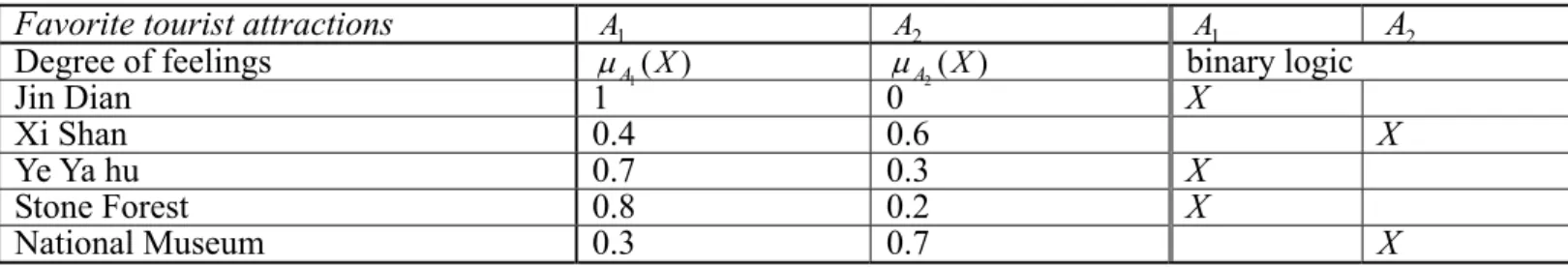
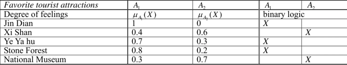
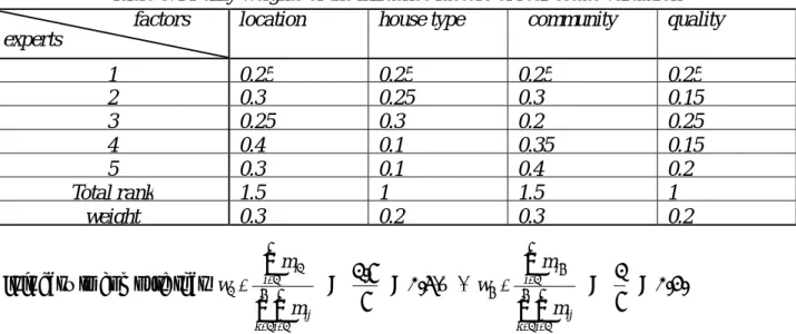
Let U be the universal set (a discussion domain), L={ , , , }L L_{1 2 L} L_k a set of k-linguistic variables on U , and A={A₁,A₂,_L,A_m}and B={B₁,B₂,_L,B_n} be two sets of fuzzy sample drawn from categorical populations with numbers on U. For each sample we assign a linguistic variable L_jand a normalized membership

1 (k 1) ij ij j m m = ∑ = , and let ∑ = = m i ij Aj Ln Fn 1 , ∑ = = n i ij Bj Ln Fn 1 k

j=_{1 L},2, , be the total memberships for each data set.. The following statements are process for testing hypothesis

Testing hypothesis of fuzzy equal for discrete fuzzy mean

Consider a k-cell multinomial vector n={ n₁,n₂,...,n_k}with ∑_{i i}n =n . The Pearson Chi-squared test ( =∑ ∑ − i j ij ij ij e e n 2

χ ) is a well known statistical test for investigating the significance of the differences between observed data arranged in k classes and the theoretically expected frequencies in the k classes. It is clear that the large discrepancies between the observed data and expected cell counts will result in larger values of _χ2

However, a somewhat ambiguous question is whether (quantitative) discrete data can be considered categorical data, for which the traditional_χ2_{-test can be used. For example, suppose a child is asked the following question: “how}

much do you love your sister?” If the responses is a fuzzy number (say, 70% of the time), it is certainly inappropriate to use the traditional _χ2_{-test for the analysis. We will present a χ}2_{-test for fuzzy data as follows:}

Procedures for Testing hypothesis of fuzzy equal for discrete fuzzy mean

1. Hypothesis: Two populations have the same distribution ratio. 2. Statistics： ∑ ∑ ∈ = − = B A i c j _ij ij ij e e Fn , 1 2 2 ([ ] )

χ . ( In order to perform the Chi-square test for fuzzy data, we transfer the decimal fractions of Fn in each cell of fuzzy category into the integer _ij [Fn by counting _ij] 0.5 or higher fractions as 1 and discard the rest.)

3. Decision rule：under significance levelα, ifχ2>χ_α2(k−1),then we reject H₀.

Testing hypothesis of fuzzy index equal for discrete fuzzy mean

Let FX be the fuzzy sample mean ,X f be the defuzzyfication of FX . Under the fuzzy significant level F_δ, and the

corresponding critical value F_δ, we want to test H₀: FX =Fµ, where Fµis the fuzzy mean of the underlying population. Let µ is the defuzzyfication value of Fµ, then the above hypothesis becomesH₀: µ=µ₀.

1 Hypothesis: H₀:F =µ Fµ₀ vs. H₁:F ≠µ Fµ₀.

2. Statistics: find FX from a random sample

{

S_i,i=1,...,n

}

.

3. Decision rule: under the fuzzy significant level F_δ, if X_f −µ₀ ＞δ ,then reject H . ₀

Note: for left side testH ：₀ µ ≤ µ₀ vs. H ：₁ µ>µ₀ under the fuzzy significant level F_δ, ifµ₀-X ＞_f δ , we reject

0

H . The right hand side testing is similar.

Testing hypothesis with continuous fuzzy mean

1 Hypothesis: H ：₀ Fµ = ［a, b] vs. _F H ：₁ F ≠µ _F［a, b].

2. Statistics: find FX =［x ,_l x ] from a random sample _u

{

S_i,i=1,...,n

}

.

3. Decision rule: under the significant level F_δ, find k=δr (where r=b-a), if x_l − ＞k ora x_u − ＞k then reject b H . ₀

4.2 Testing Hypothesis for fuzzy belongs to

Testing of fuzzy belongs to with bounded sample

1 Hypothesis: H ：₀ Fµ∈ ［a, b] vs. _F H ：₁ Fµ∉ ［a, b]. _F

2. Statistics: find FX =［x ,_l x ] from a random sample _u

{

S_i,i=1,...,n

}

.

3. Decision rule: under the significant level F_δ, find k=δr (where r=b-a), ifx ＜a-k or_l x >b+k, _u then reject H . ₀

Testing of fuzzy belongs to with unbounded below sample

1 Hypothesis: H ：₀ Fµ∈ (-_F ∞ , b] vs. H ：₁ Fµ∉ (- ∞ ,b] . _F

2. Statistics: find FX =（∞ ,x ] from a random sample _u

{

S_i,i=1,...,n

}

.

3. Decision rule: under the significant level F_δ, find k=δr (where r is a constant), ifx >b+k, then reject _u H . ₀

Testing of fuzzy belongs to with unbounded above sample

1 Hypothesis: H ：₀ Fµ∈ ［a, ∞ ) vs. _F H ：₁ Fµ∉ ［a, ∞ ) _F

2. Statistics: find FX =［x ,∞） from a random sample _l

{

S_i,i=1,...,n

}

.

3. Decision rule: under the significant level F_δ, find k=δr (where r is a constant), if x ＜a-k, then reject _l H ₀

4. Case Analysis

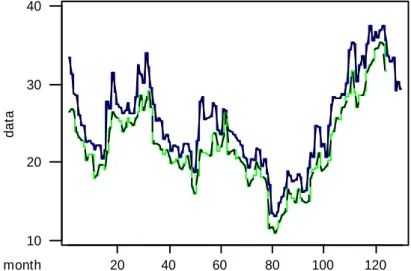
In this section we use a practical case to illustrate the forecasting methods. The interval time series comes from the data that the highest price (b ), the lowest price (_t a ) and the weighted average price (_t m ) of monthly _t

trading values of China Steel stock from January 1995 to October 2005. Then the proposed methods are applied to make the interval forecasting for the last 6 intervals (from May to October). This data comes from the report of monthly trading value of individual stock provided by Taiwan Stock Exchange Corporation. The

chart of the interval time series is shown in Figure 2. 20 40 60 80 100 120 10 20 30 40 month dat a

Figure 1 The chart of the monthly trading values of China Steel stock from 1/1995 to 4/2005.

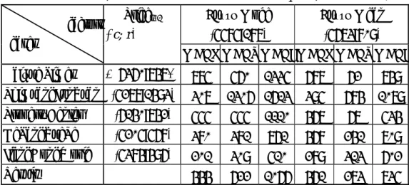
Table 5.1 lists the monthly trading values of China Steel stock from May 2005 to October 2005 and their forecasts by the proposed interval forecasting methods described in Section 3.2. Table 5.2 shows the comparison of the efficiency of the interval forecasting methods.

Table 4.1 The monthly trading values of China Steel stock and their forecasts by the proposed interval forecasting methods for the latter 6 periods from 5/2005 to 10/2005.

Monthly Trading Value of ChinaSteel Stock 5/2005–10/2005

(

c ,t rt

)

/

(

mt,lt,ut

)

Interval Moving Average

(

c ˆˆt,rt

)

Weighted Interval Moving Average

(

c ˆˆt,rt

)

ARIMA of ( c, r) ((2,0,0),(1,0,0))

(

c ˆˆt,rt

)

ARIMA of (m, l, u) ((2,0,0),(0,0,0), (2,0,0))

(

mˆt,lˆt,uˆt

)

(32.08,1.58)/(31.94,1.71,1.44) (31.50,1.35)/(31.51,1.34,1.36) (30.03,1.35)/(31.02,2.43,4.42) (27.70,1.40)/(28.16,0.94,1.86) (29.38,0.98)/(29.33,1.02,0.93) (27.58,1.88)/(27.17,2.28,1.47) (23.57,1.46) (23.52,1.44) (23.48,1.44) (23.44,1.44) (23.42,1.43) (23.41,1.43) (24.29,1.79) (24.17,1.75) (24.11,1.75) (24.09,1.75) (24.06,1.74) (24.06,1.74) (32.60,1.62) (32.03,1.51) (31.60,1.48) (31.23,1.47) (30.89,1.47) (30.58,1.47) (32.59,1.39,1.54) (32.06,1.39,1.60) (31.65,1.39,1.56) (31.29,1.39,1.56) (30.95,1.39,1.55) (30.62,1.39,1.55)

Table 4.2 The comparison of efficiency of the proposed interval forecasting methods for the interval time series of monthly trading values of China Steel stock.

Criteria Interval Moving

Average Weighted Interval Moving Average ARIMA of ( c, r ) ((2,0,0),(1,0,0)) ARIMA of ( m, l, u ) ((2,0,0),(0,0,0),(2,0,0)) MSEP 41.65 33.82 4.48 4.24 MSEL 0.73 0.63 0.70 0.92 MSEI 42.38 34.45 5.18 5.16 MRIE 2.04 1.65 0.57 0.57

From the above analysis result, the forecast results of this interval time series are extremely similar with that of the model (4.3). It shows that the interval time series is nonstationary but steadily increasing or decreasing. So the interval moving average and the weighted interval moving average can only offer the prediction of the interval length. While ARIMA

(

(

p_c,d_c,q_c

) (

, p_r,d_r,q_r

)

)

of

( )

c;r and

(

) (

) (

)

(

pm dm qm pl dl ql pu du qu

)

ARIMA , , ; , , , , , of

(

m ,;l u

)

can perform better forecasting concurrently for the position and the length of intervals. In addition, their mean relative interval errors are fairly small, which shows the overlapping range of the predicted intervals and the actual intervals is larger, so it is concluded that both are excellent forecasting methods. On the other hand, the mean relative interval errors of the interval moving average and the weighted interval moving average are relatively great, which shows that there are few overlapping part of the predicted intervals and the actual intervals, so these two forecasting methods are not suitable for this case.

5. Conclusions

In the progress of the scientific research and analysis, the uncertainty in the statistical numerical data is the crux of the problem that the traditional mathematical model is hard to be established. Manski (1990) has pointed out that the numerical data are over-demanded and over-explained. If we exploit this artificial accuracy to do causal analysis or measurement, it may lead to the deviation of the causal judgment, the misleading of the decision model, or the exaggerated difference between the predicted result and the actual data. This paper proposes to use the interval data to avoid such risks to happen. By means of the interval operations, this paper also discusses the model establishment and forecasting of interval time series. From the research results, it is found that the forecasting of ARIMA interval time series performs more accurate, no matter in the comparisons of the mean squared error of interval or the mean relative interval error, than the traditional forecasting methods such as the moving average and the weighted moving average, etc. Especially for the threshold time series, the forecasting results are much better.

In fact, using interval data to establish model and predict, we can find that the forecasting in each step is carried out by means of intervals, so as to increase the objectiveness of the forecasting results. In the general aspect, the "intervalization" seems to be a very normal phenomenon too. But on the contrary, if the concept of dealing with numerical data does not change and the forecasting method does not make a breakthrough, it often hampers the objectivity of measurements and the possibility of long-term forecasting. If we measure interval time series with the center and the length of intervals, it demonstrates clearly that interval time series has better forecasting ability than the traditional ARIMA method does. However, according to the interval operations and the ARIMA method, it is noteworthy that if we can establish the good model construction process, we can make a superior interval forecasting for the interval time series of stock trading values. For investors, it not only provides a new forecasting method, but also offers more flexible prediction result. Therefore, investors can make more objective judgment under correct information.

Although the approaches proposed in this paper perform interval forecasting effectively, there are some problems still remaining to be solved and some improvement can be done for further research, which are described respectively as follows.

(1) There are so many unpredictable factors on the monthly trading values of stocks, such as trading volumes, exchange rates, interest rates or even the influence of the government policy etc. Consequently, in respect to interval time series proposed in this paper, we only consider the monthly highest price and the monthly lowest price as the range of the monthly trading price caused by all factors. If it needs to make the result more accurate, it can consider finding out the key factors of influencing the interval range.

(2) With regard to interval time series, in order to achieve more accurate result, it needs to make the collected data stationary to make further analysis. But, how to judge if an interval time series is stationary? This paper considers the stationariness of interval location and interval length respectively. Is it possible to find another approach to judge the stationariness of interval time series by other interval operations?

(3) Because the research of interval data forecasting is rare in the past, as generating interval time series data by simulation, we can consider other simulation approaches, such as Bootstrap, Bayesian, Bayesian, etc. The variety of the simulation methods will contribute to the improvement of the forecasting methods. (4) In the analysis and forecasting of interval time series, how to estimate the forecasting accuracy of

interval data is an important issue. There are found four forecasting situations, the forecast interval is too wide, the forecast interval is too narrow, the forecast interval inclines to the right, and the forecast

interval inclines to the left. From the overlapping parts and the nonoverlapping parts of the actual intervals and the forecast intervals, it should be defined a criterion which is more sufficient to show the efficiency of interval forecasting.

References

[1] Wu, B. (1995). Introduction to Time Series Analysis, HwaTai: Taipei.

[2] Montgomery, D. C. and Johnson, L. A. (1976), Forecasting Time Series Analysis, New York:

McGraw-Hill.

[3] Abraham, B. and Ledolter, J. (1983), Statistical Methods for Forecasting. New York: John Wiley.

[4] Chatfield, C. (1989), The Analysis of Time Series (4th ed.), London: Chapman and Hall.

[5] Granger, C.W.J., White, H. and Kamstra, M. (1989), Interval Forecasting: An analysis based upon ARCH-quantile estimators, Journal of Econometrics, 40, 87–96.

[6] Chatfield, C. (1993), Calculating interval forecasts, Journal of Business and Economic Sataiatics, 11,

121–135.

[7] Diebold, F. X. and Mariano, R. S. (1995), Comparing Predictive Accuracy, Journal of Business and Economic Statistics, 13, 253–265.

[8] Christoffersen, P. F. (1998), Evaluating interval forecasts, International Economic Review, 39, 841–862.

[9] Freedaman, D. A. and Peter, S. C. (1984), Bootstrapping a Regression Equation: Some Empirical Results, Journal of the American Statistical Association, 79, 97–106.

[10] Thombs, L. A. and Schucany, W. R. (1990), Bootstrap Prediction Intervals for Autoregression, Journal of the American Statistical Association, 85, 486–492.

[11] McCullough, B. D. (1994), Bootstrapping forecast intervals: An application to AR(p) models, Journal of Forecasting, 13, 51–66.

[12] McCullough, B. D. (1996), Consistent forecast intervals when the forecast-period exogenous variables are stochastic, Journal of Forecasting, 15, 293–304.

[13] Winkler, R.L. (1972), A Decision-Theoretic Approach to Interval Estimation, Journal of the American Statistical Association, 67, 187–191.

[14] Thompson, P. A. and Miller, R. B. (1986), Sampling the future: A Bayesian approach to forecasting from univariate time series models, Journal of Business & Economic Statistics, 4, 427–436.

[15] Barnett, G., Kohn, R. and Sheather, S. (1996), Robust estimation of an autoregressive model using Markov chain Monte Carlo, Journal of Econometrics, 74, 237–254.

[16] Chatfield, C. (1996), Model uncertainty and forecast accuracy, Journal of Forecasting, 15, 495-508.

[17] Faraway, J. and Chatfield, C. (1998), Time-series forecasting with neural networks: A comparative study using the airline data, Applied Statistics, 47, 231–250.

[18] Young, R. C. (1931), The algebra of many-valued quantities, Mathematische Annalen, 104, 260–290,

Also at http://www.cs.utep.edu/interval-comp/young.pdf.

[19] Dwyer, P. S. (1951), Linear Computations. New York: John Wiley and Sons.

[20] Zamowitz, V. and Braun, P. (1993), Twenty-two years of the NBER-ASA Quarterly Economic Outlook surveys. J. H. Stock and M. Watson (eds.), Business Cycles, Indicators and Forecasting, University of

Chicago Press, Chicago.

[21] Granger, C.W.J. (1996), Can we Improving the Perceived Quality of Economic Forecasts? Journal of Applied Econometrics, 11, 455–473.

[22] Wu, B. and Chen, M. (1999). Use fuzzy statistical methods in change periods detection. Applied Mathematics and Computation. 99, 241-254.

[23] Hayes, B. (2003), A Lucid Interval. American Scientist,91,484-488.

[24] Akaike, H. (1969), Fitting autoregressive models for prediction, Annals of the Institute of Statistical Mathematics, 21, 243–247.

[25] Manski, C. (1990), The Use of Intention Data to Predict Behavior: A Best Case Analysis. Journal of the American Statistical Association, 85, 934–940.

[26] Box, G. E. P. and Jenkins, G. M. (1976), Time Series Analysis : Forecasting and control, San Francisco:

Holden-Day.

[27] Introduction to time series analysis. http://www.itl.nist.gov.

國科會補助專題研究計畫成果報告自評表

請就研究內容與原計畫相符程度、達成預期目標情況、研究成果之學術或應用價

值（簡要敘述成果所代表之意義、價值、影響或進一步發展之可能性）

、是否適

合在學術期刊發表或申請專利、主要發現或其他有關價值等，作一綜合評估。

1. 請就研究內容與原計畫相符程度、達成預期目標情況作一綜合評估

9 達成目標

未達成目標（請說明，以 100 字為限）

實驗失敗

因故實驗中斷

2. 研究成果在學術期刊發表或申請專利等情形：

„ 論文：□已發表 □未發表之文稿 □撰寫中 □無

專利：□已獲得 □申請中 □無

技轉：□已技轉 □洽談中 □無

其他：（以 100 字為限）

3. 請依學術成就、技術創新、社會影響等方面，評估研究成果之學術或應用價

值（簡要敘述成果所代表之意義、價值、影響或進一步發展之可能性）（以

500 字為限）

The forecasting of ARIMA interval time series performs more accurate, no matter in the comparisons of the mean squared error of interval or the mean relative interval error, than the traditional forecasting methods such as the moving average and the weighted moving average, etc. Especially for the threshold time series, the forecasting results are more appropriate and realistic in applications.

Using interval data to establish model and predict, we can find that the forecasting in each step is carried out by means of intervals, so as to increase the objectiveness of the forecasting results. In the general aspect, the "intervalization" seems to be a very normal phenomenon too. But on the contrary, if the concept of dealing with numerical data does not change and the forecasting method does not make a breakthrough, it often hampers the objectivity of measurements and the possibility of long-term forecasting. If we measure interval time series with the center and the length of intervals, it demonstrates clearly that interval time series has better forecasting ability than the traditional ARIMA method does.

However, according to the interval operations and the ARIMA method, it is noteworthy that if we can establish the good model construction process, we can make a superior interval forecasting for the interval time series of stock trading values. For investors, it not only provides a new forecasting method, but also offers more flexible prediction result. Therefore, investors can make more objective judgment under correct information. Because the research of interval data forecasting is rare in the past, as generating interval time series data by simulation, we can consider other simulation approaches, such as Bootstrap, Bayesian, Bayesian, etc.

行政院國家科學委員會補助國內專家學者出席國際學術會議報告

2009 年 9 月 16 日 報告人姓名 吳柏林 服務機構及職稱 國立政治大學應用數學系教授 時間 會議 地點 2009/8/2~8/7 泰國清邁 本會核定 補助文號 計畫編號 NSC962416H004014-MY3

會議名稱 Symposium on Econometrics and Forecasting 發表論文題目

Fuzzy Estimation Methods and their Application in Real Estate Evaluation 一.參加會議經過

The International Symposium on Econometrics and Forecasting, 於 2009 年 8 月 2 日至 8

月 7 日在泰國清邁舉行, 由泰國 Chainmai University 與 Thailand Econometrics

Society 主辦,. 來自各國之學者專家約有 40 餘人參加, 包括地主國泰國外,台灣, Japan, USA, Canada, Hongkong, 澳洲, 馬來西亞,等 10 餘國. The conference is held for promoting researches on the Econometrics and soft computing. In recent years, researches on logistics, service, supply chain and knowledge management have become prosperous. In addition, new applications of Mobile business derived from e-Commerce are developing fast and widely. New concepts and theories from above have promoted ubiquitous communication and collaboration. Thanks all participants to attend and present recent results and discuss on management engineering from the perspective of knowledge management and e-Commerce.

2本次大會就以下幾項重點主題進行研討

1. New development in Econometrics 2. Soft computing 3. Intelligent computing 4.knowledge management. 除此之外, 尚有幾個序列的 Workshops 與 Panel discussions 討

論有關 computing Economisc 等. 歐國家如泰國等教授在會中特別提到: Intelligent

Computing 與 Soft Computing 之工程經濟觀點. Mangement challenges in times of global change and uncertainty. 以及一些新觀念如: Perception based reasoning, 區間計算，模糊樣 本分析，知識經濟與創新計算等新看法。

二. 攜回的資料：

1. Symposium on Econometrics and Forecasting 研討會論文集 2.與 Professor Songsak, Professor Sonpond, Professor SAATTakada 等學者討論有關最近著作與研究結果。

三. 建議與其他 目前筆者在政大應數研究所開設人工智慧與時間數列分析與預測課程多年，深感學 術研究發展日新月異、一日千里。國科會能給予補助出國出席國際學術研討會，收穫相 當大。希望將來能多利用課餘時間出國做短期研究，吸收國外新知、及研究方向。回國 後繼續開設模糊時間數列分析與預測課程，指導博、碩士班研究生，籌辦國際學術研討 會，推動國際經濟與管理學術研究工作。並於國際著名學術論文期刊，發表學術論文。 附件四