Identifying the combination of genetic factors that determine susceptibility to cervical cancer

(1)

Identifying the Combination of Genetic Factors That

Determine Susceptibility to Cervical Cancer

Jorng-Tzong Horng, K. C. Hu, Li-Cheng Wu, Hsien-Da Huang, Feng-Mao Lin, S. L. Huang, H. C. Lai, and T. Y. Chu

Abstract—Cervical cancer is common among women all over the world. Although infection with high-risk types of human papillo-mavirus (HPV) has been identified as the primary cause of cer-vical cancer, only some of those infected go on to develop cercer-vical cancer. Obviously, the progression from HPV infection to cancer involves other environmental and host factors. Recent population-based twin and family studies have demonstrated the importance of the hereditary component of cervical cancer, associated with ge-netic susceptibility. Consequently, single-nucleotide polymorphism (SNP) markers and microsatellites should be considered genetic factors for determining what combinations of genetic factors are involved in precancerous changes to cervical cancer. This study employs a Bayesian network and four different decision tree al-gorithms, and compares the performance of these learning algo-rithms. The results of this study raise the possibility of investiga-tions that could identify combinainvestiga-tions of genetic factors, such as SNPs and microsatellites, that influence the risk associated with common complex multifactorial diseases, such as cervical cancer. The web site associated with this study is http://140.115.155.8/Fac-torAnalysis/.

Index Terms—Bayesian network, cervical cancer, decision tree, genetic factors.

I. INTRODUCTION

C

ERVICAL cancer kills more than 1000 women in Taiwan and 200 000 worldwide each year [1], [2]. Epidemiolog-ical studies demonstrate that a positive human papillomavirus (HPV) test is the most significant independent risk factor for the development of both cervical dysplasia and invasive cancer [3]. Compared to HPV status, the relative risk associated with tra-ditional factors such as sexual behavior becomes insignificant [3]. Although researchers have identified HPV as the primary cause of cervical cancer, only some infected individuals actu-ally develop cervical cancer [4], [5]. Other environmental and host factors are involved in the progression of HPV infection to Manuscript received August 7, 2003: revised December 4, 2003. This work was supported in part by the National Science Council, Taiwan, under Contract NSC92-3112-B-008-003.

J.-T. Horng is with the Department of Life Science and the Department of Computer Science and Information Engineering, National Central University, Jhongli City 320, Taiwan, R.O.C. (e-mail: horng@db.csie.ncu.edu.tw).

K. C. Hu, L.-C. Wu, and F.-M. Lin are with the Department of Com-puter Science and Information Engineering, National Central University, Jhongli City 320, Taiwan, R.O.C. (e-mail: kaichih@ db.csie.ncu.edu.tw; richard@db.csie.ncu.edu.tw; meta@db.csie.ncu.edu.tw).

H.- D. Huang is with the Department of Biological Science and Technology and Institute of Bioinformatics, National Chiao-Tung University, Hsin-Chu, Taiwan, R.O.C. (e-mail: damay@db.csie.ncu.edu.tw).

S. L. Huang is with the Department of Life Science, National Central Uni-versity, Jhongli City 320, Taiwan, R.O.C.

H. C. Lai and T. Y. Chu are with Department of Gynecology and Obstetrics, Tri-Service General Hospital, Taipei 114, Taiwan, R.O.C.

Digital Object Identifier 10.1109/TITB.2004.824738

high-grade squamous intraepithelial lesions (HSIL) and cervical cancer [6]. Although most low-grade and many high-grade dys-plastic lesions appear to resolve without intervention, women are still advised to have follow-up examinations and treatments to ensure that the significant subset of women at high risk for de-veloping cancer are treated [7]. Identifying host determinants of viral persistence may help better understand the mechanisms of tolerance, and also may lead to the development of tests permit-ting more focused follow-up of high-risk individuals [7]. Fol-lowing the completion of the human genome project and the exploration of gene polymorphisms, individual susceptibility to cervical cancer can be explored at the genetic level.

The focus of genetics research is on associating sequence variations with inheritable phenotypes. The most common se-quence variation involves SNPs and microsatellites. SNP stands for single-nucleotide polymorphism, which describes a point mutation carried by some individuals within a population. Most SNPs, approximately two out of three, have nucleotide cytosine (C) replaced with thymine (T). The human genome is thought to include over 200 000 SNPs in genes, and probably ten times this number, possibly more, in nongenic DNA [8]. Some research [9] has implicated the proline/argine polymorphism of the codon 72 of the tumor-suppressor gene p53 in the development of cervical cancer, based on the observation that the p53 protein is more ef-ficiently inactivated by the E6 oncoprotein of HPV in p53 argi-nine than by its proline isoform [10]. However, other research presents evidence refuting this relation [11]–[13]. Other SNPs, such as those on genes MCP, IL4, IL10, Smad 2, Smad 4, MMP, and CAV-1, also may be related to cervical cancer [14]–[18].

Microsatellites are also known as short tandem repeats (STR), because a repeated unit comprises only 1 to 6 bps while the complete repeated region spans less than 150 bps. Microsatel-lites have proven useful to geneticists not only because of their value as physical markers in genome mapping, but also be-cause of their applications in linkage analyses in the association with disease susceptibility genes [19]. Microsatellite DNA al-terations are an integral part of neoplastic progression and are valuable clonal markers for detecting human cancers [20]. Cer-vical carcinoma is linked to HPV infection, but microsatellite in-stability could also be involved in cervical tumorigenesis [21]. Research demonstrates that genomic instability occurs during the late stages of the carcinogenesis of cervical cancer, and is associated with the conversion of cervical intraepithelial neo-plasia to an invasive phenotype [22].

Identifying and characterizing the genetic factors deter-mining susceptibility to common complex multifactorial human diseases such as cervical cancer remains statistically and computationally challenging. This study adopts SNPs and 1089-7771/04$20.00 © 2004 IEEE

(2)

60 IEEE TRANSACTIONS ON INFORMATION TECHNOLOGY IN BIOMEDICINE, VOL. 8, NO. 1, MARCH 2004

TABLE I

TYPES OFSNP POLYMORPHISMS IN THEPRESENTDATASET

microsatellites as the genetic factors affecting cervical cancer. The decision tree algorithm [23]–[26] and Bayesian network theory [27] are applied in this work to identify the genetic factors governing susceptibility to cervical cancer.

II. MATERIAL

A retrospective hospital-based case-control study was per-formed. The study cases included 224 patients with normal status, 106 patients with low-grade squamous intraepithelial lesions (LSIL), 152 patients with high-grade squamous in-traepithelial lesions (HSIL), and 238 patients with invasive cervical cancer, all diagnosed and treated at the Tri-Service General Hospital, Taipei, Taiwan, R.O.C. The dataset included 720 records, most with missing values. Each record contained 11 SNP markers, four microsatellites, age, HPV type, and diagnosis. These SNP markers and microsatellites were chosen based on the research in Lai’s work [15]. Table I lists the types of SNP polymorphisms considered in this investigation. The four microsatellites include MMP9, IFNG, IL10G, and IL10R. HPV types are grouped according to their phylogenic similarity [15]. Group 16 includes HPV 16, 31, 33, and 35; group 18 includes HPV 18, 39, 45, 51, 53, 59, 68, 69, MM4, and MM7; and group 58 includes HPV 33, 52, 53, and 58. The values of the diagnosis are 1, 2, 3, or 4, referring to normal status, LSIL, HSIL, and squamous cell carcinomata (SCC), respectively.

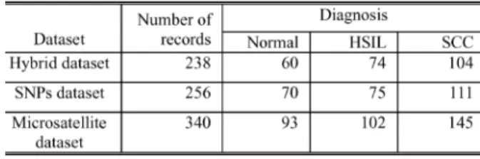
Each record in the hybrid dataset contains various features, including SNP markers, four microsatellites, HPV group, age, and diagnosis. The hybrid dataset comprises two parts. One part, denoted as the SNP’s dataset, consists of 11 SNP markers, HPV group, age, and diagnosis. The other part, denoted as the mi-crosatellite dataset, consists of four mimi-crosatellites, HPV group, age, and diagnosis. Table II lists the diagnosis distribution for each dataset after removing records with missing values. The SNP dataset contains 256 records. Seventy of these records are diagnosed as normal; 75 are diagnosed as high squamous in-traepithelial lesions, and 111 are diagnosed as squamous cell carcinomata. The hybrid dataset includes both microsatellite and SNP’s data, but records with missing values in any SNP markers or microsatellites in the dataset are excluded. Thus, the

TABLE II

AMOUNT OFDATA ANDDIAGNOSISDISTRIBUTION OFEACHDATASETAFTER

REMOVINGRECORDSWITHMISSINGVALUES. THEHYBRIDDATASETHAS

MISSINGVALUES AND SOITCONTAINSFEWERRECORDSTHAN THE

OTHERTWODATASETS

hybrid dataset includes only 238 records, which is less than the 256 records in the SNP dataset and the 340 records in the mi-crosatellite dataset. Since most of the data with the diagnosis of low squamous intraepithelial lesions (LSIL) have missing values, Table II does not display data with LSIL diagnosis, and such data is not used in this investigation.

III. METHODS

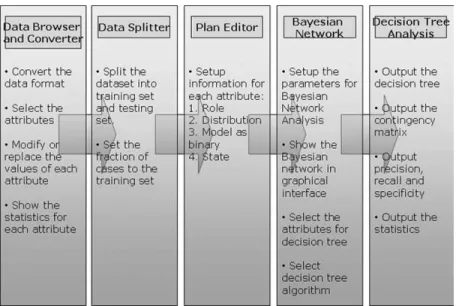
This study implements a web-based system that predicts com-binations of sSNPs and microsatellites as possible cofactors of cervical cancer. Fig. 1 gives the system flow of the method de-veloped here for identifying the combination of genetic factors that determine susceptibility to cervical cancer.

First, the Data Browser and Converter allows users to ignore the quotes, delete all spaces in the dataset, replace all keywords “or” with commas, and ignore the rows with missing values. The system can automatically detect data that needs to be converted. If the converted data file is detected, users can ignore the con-version process. The statistics page in the data browser displays the statistics of each variable, and users can specify that each variable can be treated as a continuous variable or merged with other variables. The variable can have many different values, and most values that appear once are automatically pre-assigned as continuous variables.

The Data Splitter is used to divide the dataset into training and testing datasets. The Bayesian network model and decision tree can be established by learning from the training dataset and testing using the testing dataset. Users can specify either the fraction or number of cases to be assigned to the training set. The default fraction of splitting is 70% for training and 30% for testing.

Third, the Plan Editor establishes a plan file that contains the information required for creating the Bayesian network. Par-ticularly, the role of each variable should be specified in this step. Each variable can be an input variable (used to predict other variables), an output variable (predicted by other ables), an input–output variable (both predicted by other vari-ables and used to predict other varivari-ables), or ignored (not used). A variable within the network can be chosen as “input” variable if the content of the variable only affects other variables and will not be affected by other variables. For example, the vari-able “age” is defined as an input varivari-able. Similarly, a varivari-able can be selected as an “output” variable if it is assumed to be af-fected by other variables; for example, the variable “diagnosis” is an output variable. Most variables in the network examined

(3)

Fig. 1. System flow for identifying susceptible genotypes for cervical cancer. here are defined as input–output variables, meaning they might affect other variables and also might be affected by other vari-ables.

Next, Bayesian belief network analysis is performed. The Bayesian belief network specifies the joint conditional prob-ability distributions between variables [27]. The Bayesian be-lief network allows class conditional independencies to be de-fined between subsets of variables, and also provides graph-ical models of causal relationships, on which learning can be performed. These networks are also known as belief networks, Bayesian networks, and probabilistic networks. Each variable in the network is treated as a node. Each edge in the Bayesian belief network represents the joint conditional probability dis-tributions between variables. An edge connecting two nodes means that stronger causal relationships exist between these two variables than between variables without such edge connection. Restated, two nodes without an edge connection demonstrate the existence of independence between these two variables. The Bayesian belief network might contain more than one output variable. Inference algorithms for learning can be applied to the Bayesian belief network which contains multiple output vari-ables. Rather than returning a single class label variable, the Bayesian inference algorithm can return a probability distribu-tion for the class label variables. For the present dataset, the di-agnosis is selected as the only output variable, and the infer-ence algorithm is not used in the present method. The level of complexity of the Bayesian belief network and the dataset for the network should be specified before showing the network. The Bayesian belief network complexity level is the threshold for showing the network and avoiding displaying a fully con-nected graph. The complexity level is represented as a value be-tween zero and one. The default complexity level value is one, which indicates a most simplified network. The input data for thee Bayesian belief network could be the whole dataset, the training dataset, or the testing dataset. Users can select variables with connected edges to build decision trees rather then using all variables.

The final process is to create a decision tree. A decision tree is a flowchart with a structure shaped like a tree, in which each

internal node denotes a test on a variable, each branch repre-sents a test outcome, and leaf nodes represent classes or class distributions. This study applies four decision tree algorithms, namely, the J48 [23], PART [26], ID3 [24], and PRISM [25] al-gorithms. ID3 is a divide-and-conquer decision tree algorithm [24]. J48 and ID3 are the practical learning schemes used in the well-known C4.5 decision tree program [23], [24]. PRISM is a covering algorithm for rule generation and is a variation of ID3 algorithm [25]. The variables used to run decision trees can be specified, and users can use all variables in the dataset or can specify the variables with edge connected with output node in the Bayesian network. Expert knowledge, such as halpotype or pathway relation, can be specified by selecting variables indi-vidually. The option “use reduced error pruning” is the default value in the J48 and PART decision trees. Moreover, the option “use reduced error pruning” can shrink a J4.8 decision tree or reduce the number of rules produced by PART, and moreover has the side effect of reducing run time because the complexity depends on the number of rules generated. However, “reduced error pruning” often reduces the accuracy of the resulting de-cision trees and rules, because it reduces the amount of data that can be used for training. This disadvantage vanishes given sufficiently large datasets. The default confidence threshold for pruning of the PART algorithm is set to 0.25, and the minimum number of instances per leaf is set to two. Increasing the confi-dence threshold for pruning may also reduce the accuracy of the result and may result in a smaller tree. The minimum number of instances per leaf is used to avoid creating a huge tree with only one instance per leaf.

IV. RESULTS

This study implemented a web-based system for predicting combinations of SNPs and microsatellites as genetic factors for cervical cancer. System performance was compared under various learning conditions, using different decision tree algorithms and different parameters for constructing decision trees. The batched processing mode is useful for making comparisons, because several decision trees can be constructed

(4)

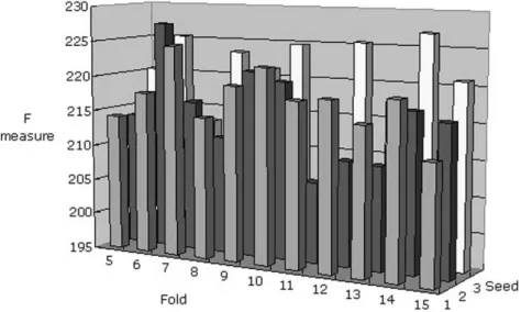
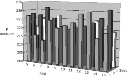
Fig. 2. Performance comparison for the hybrid dataset using the PART algorithm. Sixfold cross-validation and two seeds were adopted as the appropriate comparison conditions because this parameter setting maximizes the F measure.

TABLE III

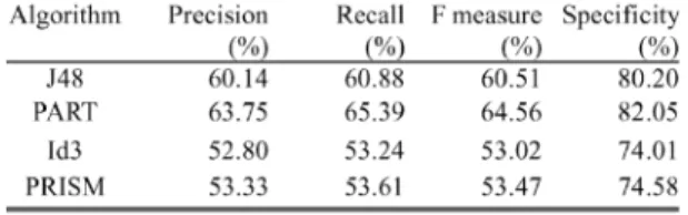
PRECISION, RECALL, F MEASURE,ANDSPECIFICITY FOR THEHYBRIDDATASET

USINGDIFFERENTDECISIONTREEALGORITHMS. THEPART ALGORITHM

OUTPERFORMED THEOTHERALGORITHMS

simultaneously. Batch processing was adopted to achieve this goal. After completing the batch processing, the system automatically selects the optimal model from several decision tree models, according to the F measure derived from the contingency matrix [28]. Table III lists the elements of the contingency matrix for a given diagnosis C, which may be normal status, HSIL, or SCC. For example, of diagnosis SCC indicates the number of records with diagnosis of SCC and correctly predicted as being SCC. of diagnosis SCC represents the number of records with diagnosis of SCC and incorrectly predicted as not being SCC (HSIL or normal). Some definitions are used for performance measurement. Precision [29], recall [29], and specificity [30] are defined by

(1) (2) (3) Precision and recall are widely used in various information systems [29]. Recall is also called sensitivity. Sensitivity and specificity are frequently used in clinical analysis applications [30]. Dissatisfaction with previous methods of measuring effec-tiveness using a pair of numbers (such as precision and recall) that may co-vary in a loosely specified way has stimulated at-tempts to devise composite measures. Such composite measures are based on the contingency matrix, but combine different parts

TABLE IV

Fig. 3. PART decision tree result for the hybrid dataset.

of this matrix into a single numeric measure, such as the F mea-sure [28]. The F meamea-sure is derived from the contingency matrix, and defined as

(4) where and represent precision and recall, respectively.

The system learns and outputs the decision tree model during training. The model is evaluated with data which were not used in training. This study follows an approach called -fold cross-validation [31]. First, the total dataset is split into equal parts. Next, training/test cycles are performed. For each cycle of , part is used for testing and the other parts are used for training. The final assessment of the decision tree is based on the average of the scores obtained during all of these cycles. As described previously, the F measure is obtained as the final assessment score. In this approach, each record in the dataset is used to train cycles and test one cycle. Sometimes, the cross-validation is repeated several times, each time with the data reshuffled, and consequently, the random number seed can be set in these algorithms.

Individual algorithm performances were compared under var-ious conditions to choose the most appropriate for applying all

(5)

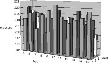
Fig. 4. Comparison of the performance for the SNP’s dataset using the J48 algorithm. Tenfold cross-validation and one seed were selected as the appropriate conditions for the SNP’s dataset.

TABLE V

learning algorithms. Only 239 records in the hybrid dataset had no missing values, limiting the learning conditions to a small and reasonable value range. Thus, the range of fold number in cross-validation is constrained between 5 and 15, and the seed range is constrained between one and three. This study chooses the option “use reduced error pruning” in J48 and the PART decision tree, and did not choose other optimization options while comparing algorithms. Every algorithm is built with a ferent number of folds in cross-validation and also with a dif-ferent number of seeds. Moreover, the F measure is calculated for every algorithm. Table IV compares the performance of the hybrid dataset. The percentages of precision, recall, specificity, and F measure of the four algorithms are compared. Table IV reveals that the PART algorithm outperformed the other algo-rithms. Consequently, the PART decision tree algorithm was ap-plied to a hybrid dataset. Since every record in a cross-valida-tion cycle will be in the test set once, the F measure of every test can be summed to produce a single value. Different numbers of folds in cross-validation and different numbers of seeds are also compared using the summed value of the F measure in Fig. 2. Sixfold cross-validation and two seeds are adopted as the appro-priate conditions based on the F measure. Fig. 3 illustrates the PART decision tree in our result. In the tree structure, a colon introduces the class label that has been assigned to a particular leaf, the label of which is followed by the number of instances of records that reach the leaf, expressed as a decimal number. The decision tree in Fig. 3 involves four variables, namely, age, HPV, and two microsatellites, i.e., IL10R and IFNG.The deci-sion tree clearly indicates that, if the values of both alleles of

Fig. 5. J48 decision tree result for the SNP’s dataset.

Fig. 6. Bayesian network for the SNP’s dataset. The HPV_group is directly connected to diagnosis.

IL10R are 109, the diagnosis is SCC. Meanwhile, if the patients are not infected with HPV, then the diagnosis will be normal. This result also reveals that when the values of the two alleles

(6)

Fig. 7. Performance comparison for the microsatellite dataset. Thirteenfold cross validation and one seed were chosen as the appropriate parameters.

of IL10R are both 109, the diagnosis of cervical cancer will be HSILs if the patient is aged below 39 and the values of the two alleles of IFNG are 117 and 121.

The same analytical procedure is applied to determine the ap-propriate conditions and learning scheme using the SNP dataset. Table V compares the performance of the four algorithms ap-plied to the SNP’s dataset. Table V shows that the J48 algo-rithm outperformed the others. Similarly, Fig. 4 shows the per-formance of different folds and seeds. Tenfold and one seed are selected as parameters based on the F measure. Fig. 5 shows the decision tree results for the SNP’s dataset using the J48 deci-sion tree algorithm. Fig. 5 verifies that HPV is the central cause of cervical cancer. HPV dominates the root of the decision tree, which demonstrates that HPV is a major factor in the decision tree. The decision tree includes five SNPs, namely, MMP1_G-1607G, IL4RA_C-3223T, MCP1_G-2518A, IL12B_A+1188C, and P53_R72P. If the patients are not infected with HPV, then the diagnosis in the decision tree is normal. Meanwhile, if the type of HPV infection is 18 or 58, then the diagnosis in the de-cision tree is SCC. Furthermore, if the HPV type is 16, then various combinations of the five SNPs in the decision tree can predict the diagnosis of cervical cancer. Fig. 6 illustrates the Bayesian network of the SNP’s dataset. The network reveals that MMP1_G-1607G, HPV, and IL4RA_C-3223T directly sup-port the diagnosis of cervical cancer. The Bayesian network and decision tree thus show that MMP1_G-1607G, HPV, and IL4RA_C-3223T are direct inducing variables in diagnosing cervical cancer.

Finally, the microsatellite dataset was analyzed. Table VI compares the performance of different algorithm on mi-crosatellite dataset. Table VI shows that the PART algorithm outperforms other algorithms on microsatellite dataset. Thir-teenfold and one seed are chosen as the appropriate parameters for testing (see Fig. 7 ). Fig. 8 presents the decision tree results obtained using the microsatellite dataset. Notably, HPV also dominates the decision tree in microsatellite dataset in Fig. 8. The decision tree in Fig. 8 contained two microsatellites, IFNG and IL10G. Table VII shows the contingency matrix of the PART decision tree algorithm using thirteenfold and one seed cross-validation on a microsatellite dataset. The contingency

Fig. 8. PART decision tree result for the microsatellite dataset.

Fig. 9. Bayesian network for the microsatellite dataset.

matrix shows that the decision tree performs better on records with normal diagnosis and SCC than on records with diagnosis of HSIL. Only 45 HSILs out of 102 are predicted correctly. Moreover, 73 cases are correctly predicted as having normal status from among 93 diagnosis normal status records and 98 cases of SCC are correctly predicted from among 145 diagnosis SCC. Fig. 9 shows the Bayesian network of the microsatellite dataset. The MMP9 does not have any edge connections, meaning MMP9 is more independent of diagnosis than other variables. The Bayesian network confirms the differences between the works of Shimajiri and Peters on MMP9 [32], [33]. The Bayesian network reveals that IFNG, HPV, and IL10G indirectly determine the diagnosis.

V. DISCUSSION

The idea that epistasis or gene–gene interaction is impor-tant in human biology is not new [34]. In fact, Wright [35] emphasized that the relationship between genes and biological endpoints depends on dynamic interactive networks of genes and environmental factors [34]. Gibson [36] pointed out that

(7)

TABLE VI

PRECISION, RECALL, F MEASURE,ANDSPECIFICITY FOR THEMICROSATELLITE

DATASET. THEPART ALGORITHMOUTPERFORMED THEOTHERALGORITHMS

TABLE VII

CONTINGENCYMATRIX FOR THEMICROSATELLITEDATASET. THENUMBER IN THEDIAGONALENTRYREPRESENTS THENUMBER OFCORRECTLYPREDICTED

RECORDS. THECONTINGENCYMATRIXISACHIEVED BY THEDECISION

TREEUSING THEPART ALGORITHMWITHTHIRTEENFOLD ANDONE

SEED ASPARAMETERS

gene–gene and gene–environment interactions must be ubiq-uitous given the complex intermolecular interactions required to regulate gene expression and the hierarchical complexity of metabolic networks [34].

This study analyzed a dataset provided by Tri-Service Gen-eral Hospital by applying four decision tree algorithms and the Bayesian network theory to identify the combination of genetic factors determining susceptibility to cervical cancer. The dataset included 720 records, each with 18 variables, including 11 SNPs, four microsatellites, age, HPV, and diagnosis. The hybrid dataset contained 238 records after removing those with missing values. The performance of various decision tree algorithms using different parameters is compared by considering the F measure. The PART decision tree algorithm and sixfold cross-validation were used to analyze the hybrid dataset. The decision tree included two microsatellites, i.e., IL10R and IFNG. These two microsatellites also appeared in the decision tree derived from the microsatellite dataset, and were used to predict precancerous or cancer states.

The top performing J48 algorithm was applied to the SNP’s dataset. Tenfold cross-validation was used during cross-validation. Five SNP markers appeared in the deci-sion tree of the SNP’s dataset, namely: MMP1_G-1607GG, IL4RA_C-3223T, MCP1_G-2518A, IL12B_A+1188C, and P53_R72P. The Bayesian network of the SNP’s dataset also showed that MMP1_G-1607G, HPV, and IL4RA_C-3223T directly affect the diagnosis of cervical cancer. IFNG, IL10R, MMP1_G-1607G, and IL4RA_C-3223T thus are identified as the genetic cofactors of cervical cancer.

Identifying and characterizing genetic factors determining susceptibility to common complex multifactorial human diseases remains a statistically and computationally chal-lenging task. This study applied the decision tree algorithm and Bayesian network theory to data to identify the genetic factors governing susceptibility to cervical cancer. From the results presented in this study, the phase of cervical cancer can be predicted through the decision tree of the genetic factors,

i.e., IFNG, IL10R, MMP1_G-1607GG, and IL4RA_C-3223T, although the total number of records in the dataset remains insufficient for further analysis. In conclusion, the analytical results of this study can open the door to identifying the com-binations of genetic factors, such as SNPs and microsatellites, which interact in a nonadditive or nonlinear manner to influ-ence the risk associated with common complex multifactorial diseases.

REFERENCES

[1] J. M. Walboomers, M. V. Jacobs, M. M. Manos, F. X. Bosch, J. A. Kummer, K. V. Shah, P. J. Snijders, J. Peto, C. J. Meijer, and N. Munoz, “Human papillomavirus is a necessary cause of invasive cervical cancer worldwide,” J Pathol., vol. 189, pp. 12–29, 1999.

[2] P. D. Wang and R. S. Lin, “Age-period-cohort analysis of cervical cancer mortality in Taiwan, 1974–1992,” Acta Obstet. Gynecol. Scand., vol. 76, pp. 697–702, 1997.

[3] D. D. Davey and R. J. Zarbo, “Human papillomavirus testing—Are you ready for a new era in cervical cancer screening?,” Arch. Pathol. Lab.

Med., vol. 127, pp. 927–929, 2003.

[4] F. X. Bosch, A. Lorincz, N. Munoz, C. J. Meijer, and K. V. Shah, “The causal relation between human papillomavirus and cervical cancer,” J.

Clin. Pathol., vol. 55, pp. 244–65, 2002.

[5] H. zur Hausen, “Papillomaviruses causing cancer: Evasion from host-cell control in early events in carcinogenesis,” J Nat. Cancer Inst., vol. 92, pp. 690–698, 2000.

[6] F. P. Perera, “Environment and cancer: Who are susceptible?,” Science, vol. 278, pp. 1068–73, 1997.

[7] E. S. Calhoun, R. M. McGovern, C. A. Janney, J. R. Cerhan, S. J. Iturria, D. I. Smith, B. S. Gostout, and D. H. Persing, “Host genetic polymor-phism analysis in cervical cancer,” Clin. Chem., vol. 48, pp. 1218–1224, 2002.

[8] F. S. Collins, M. S. Guyer, and A. Charkravarti, “Variations on a theme: Cataloging human DNA sequence variation,” Science, vol. 278, pp. 1580–1, 1997.

[9] A. Storey, M. Thomas, A. Kalita, C. Harwood, D. Gardiol, F. Mantovani, J. Breuer, I. M. Leigh, G. Matlashewski, and L. Banks, “Role of a p53 polymorphism in the development of human papillomavirus-associated cancer,” Nature, vol. 393, pp. 229–34, 1998.

[10] J. M. Ojeda, S. Ampuero, P. Rojas, R. Prado, J. E. Allende, S. A. Barton, R. Chakraborty, and F. Rothhammer, “PG53 codon 72 polymorphism and risk of cervical cancer,” Biol. Res., vol. 36, pp. 279–283, 2003. [11] A. M. Josefsson, P. K. Magnusson, N. Ylitalo, P. Quarforth-Tubbin, J.

Ponten, H. O. Adami, and U. B. Gyllensten, “P53 polymorphism and risk of cervical cancer,” Nature, vol. 396, p. 531; author’s reply p. 532, 1998.

[12] E. K. Malcolm, G. B. Baber, J. C. Boyd, and M. H. Stoler, “Polymor-phism at codon 72 of p53 is not associated with cervical cancer risk,”

Mod. Pathol., vol. 13, pp. 373–8, 2000.

[13] M. C. Abba, L. M. Villaverde, M. A. Gomez, F. N. Dulout, M. R. Laguens, and C. D. Golijow, “The p53 codon 72 genotypes in HPV infection and cervical disease,” Eur. J. Obstet. Gynecol. Reprod. Biol., vol. 109, pp. 63–6, 2003.

[14] S. Hazelbag, G. J. Fleuren, J. J. Baelde, E. Schuuring, G. G. Kenter, and A. Gorter, “Cytokine profile of cervical cancer cells,” Gynecol. Oncol., vol. 83, pp. 235–43, 2001.

[15] H. C. Lai, C. A. Sun, M. H. Yu, H. J. Chen, H. S. Liu, and T. Y. Chu, “Favorable clinical outcome of cervical cancers infected with human papilloma virus type 58 and related types,” Int. J. Cancer, vol. 84, pp. 553–7, 1999.

[16] A. Mitra, J. Chakrabarti, N. Chattopadhyay, and A. Chatterjee, “Mem-brane-associated MMP-2 in human cervical cancer,” J. Environ. Pathol.

Toxicol. Oncol., vol. 22, pp. 93–100, 2003.

[17] T. F. Chan, T. H. Su, K. T. Yeh, J. Y. Chang, T. H. Lin, J. C. Chen, S. S. Yuang, and J. G. Chang, “Mutational, epigenetic and expressional analyzes of caveolin-1 gene in cervical cancers,” Int. J. Oncol., vol. 23, pp. 599–604, 2003.

[18] T. T. Maliekal, M. L. Antony, A. Nair, R. Paulmurugan, and D. Karuna-garan, “Loss of expression, and mutations of Smad 2 and Smad 4 in human cervical cancer,” Oncogene, vol. 22, pp. 4889–97, 2003. [19] K. G. Ardlie, L. Kruglyak, and M. Seielstad, “Patterns of linkage

dise-quilibrium in the human genome,” Nat. Rev. Genet., vol. 3, pp. 299–309, 2002.

(8)

[20] H. Nawroz, W. Koch, P. Anker, M. Stroun, and D. Sidransky, “Mi-crosatellite alterations in serum DNA of head and neck cancer patients,”

Nat. Med., vol. 2, pp. 1035–1037, 1996.

[21] D. French, C. Cermele, A. Vecchione, and M. Cenci, “HPV infection and microsatellite instability in squamous lesions of the uterine cervix,”

Anticancer Res., vol. 20, pp. 3417–21, 2000.

[22] M. Nishimura, H. Furumoto, T. Kato, M. Kamada, and T. Aono, “Mi-crosatellite instability is a late event in the carcinogenesis of uterine cer-vical cancer,” Gynecol. Oncol., vol. 79, pp. 201–206, 2000.

[23] J. R. Quinlan, C4.5: Programs for Machine Learning. San Mateo, CA: Morgan Kaufman, 1993.

[24] , “Induction of decision trees,” Mach. Learn., vol. 1, pp. 81–106, 1986.

[25] J. Cendrowska, “PRISM: An algorithm for inducing modular rules,” Int.

J. Man-Mach. Studies, vol. 27, pp. 349–370, 1987.

[26] E. Frank and I. H. Witten, “Generating accurate rule sets without global optimization,” presented at the 15th International Conference on Ma-chine Learning, 1998.

[27] F. Jensen, An Introduction to Bayesian Networks. New York: Springer-Verlag, 1996.

[28] V. Hatzivassiloglou, P. A. Duboue, and A. Rzhetsky, “Disambiguating proteins, genes, and RNA in text: A machine learning approach,”

Bioin-formatics, vol. 17, pp. S97–106, 2001.

[29] C. J. v. Rijsbergen, Information Retrieval. London, U.K.: Butter-worths, 1979.

[30] A. R. Feinstein, “Clinical biostatistics. XXXIX. The haze of Bayes, the aerial palaces of decision analysis, and the computerized Ouija board,”

Clin. Pharmacol. Ther., vol. 21, pp. 482–96, 1977.

[31] T. Mitchell, Machine Learning. NewYork: McGraw-Hill, 1997. [32] D. G. Peters, A. Kassam, P. L. St Jean, H. Yonas, and R. E. Ferrell,

“Functional polymorphism in the matrix metalloproteinase-9 promoter as a potential risk factor for intracranial aneurysm,” Stroke, vol. 30, pp. 2612–2616, 1999.

[33] S. Shimajiri, N. Arima, A. Tanimoto, Y. Murata, T. Hamada, K. Y. Wang, and Y. Sasaguri, “Shortened microsatellite d(CA)21 sequence down-reg-ulates promoter activity of matrix metalloproteinase 9 gene,” FEBS Lett., vol. 455, pp. 70–4, 1999.

[34] J. H. Moore and L. W. Hahn, “A cellular automata approach to detecting interactions among single-nucleotide polymorphisms in complex multi-factorial diseases,” in Pac. Symp. Biocomputation, 2002, pp. 53–64. [35] S. Wright, “Evolution in Mendelian populations. 1931,” Bull. Math.

Biol., vol. 52, pp. 241–95, 1931.

[36] G. Gibson, “Epistasis and pleiotropy as natural properties of transcrip-tional regulation,” Theory Popular Biol., vol. 49, pp. 58–89, 1996.

Jorng-Tzong Horng was born in Nantou, Taiwan, R.O.C., on April 10, 1960. He received the Ph.D. degree in computer science and information engi-neering from National Taiwan University, Taipei, R.O.C., in April 1993.

In 1993, he joined the Department of Computer Science and Information Engineering, National Cen-tral University, Jungli, Taiwan, R.O.C., where he be-came Professor in 2002. His current research interests include database systems, data mining, genetic algo-rithms, and bioinformatics.

K. C. Hu is with the Department of Computer Science and Information Engi-neering, National Central University, Jhongli City, Taiwan, R.O.C.

Li-Cheng Wu was born in Taipei, Taiwan, R.O.C., in 1973. He received the Master degree in computer science and information engineering from National Central University, Jhongli City, Taiwan, R.O.C., in 1997.

He is now working toward the Ph.D. degree in computer science and infor-mation engineering, National Central University. His current research interest is bioinformatics and database systems.

Hsien-Da Huang was born in Taoyuan, Taiwan, R.O.C., in 1975. He received the Ph.D. degree in computer science and information engineering in National Central University, Jhongli City, Taiwan, R.O.C., in June, 2003.

In 2003, he join the Department of Biological Science and Technology and Institute of Bioinformatics, National Chiao-Tung University, Hsin-Chu, Taiwan, R.O.C. His current research interest is bioinformatics, database systems, and data mining.

Feng-Mao Lin was born in I-Lan, Taiwan, R.O.C., in 1976. He received Master degree in computer science and information engineering from National Central University, Jhongli City, in 2000.

He is now working toward the Ph.D. degree in computer science and infor-mation engineering at National Central University. His current research interest is bioinformatics and database systems.

S. L. Huang is with the Department of Life Science, National Central Univer-sity, Jhongli City 320, Taiwan, R.O.C.

H. C. Lai is with Department of Gynecology and Obstetrics, Tri-Service Gen-eral Hospital, Taipei 114, Taiwan, R.O.C.

T. Y. Chu is with Department of Gynecology and Obstetrics, Tri-Service Gen-eral Hospital, Taipei 114, Taiwan, R.O.C.