Road-sign detection and tracking

Road-Sign Detection and Tracking

Chiung-Yao Fang, Associate Member, IEEE, Sei-Wang Chen, Senior Member, IEEE, and

Chiou-Shann Fuh, Member, IEEE

Abstract—In a visual driver-assistance system, road-sign

detec-tion and tracking is one of the major tasks. This study describes an approach to detecting and tracking road signs appearing in com-plex traffic scenes. In the detection phase, two neural networks are developed to extract color and shape features of traffic signs from the input scenes images. Traffic signs are then located in the images based on the extracted features. This process is primarily conceptu-alized in terms of fuzzy-set discipline. In the tracking phase, traffic signs located in the previous phase are tracked through image se-quences using a Kalman filter. The experimental results demon-strate that the proposed method performs well in both detecting and tracking road signs present in complex scenes and in various weather and illumination conditions.

Index Terms—Fuzzy integration, hue, saturation, and intensity

(HSI) color model, Kalman filter, neural networks, road-sign de-tection and tracking.

I. INTRODUCTION

R

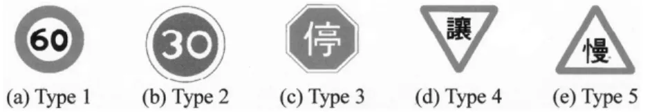
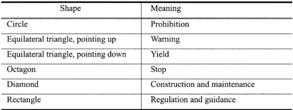
OAD SIGNS are used to regulate traffic, warn drivers, and provide useful information to help make driving safe and convenient. In order to make clear which of these different kinds of information is being provided by any particular sign, several very different basic design styles are used for the signs. These differences are based on unique shapes and colors. Tables I and II illustrate the meanings of various colors and shapes for signs used in Taiwan. While the design and use of road signs has been long established, they do not provide a perfect solution to making driving safe, in part because of the fact that drivers are only human. For example, many accidents have been caused by the failure of a driver to notice a stop sign, either due to a lack of paying attention at a critical moment or due to adverse conditions that impede visibility. At night, drivers are easily dis-tracted or blinded by the headlights of oncoming vehicles. In bad weather (e.g., rain, snow, and fog) road signs are less likely than normal to attract a driver’s attention. All these situations make driving more difficult and can, therefore, lead to more traffic ac-cidents. Computer vision systems are increasingly being used to aid or replace humans in the performance of many tasks re-quiring the ability to see. It is the purpose of this paper to de-scribe such a computer vision system that could be used to notify a human driver to the presence and nature of road signs.

Manuscript received August 2000; revised August 2002. This work was supported by the National Science Council, R.O.C., under Contract NSC-89–2218E-003–001.

C.-Y. Fang is with the Department of Information and Computer Educa-tion, National Taiwan Normal University, Taipei, Taiwan, R.O.C. (e-mail: violet@ice.ntnu.edu.tw).

S.-W. Chen and C.-S. Fuh are with the Department of Computer Science and Information Engineering, National Taiwan Normal University, Taipei, Taiwan, R.O.C.

Digital Object Identifier 10.1109/TVT.2003.810999

In experiments, traffic-scene images were taken in all condi-tions, such as sunny, shady, rainy, cloudy, and windy, as well as all locations, including freeways, expressways, highways, boulevards, streets, and country roads. These factors involve considerably varied lighting conditions and backgrounds. While road signs are comprised of particular colors, the various out-door environments affect the perceived colors of road signs. In addition, moving objects, such as trucks, cars, motorcycles, bi-cycles, and pedestrians, may partially occlude road signs and, therefore, transiently modify the visible shapes of road signs. Moreover, complex backgrounds, e.g., miscellaneous buildings and shop signs, also increase the difficulty of automatically de-tecting road signs. For these reasons, the reliable detection of road signs from such varied scenes becomes rather challenging. Recently, many techniques have been developed to detect road signs [1]–[8]. Most deal with single images with simple backgrounds [9]–[13]. Lalonde and Li [12] reported a color-in-dexing approach to identifying road signs. All models of road signs were first described in terms of color histograms. Iden-tifying a road sign extracted from an image was accomplished by simply comparing its color histogram with those prestored in a database. However, their method failed to account for the structural evidence of road signs. Escalera and Moreno [9] com-bined colors and shapes to detect road signs. First, they used color thresholding to segment the input image. They then ex-tracted special color regions, such as red and blue, from the image. Second, specific angle corners, including 60 and 90 , were used to convolve with these special color regions. Finally, to examine which corners constituted a fixed shape road sign, the shapes of road signs were used. Unfortunately, the number of corners in an image grows rapidly with increasingly complex traffic scenes and this, in term, greatly increases the computa-tional load on the system.

Piccioli et al. [14] also incorporated both color and edge information to detect road signs from a single image. They claimed that to improve the performance, their technique could be applied to temporal image sequences. We agree with their conclusion. In fact, the detection of road signs using only a single image has three problems: 1) to reduce the search space and time, the positions and sizes of road signs cannot be predicted; 2) it is difficult to correctly detect a road sign when temporary occlusion occurs; and 3) the correctness of road signs is hard to verify. By using a video sequence, we preserve information from the preceding images, such as the number of the road signs and their predicted sizes and positions. This information increases the speed and accuracy of road-sign detection in subsequent images. Moreover, information sup-plied by later images is used to assist in verifying the correct detection of road signs, so that detected and tracked objects 0018-9545/03$17.00 © 2003 IEEE

TABLE I

STANDARDROAD-SIGNBACKGROUNDCOLORS ANDTHEIRMEANINGS INTAIWAN

TABLE II

STANDARDROAD-SIGNSHAPES ANDTHEIRMEANINGS INTAIWAN

that are not road signs can be eliminated as soon as possible and, thus, reduce the burden on the processor. Thus, we believe the video sequence provides more valuable information for road-sign detection than does a single image.

Aoyagi and Asakura [15] used genetic algorithms to detect road signs from gray-level video images. They first transformed parameters (position, size, etc.) of road signs into 17-bit genes. Initial seed genes in the original generation were automatically provided and then crossover and mutation operators were em-ployed to generate next-generation genes from the seeds. A fit-ness function was utilized for measuring the quality of all genes in one generation; then, by an elite preservation strategy, 32 genes were selected as seed genes. In their experiments, after 150 generations, the process of evolution is complete. That is, the high-fitness genes were then assumed to represent road signs in the image. Unfortunately, their method did not guarantee that a maximum fitness gene always represents a road sign. In ad-dition, only circular road signs within scene images could be detected and no tracking technique was used to improve the per-formance.

In this study, color video sequences are employed to detect the road signs in complex traffic scenes. A tracking technique, the Kalman filter, is used to reduce the search time for road-sign detection. The outline of our road-road-sign detection system is presented in Section II. Section III addresses the methods of detecting color and shape features. In Section IV, a process characterized by fuzzy-set discipline is introduced to integrate information derived from the incoming video. Section V dis-cusses our use of the Kalman filter. Section VI includes a simple

method to verify the candidates for road signs. Section VII demonstrates the experimental results with real images and Section VIII offers concluding remarks and recommendations for future work.

II. OUTLINE OF ROAD-SIGN DETECTION AND

TRACKINGSYSTEM

As the video-equipped car moves along the roadway, the image sizes of objects along the roadside as seen by the video camera increase and get clearer until they move out of the field of view. Road signs begin as small, indistinct images, but continually increase in size until they are quite obvious and clear. Along the way, any given sign will pass through a large range of sizes. This makes it possible to design a detection system that is sensitive to some particular image size; this is the method we adopt. We call this particular image size the initial size. Detection merely represents sensing a general class of road sign, e.g., warning, whose members have some basic common characteristic, such as shape and primary color. Our database of recognized road signs is based on a selected initial size. When the image size of a road sign matches its initial size, it gets detected.

After an initial detection, a Kalman filter is used to track a sign until it is sufficiently large to be recognized as a specific standard sign. The Kalman filter is used to predict the approxi-mate location of the sign in future video frames. Both detection and tracking are constantly at work since there are often mul-tiple signs in any given frame, but at different stages of the de-tection/tracking/recognition process.

Fig. 1. Outline of the road-sign detection and tracking system.

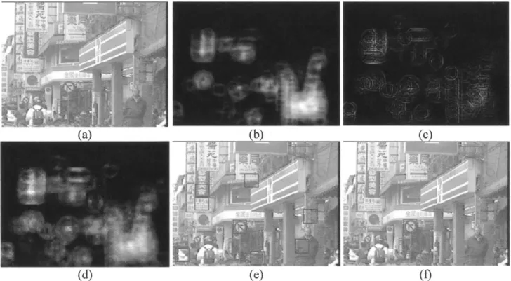
Fig. 2. An example of the road-sign detection process. (a) Original input image. (b) Color feature map of input image. (c) Shape feature map of the input image. (d) Integration map of color and shape features. (e) Result after the integration step. (f) Result after the verification step.

Fig. 1 illustrates the outline of our road-sign detection and tracking system. Once a color image [Fig. 2(a)] of a video sequence enters the system, the image is converted into hue, saturation, and intensity (HSI) channels with only the hue values of specific colors used to form the hue image . With a two-layer neural network, the color features defined as the centers of specific color regions are extracted in parallel from

. Fig. 2(a) shows an example of a road sign (no right turn) that keys off the red rim. Fig. 2(b) presents the color feature map generated by the color-feature extraction neural network. The brightness of each pixel in the map designates the possibility of being the center of a road sign based on color information.

Simultaneously, an edge-detection method is applied to ac-quire gradient values in specific color regions to construct the

edge image . Again, using a two-layer neural network, the shape features, as for the color feature, defined as the centers of certain fixed shapes, are extracted in parallel from . Fig. 2(c) presents the output of the neural network, which is referred to as the shape feature map for Fig. 2(a). The brightness of each pixel in the map denotes its possibility of being at the center of a road sign.

Fig. 2(d) shows that the color and shape features are inte-grated using a fuzzy approach to form an integration map. After finding the local maxima in the integration map, specific candi-dates for road signs are located by thresholding these maxima, as shown in Fig. 2(e). Finally, after a simple verification step, the positions and sizes of road signs are output [Fig. 2(f)] and recorded in our system to be tracked.

Conversely, in the tracking phase, to predict suitable parame-ters (image location and radius of sign) in the following image, the Kalman filter combines the detection results of image (the parameters of road signs) with the input vehicle speed at time . The results are then used to update the system parame-ters and improve the efficiency of detection.

III. FEATUREEXTRACTION

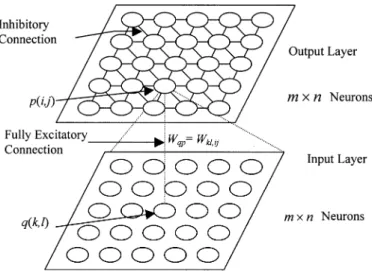
In our system, two neural networks are developed to extract color and shape features. Both of these neural networks are con-structed from two layers of neurons, one for input and one for output. The number of neurons in each layer is the same as the number of pixels in the input image. The synapses between the input and output layers are fully connected. Fig. 3 presents a sketch of the neural networks.

A. Color-Feature Extraction

Road-sign detection is more difficult under adverse weather conditions despite the fact that road signs are mainly composed of distinct colors, such as red, green, blue, and orange. The in-fluence of outdoor illumination, which varies constantly, cannot be controlled. Thus, the measured color of a road sign is always a mix of the original color and whatever the current outdoor lighting is. Moreover, the paint on signs often deteriorates with age. Thus, a suitable color model for road-sign detection is se-lected in this paper.

We believe the HSI model is suitable for road-sign detection since it is based on human color perception [11] and the color used for road signs is selected to capture human attention. Light (sun or shade) and shadows influence the values of saturation and intensity. On the other hand, hue is largely invariant to such changes in daylight [11]. For this reason, hue was chosen for the color features in the road-sign detection system.

Fig. 3. Sketch of the neural network for color (or shape) feature detection, where (i; j) is the position of neuron p on the output layer, (k; l) is the position of neuronq on the input layer, and w is the weight between neuronsq and p. The red, green, and blue (RGB) color value of an image pixel is transformed into the hue value. The saturation and intensity are not needed. The color values ( ) of a pixel at ( ) in the image are input to neuron on the input layer. If a specific color , with hue value , used in a road sign is extracted from the input image to detect a color feature, then the output of neuron is calculated from the equation at the bottom of the page is the hue of the pixel at ( ). Note that the range of is between 180 to 180 degrees and the output of neuron

is then in the range [0,1]. Neuron operates as a similarity function, i.e., the more similar the color of an image pixel is to color , the larger its output value.

The weighted output of neuron in the input layer is applied to neuron in the output layer. Depending on the shape of a road

sign, the weights between and are set

dif-ferently, since the shape information will increase the accuracy of color-feature detection.

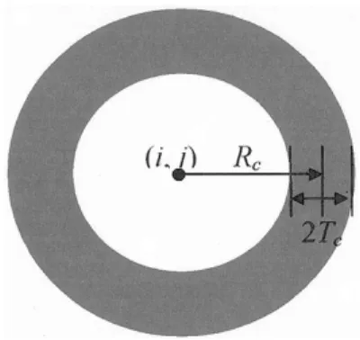
1) Circular Signs: Fig. 4 shows a circular sign with a red rim. Let be the average radius of the rim and be its half width in the image. Weight is then defined as

if if otherwise

(1)

where . and are

the inner and the outer radii of the red rim. Notice that location ( ) of neuron represents the center of the circular road sign we are focusing on and location ( ) of neuron represents the position of the pixel within the input image. If pixel ( ) falls in

where

if if

Fig. 4. Shape of circular signs.

the red rim ( ), the weight is positive. So,

if the hue value of pixel ( ) is similar to that of the red color and the output value of neuron is large, then the neuron will be greatly excited. The more red pixels that fall in the red rim region, the greater the possibility that there exists a circular red-rimmed road sign whose center is at ( ).

Now, if the distance between pixel ( ) and the center of the road sign is smaller than the inner radius of the road sign

( ), then the weight is negative. So, if there are

many red color pixels appearing inside the red rim, neuron will be heavily inhibited, since the interior of the red-rimmed road signs are typically white and black. Therefore, (1) can guide the extraction of the color features; that is, the location of the centers of the circular road signs having a special-color rim.

2) Triangular Signs: Fig. 5 shows two triangular signs with red margins. Let be the half width of the red margins, be the average height of the triangles, again in the image, and

. Then weight for upward-pointing triangular signs is defined as (2), shown at the bottom of the page. The def-inition of weight for downward-pointing triangular signs

is the same as (2) except with .

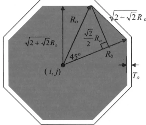
3) Octagonal Signs: Fig. 6 shows a red octagonal sign whose center is at ( ), with a white margin. Let be the distance from the center to one of the corners of the red octagon,

be the width of the white margin, ,

and . Then, weight can be

defined as the equation at the bottom of the page.

Next, for every neuron in the output layer, the net input to neuron is calculated by

net

where indices and cross all connections from the input layer to neuron .

Finally, the output of neuron is

where denotes the transfer function of neuron and is gener-ally implemented by the sigmoid function. In brief, the output value of neuron indicates the possibility of a road sign with a center at ( ).

B. Shape-Feature Extraction

Road signs have simple geometric shapes (see Table II), in-cluding circle, rectangle, octagon, and equilateral triangle. Since the shape does not vary regardless of weather or lighting condi-tions, it is a robust feature that we can exploit.

In particular, shape information assists in eliminating unsuit-able color feature points, such as the pixels of a “red” building or a “red” car (i.e., a large “red” region that is not a road sign). Shape information is still very reliable in road-sign detection despite potential occlusions or damage to some signs.

Edges are the fundamental elements that form shapes. Thus, the neurons on the input layer of the neural network for shape feature detection act as an edge detector. Let ( ) indicate the RGB color values of pixel ( ) in the color image and input to neuron on the input layer and let denote the output of neuron

. Then and (3) if if if if if if otherwise (2) if and or and or and if and or and or and otherwise.

Fig. 5. (a) Shape of equilateral triangular signs (pointing up). (b) Shape of equilateral triangular signs (pointing down).

Fig. 6. Shape of octagonal signs.

Equation (3) could be replaced by any other edge-detection equation, including Roberts, Sobel, or Laplacian. Actually, locating all of the edges in the image is unnecessary, since only specific colored edges are required.

Let be a tolerance depending on the method of edge detec-tion. Then the weight between neuron on the input layer and neuron on the output layer can be defined as follows.

As Fig. 4 depicts, let the definitions of , and be the same as in (1). Then the weight is defined as shown in (4) at the bottom of the page.

If pixel ( ) falls on the edge of the red rim, then the weight is positive. Also, if the edge magnitude of pixel ( ), which is the output value of neuron , is large, then neuron will be excited by the positive weight and the large . Therefore, the more edge pixels that fall on the edge, the higher the possibility of having a circular road sign with center at ( ).

On the other hand, where edges do not exist, the weight is neg-ative. Neuron will be inhibited if there are many edge pixels appearing in the nonedge area of a road sign. Therefore, (4)

ex-tracts the shape features that correspond to the centers of road signs having two concentric circle edges.

Similar to the weight definition of detecting the color fea-tures, we can define the weights to detect the shape features of the triangular and octagonal signs.

IV. FEATUREINTEGRATION ANDDETECTION

In this section we describe a fuzzy approach to integrating the extracted shape and color features. Here, a fuzzy approach is proposed for this purpose.

For every pixel ( ) in the input image, the membership de-gree of the pixel belonging to a road sign is defined as

where

, and ;

. Note that is a small positive constant that avoids division by 0. Here, is the output of neuron ( ) on the output layer of the color-feature-detection

neural network, is the output of neuron ( ) on the

output layer of the shape feature detection neural network, and indicates the set of neurons that are neighbors of neuron

( ), including itself. Thus, and represent the

maximum color and shape feature output at ( ) and ( ), respectively. Furthermore, and are the weights of color

and shape features. In this study, we set .

If , the color and shape features

are both at the same position ( ), then and the

value of membership function will be very large. This means that both the color and shape information confirm a road sign centered at ( ). On the contrary, if or increases, then the value of membership function will decrease.

Since an image may include more than one road sign, the local maximum of the membership function in subregions is selected to detect centers of road-sign candidates. Let the initial size of

if

if or

otherwise.

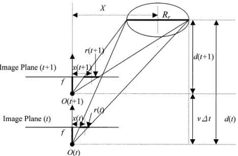
Fig. 7. Model to predict image parameters of road signs.

road signs be ; the locations of road signs is then defined as shown at the bottom of the page, where is a threshold that helps prevent the detection of weak candidates. If the output of is 1, then there is a high possibility that there is a road sign centered at ( ).

V. TRACKING

In the tracking phase, we assume that the speed of the vehicle and the physical sizes of road signs are known. If a road sign appearing in image of a video sequence has been detected, it can be utilized to predict the size and position in the following frames. This reduces the search time and space needed for lo-cating the same road sign in the next frame . For pre-dicting the location and size parameters of a road sign, we chose to implement a Kalman filter. The road signs will be continu-ously tracked until they have been recognized by the road-sign recognition system. However, the recognition system is not dis-cussed in this paper. A paper describing the recognition system has been separately submitted for publication.

Since the angle between the viewing direction of the camera and the moving direction of the vehicle is small and, to compute the values of parameters, the projected sizes and positions of road signs is for prediction purposes, an approximate derivation for the parameters can be as follows.

A. Size Prediction

As Fig. 7 illustrates, let be the physical radius of the cir-cular road sign, be the focal length of the camera, and be the

speed of the vehicle. and represent the horizontal

projection of the radius of the road sign in the images at times

and , respectively. and are the distances

be-tween the road sign and the camera axis at and in the direction of travel of the vehicle. Referring to Fig. 8, we have

and

(5) From these, we obtain

(6) Using (6), we can predict the radius , which the road sign should have in the next frame.

B. Position Prediction

Let be the lateral distance between the road sign and the

camera axis and and be the horizontal distances

in the image plane between the road sign and the center of the

image at and . Then

and (7)

From (5) and (7), we obtain

(8) From (8), we can estimate the position of a road sign projected on the image at . The vertical position of the road sign in the image can be estimated using a similar method.

if for all and

Fig. 8. Operation of the Kalman filter [16]. C. Determination of Parameters

The Kalman filter is a popular state estimation tool and Fig. 8 [16] illustrates its operation. There are two sets of equations, one for time update and one for measurement update. The first, shown on the left and known as “predictor” equations, estimates the succeeding state and error covariance. The second, shown on the right and labeled “corrector” equations, computes the Kalman gain and corrects the state and error covariance.

In these equations, represents the state vector, the a priori state estimate at step , and the a posteriori state es-timate. is the a posteriori estimate of the error covariance and is the a priori estimate of the error covariance. is the measurement vector. is the transform matrix between

and and is the transform matrix between and .

represents the Kalman gain. is the weight matrix of the con-trol input. is the control input, but this is just set to the zero vector here. and are the variances of the measurement noise and the process noise, respectively.

We define the state vector , the measurement vector , and transform matrices and as

(9) where is the focal length of the camera, is the vehicle ve-locity, is the radius of the road sign, and is the time in-terval for updating.

The image parameters of the road signs (

) are recalculated each time the Kalman filter updates , , and . These parameters of road signs provide information for detecting and verifying signs in the following image.

VI. VERIFICATION

The above integration step inevitably detects false road-sign candidates. Our system tracks all these candidates until their radii are large enough to allow verification. Once the radius of a candidate in the image is larger than 10 pixels, two rules are applied to verify whether this candidate is a road sign or not. If it passes verification and is large enough, our system will call another recognition system to recognize the candidate. If it passes but is still to small, our system continues to track it until it is large enough to pass to the recognition system. However, if there is not enough information to verify the candidate, then our system waits for more information from the succeeding frames. Our system will remove a candidate if there is not enough infor-mation to verify it in five successive frames.

All of the pixels inside the candidate are classified into one of several predefined colors. These predefined colors are those colors used in the various road signs that we wish to recognize, such as red, blue, white, and black. Pixels not matching one of these colors are marked as “don’t care.”

The hue channel can be used to classify color pixels; however if a pixel is gray, it does not work well. So, if the , , and values of a pixel are approximately the same (e.g., ,

, and ) then without computing its

hue the pixel is assigned immediately to either the “white” or “black” class.

Based on the results of color classification, the authenticity of road-sign candidates is verified. The two rules for road-sign verification are as follows.

1) The area proportions of various colors within the same road sign are fixed. For example, Fig. 9(a) shows a speed limit sign in which the red area occupies approximately 50% of the road sign and white occupies nearly 25%. 2) All road-sign shapes are symmetrical about the vertical

axis, as are most of the major colors within signs as well. Fig. 9(a) shows an example of the center of gravity of the red area, which should be very close to the physical center of the road sign.

Fig. 9. Examples of different types of road signs.

TABLE III

VERIFICATIONRULES FORVARIOUSROAD-SIGNTYPES(REFER TOFIG. 7)

: center of gravity of all pixels in road sign. : center of gravity of red (blue, white, black) pixels

in road sign. : area proportion of red (blue, white, black) pixels in road sign.

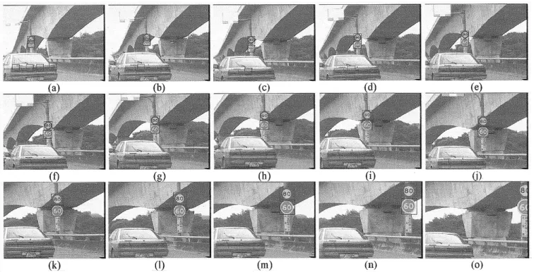
Fig. 10. Experimental results with video sequenceS . The first 15 frames of this sequence are shown in (a) to (o). The size of each image is 320 2 240 pixels and the time between two successive images is 0.2 s.

For verification, we use only a few rules, which are listed in Table III. Fig. 2(e) demonstrates the result after the integration step is applied to Fig. 2(a). It can be seen that there are eight road-sign candidates within this image. After the verification step, though, only one candidate sign is left, as Fig. 2(f) shows. Clearly, the verification rules prove greatly beneficial in elimi-nating false road-sign candidates.

VII. EXPERIMENTALRESULTS

In our experiments, video sequences from a camcorder mounted in a vehicle were used for the input to our system. The video sequences were first converted into digital images using Adobe Premiere 5.1. The size of each image is 320 240 pixels and the time between two successive images is 0.2 s.

Fig. 11. Experimental results with video sequence S2. The first 15 frames of this sequence are shown in (a) to (o). The size of all images is 3202 240 pixels and the time between two successive frames is 0.2 s.

Fig. 12. Experimental results with video sequenceS .

Fig. 10 shows the experimental results with sequence , where only 15 frames of the sequence are shown.

Consider the first frame of the sequence. All red circular road signs (and some other objects) with radius of eight pixels have been detected from the computed color and shape features. After detection, the Kalman filter corrects the estimates of the current parameters ( ) of the road signs and predicts the parameters ( ) in the following frame. Therefore, only the neighborhoods of the estimated centers, rather than the entire image, need to be examined in order to track the road signs.

If a road sign is large and clear enough, accurate verification results can be obtained, since the larger the road sign, the more complete information it provides. Alternately, verifying the road

signs too late expends too much time to track very many candi-dates. Thus, we verify a road sign only when its radius is larger than ten pixels.

Our system can tolerate several tracking mistakes. That is, if a road-sign candidate is overlooked within an image, then detected position and size are replaced by estimated position and size, as predicted by Kalman filter from previous images, until it has been detected again. However, if a road-sign candidate is lost in five successive frames, then it is dismissed.

Fig. 10(a) ( , pixels, ) shows that there

are three road-sign candidates detected by our system. How-ever, two of them are partially occluded in the succeeding image [Fig. 10(b)]. This causes a tracking error, since the actual road

Fig. 13. Experimental results with video sequenceS .

Fig. 14. Experimental results with video sequenceS .

sign cannot be correctly detected. However, the sign was recov-ered later [Fig. 10(c)]. Fig. 10(d) confirms that the road sign is correctly detected, despite partial occlusion in a few frames. The road-sign candidates were verified at the fifth image [Fig. 10(e)] of the sequence. However, since there is only one true candi-date, verification does not affect this image. Comparing frames (d) and (e) in Figs. 11, 12, and 13, the effects of verification can be observed.

Fig. 11 illustrates that our system also works when two different types of road signs exist in the same image. For clarity of presentation, the road signs are all boxed. Figs. 12 and 13 illustrate some partial experimental results with a cluttered background. Here, the red road signs are delineated with blue boxes. These examples demonstrate that our road-sign detection system can also be applied to extract road signs with various cluttered backgrounds.

Fig. 14 shows an example of road-sign detection and tracking at night. Comparing Figs. 13 and 14, we can see that the perfor-mances are the same during both day and night because road signs are also bright at night. Fig. 14(d) shows that a road sign can also be detected even it appears in an image with obvious camera vibration. From Fig. 14(g) and (h), we can observe that sometimes road signs may specularly reflect light, but this situ-ation does not affect the correctness of detection.

Fig. 15 shows several examples of detecting other types of road signs, including octagonal and upward and downward pointing triangular road signs. These images were taken under various weather conditions using different still digital and video cameras. Notably, even though some of the road signs are on a bright background, the detection results are still correct.

Running on a Pentium 4 PC (1.0 GHz), our program detects all road signs in an entire image (320 240 pixels) in

approxi-Fig. 15. Some examples of road-sign detection using still and video images.

mately 1–2 s, depending on the number of road-sign candidates and the projected size of road signs in the image. However, once a candidate is detected, the time for tracking and verifying is much faster, about 0.1 to 0.2 s, depending on the number of can-didates.

One or two seconds to detect a sign is, of course, too slow. So, we tried a simple modification to speed it up. To reduce the search time for detection, the input images were subsampled to 80 60 pixels. Our system successfully detected the road signs with a radius of approximately three pixels in the subsampled images, equal to 12 pixels in the original images. The detection time is reduced to about 0.3 s. The next section discusses addi-tional ideas for the reducing detection time.

VIII. CONCLUSION

This paper describes a method for detecting and tracking road signs from a sequence of video images with cluttered backgrounds and under various weather conditions. Two neural networks were developed for processing features derived from a sequence of color images, one for color features and one

for shape features. To extract road-sign candidates, a fuzzy approach was introduced, which integrates the color and shape features. The output of feature integration is used to detect the presence, sign, and location of road signs and candidates. A Kalman filter is then used to predict their sizes and locations in the following frame, which significantly reduces the search space for already detected objects. When an candidate sign becomes large enough, it is then verified to be a road sign or, if it fails on five consecutive frames to be verified, it is then discarded. Also, as new images come into the system, they also undergo a search for new road-sign candidates using a fixed 8-pixel radius pattern. Any newly detected candidates then go through the above process.

Experimental results indicate that our system is both accurate and robust. However, the large search space demands much time for detecting new road-sign candidates. Finally, in addition to subsampling, other ideas to reduce the search space and search time include the following.

1) As the vehicle moves the camera forward, any new road sign will appear only in the vicinity of the vanishing point

of the road (Fig. 11). If the position of the road in the image can be previously determined (e.g., using roadway detection), then the search space for road signs can be reduced significantly.

2) In three situations (Figs. 12–14), the road does not ap-pear in the image at all. However, the horizontal edges of buildings guide us to discover the vanishing point and from this we can calculate the possible region in which new road signs will appear.

3) Since the neural networks can operate in a parallel fashion, to reduce the search time, more than one CPU could be employed to implement the feature-extraction neural networks.

We hope that our future system can detect and track road signs in real time.

ACKNOWLEDGMENT

The authors gratefully acknowledge the assistance of R. R. Bailey of National Taiwan Normal University, Taipei, Taiwan, R.O.C., for his many helpful suggestions in writing this paper and for editing the English.

REFERENCES

[1] S. Estable, J. Schick, F. Stein, R. Janssen, R. Ott, W. Ritter, and Y. J. Zheng, “A real-time traffic sign recognition system,” in Proc. Intelligent

Veh. Symp., Paris, France, 1994, pp. 213–218.

[2] L. Estevez and N. Kehtarnavaz, “A real-time histographic approach to road sign recognition,” in Proc. IEEE Southwest Symp. Image Anal.

In-terpretation, 1996, pp. 94–100.

[3] J. A. Janet, M. W. White, T. A. Chase, R. C. Luo, and J. C. Sutto, “Pattern analysis for autonomous vehicles with the region- and feature-based neural network: Global self-localization and traffic sign recogni-tion,” in Proc. IEEE Int. Conf. Robotics & Automation, vol. 4, 1996, pp. 3597–3604.

[4] D. S. Kang, N. C. Griswold, and N. Kehtarnavaz, “An invariant traffic sign recognition system based on sequential color processing and geo-metrical transformation,” in Proc. IEEE Southwest Symp. Image Anal.

& Interpretation, 1994, pp. 87–93.

[5] N. Kehtarnavaz and A. Ahmad, “Traffic sign recognition in noisy out-door scenes,” in Proc. Intelligent Vehicles Symp., Detroit, MI, 1995, pp. 460–465.

[6] S. W. Lu, “Recognition of traffic signs using a multilayer neural net-work,” in Proc. Canadian Conf. Electrical and Computer Eng., vol. 2, 1994, pp. 833–834.

[7] L. Priese, R. Lakmann, and V. Rehrmann, “Ideogram identification in a realtime traffic sign recognition system,” in Proc. Intelligent Vehicles

Symp., Detroit, MI, 1995, pp. 310–314.

[8] Y. J. Zheng, W. Ritter, and R. Janssen, “An adaptive system for traffic sign recognition,” in Proc. Intelligent Vehicles Symp., 1994, pp. 164–170.

[9] A. de la Escalera and L. Moreno, “Road traffic sign detection and clas-sification,” IEEE Trans. Ind. Electrom., vol. 44, pp. 847–859, 1997. [10] D. Ghica, S. W. Lu, and X. Yuan, “Recognition of traffic signs by

artifi-cial neural network,” in Proc. Int. Conf. Neural Networks, vol. 3, 1995, pp. 1443–1449.

[11] R. C. Gonzalez and R. E. Woods, Digital Image Processing. Reading, MA: Addison-Wesley, 1993.

[12] M. Lalonde and Y. Li, “Detection of road signs using color indexing,” Centre de Recherche Informatique de Montreal, Montreal, QC, Canada, CRIM-IT-95/12–49, 1995.

[13] W. Ritter, “Traffic sign recognition in color image sequence,” in Proc.

Intelligent Vehicles Symp., 1990, pp. 12–17.

[14] G. Piccioli, E. D. Micheli, P. Parodi, and M. Campani, “A robust method for road sign detection and recognition,” Image Vision Comput., vol. 14, pp. 208–223, 1996.

[15] Y. Aoyagi and T. Asakura, “A study on traffic sign recognition in scene image using genetic algorithms and neural networks,” in Proc. IEEE

22nd Int. Conf. Industrical Electronics, Control, and Instrumentation (IECON), vol. 3, 1996, pp. 1837–1843.

[16] G. Welch and G. Bishop. (1999) An introduction to the Kalman filter. [Online]. Available: http://www.cs.unc.edu~welch/ kalmanIntro.html

Chiung-Yao Fang (A’97) received the B.Sc. degree and the M.Sc. degree in information and computer education from National Taiwan Normal University, Taipei, Taiwan, R.O.C., in 1992 and 1994, respec-tively.

She is currently an Instructor in the Department of Information and Computer Education, National Taiwan Normal University. Her areas of research interest include neural networks, pattern recognition, and computer vision.

Sei-Wang Chen (S’86–M’89–SM’97) received the B.Sc. degree in atmospheric and space physics and the M.Sc. degree in geophysics from National Cen-tral University, Taipei, Taiwan, R.O.C., in 1974 and 1976, respectively, and the M.Sc. and Ph.D. degrees in computer science from Michigan State University, East Lansing, in 1985 and 1989, respectively.

From 1977 to 1983, he was a Research Assistant in the Computer Center, Central Weather Bureau, Taipei, Taiwan, R.O.C. In 1990, he was a Researcher in the Advanced Technology Center, Computer and Communication Laboratories, Industrial Technology Research Institute, Hsinchu, Taiwan, R.O.C. From 1991 to 1994, he was an Associate Professor, Department of Information and Computer Education, National Taiwan Normal University, Taipei, Taiwan, R.O.C. From 1995 to 2001, he was a Full Professor in the same department. He is currently a Professor, Graduate Institute of Computer Science and Information Engineering, at the same university. His areas of research interest include neural networks, fuzzy systems, pattern recognition, image processing, and computer vision.

Chiou-Shann Fuh (S’89–M’95) received the B.S. degree in computer science and information engineering from National Taiwan University, Taipei, Taiwan, R.O.C., in 1983, the M.S. degree in computer science from The Pennsylvania State University, University Park, in 1987, and the Ph.D. degree in computer science from Harvard University, Cambridge, MA, in 1992.

He was with AT&T Bell Laboratories, Murray Hill, NJ, where he was engaged in performance monitoring of switching networks from 1992 to 1993. He was an Associate Professor in the Department of Computer Science and Information Engineering, National Taiwan University, Taipei, Taiwan, from 1993 to 2000, and then was promoted to Full Professor. His current research interests include digital image processing, computer vision, pattern recognition, and mathematical morphology.