A Fault Location Algorithm for Transmission Lines
with Tapped Leg —PMU Based Approach
Chi-Shan Yu** Chih-Wen Liu* Ying-Hong Lin*
*. Department of Electrical Engineering, National Taiwan University, Taipei, Talwarr
** Department of Electrical Engineering National Taiwan Umversity, Taipei, Taiwan, and Department of Electrical Engineering, Private Kuar-Wu Institute of Technology and Com-merce,Taipei, Taiwan
Absfracb-This work presents a new fault location algorithm for transmission lines with tapped legs. For the transmission lines connected with short interim tapped leg on the midway, the conventional multi-terminals fault location algorithms are inappropriate for these systems. The proposed fault location algorithm only uses the synchronized phasors measured on two-terminals of the original lines to calculate the fault location. Thus, the existing two-terminals fault locator can still be used via adopting the new proposed algorithms. Using the proposed algorithm, the computation of the fault location does not need the model of tapped leg. The proposed algorithm can be easily applied to any type of tapped leg, such as generators, loads or combined systems. EMTP simulation of a 100km, 345 kV transmission line have been used to evaluate the performance of the proposed algorithm, The tested cases include various fault types, fault locations, fault resistances, fault inception angles, etc. The study also considers the effect of various types of tapped leg. Simulation results indicate that the proposed algorithm can achieve up to 99,95”/o accuracy for most tested cases.
Index Terms-- Transmission lines with tapped leg, Fault locator, Synchronized phasor measurement units (PMUS).
I. INTRODUCTION
T
he fault location techniques can be mainly classified into one-terminal and multi-terminals based techniques. Generally, the one-terminal based techniques are simple and easy to implement. However, they are always based on certain assumptions, concerning the source impedance (i.e. the exact knowledge of the network topology during fault), fault resistance, loading, and other factors [1]. Furthermore, when multi-terminals network topologies are considered, the one-terminals based techniques are hardly to achieve accurate results. Differently, the multi-terminals based techniques [2-9] use the phasors measured at both terminals of the network to minimize the fault location errors induced from the 1assumptions in one-terminal based techniques. Thus, more accuracy results can be achieved. Additionally, when multi-terminals network topologies are considered, accuracy fault locations still can be easily calculated via the multi-terminals measurements.Since the new rights of way for transmission lines are difficult to obtain in Taiwan, transmission lines tapped by a private generating plant or load with relative short transmission lines have existed at Taipower system in recent
years. These interim connections will introduce
three-terminals transmission lines into the system. Some studies
The authors would like to thank the National Science Councd of the Republic of China for financially supporting this research rmdcr Contract
No. NSC 88-2213-E-002-070,
[2-5] have been proposed for fault location calculation of the three-terminals system. However, all of the techniques proposed in those papers need the synchronized phasors measured at all terminals of the system. Thus, when those techniques are used for the tapped lines, new installations are needed to construct those fault locators. However, since the tapped leg is always shcm and interim, the new installation of fault locators is not necessary and uneconomic. When using the two-terminals based technique [6-9] to calculate the fault location, the model of tapped leg must be constructed to compute the effect of tapped leg. However, sometimes, the model of tapped leg is not easily constructed, such as the nonlinear load model.
To avoid the new installations of fault locators or the model of tapped leg, this work presents a new fault location algorithm installed in existing fault locators. The proposed algorithm only uses the synchronized phasor measured horn the synchronized phasor measurement units (PMUS) installed at two terminals of the original transmission lines. Thus, there is no need of new installation in adopting the proposed new algorithm and the proposed algorithm is appropriate to the interim tapped transmission lines. In addition, since the model of tapped leg is not used in the proposed algorithm, the fault location algorithm can be easily extended to any types of tapped leg (such as generator, or load). When two-terminals algoritluns are used to calculate the fault location of tapped system, fault locator must decide whether the fault occurs on left side or right side of the tapped leg. In this paper, a selector is presented to choose the correct side of the tapped leg.
The rest of this paper is organized as follows. Section II begins by describing the theory used to determine the fault location of a tapped connected tmnsmission lines. Then, this section proposes a selector for selecting the correct faulted sides with respect to tapped leg and proposes a method of double-checking the input fault types. A 345 kV sample system is used to evaluate the accuracy of the proposed algorithms with respect to different fault types, fault locations, and fault resistance. Next, Section III presents the simulation results of the performance evaluations. These simulation results come horn extensive EMTP [12] tested case. Meanwhile, Section IV discusses some special phenomena from the simulation studies in detail. Conclusions are finally made in Section VI.
11. PRINCIPLES The proposed algorithm is derived using assumptions:
1. the fault impedance is pure resistance.
2. the fault type is a prior input,
The assumptions above are common in the literature dealing with the fault location issue.
SendingEr,d ,-. .–. ..–... –..., Reed@End
Ss1
~ —
DZL — L! TL
+
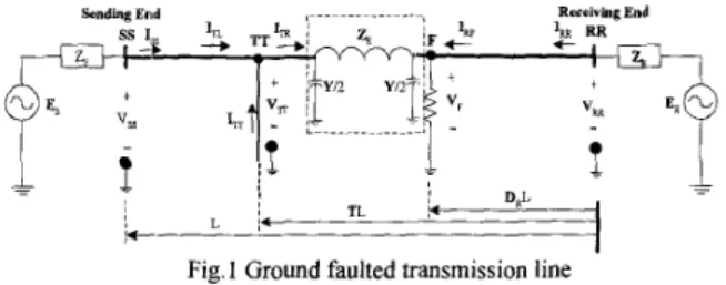
Fig, 1 Ground faulted transmission line
A. Fault Location Algorithm
To illustrate the ideas of the proposed algorithms, this work considers the three-phase transposed transmission line with tapped legs shown in Fig. 1. The subsystem connected behind the tapped leg can be generators, loads, or combined systems. The tapped leg is connected at a distance of T [p.u.] away tlom the receiving end of the transmission lines and labeled as TT. Meanwhile, SS and RR label the sending and receiving ends of transmission line, respectively. Fig. 1 displays that the quantities at each end are all vectors of phase voltages and currents. The long distance distributed transmission line model is used in EMTP simulations and the development of fault location algorithms.
The voltages and currents at a distance x kilometers away fi-om the receiving end are governed by the partial differential equations: L3v ~l+Lg —= 13x 3 (1) ~= GV+C— at
where both V andI are3 x 1 vectors. R, L, G and C are all 3 x 3 transposed line parameters matrices with similar forms such as:
[1
Ls L~ L~
L= L~ Ls L~ (2)
L~ L~ Ls
Under sinusoidal steady-state condition, (1) can be rewritten as i?v ~1 —. ax aI (3) —=YV ax where Z = R +jmL and Y = G +j@C.
To decouple inter-phase quantities, a suitable transformation, referred to as symmetric component transform [13], is given as follows:
[1[1 Va Vo v~ =s v, Vc v~ [H] 1, 10 lb =S 11 (4) Ic 12
where O, 1, and 2 respectively represent the zero, positive and negative sequence symmetric components of the voltage and current quantities, and the sequence transformation
matrix is as follows:
[1 111
s=lct2ci (5)
la a2
where a = IZ1200. Substituting (4) and (5) into (3) gives the following sequence equations:
!!!!w.
Z0121012 ax a1012– Yo12v~12 —_ ax (6)where Z012 and Y012 are the sequence impedance and admittance matrices, respectively. Both Zolz and YOIZare diagonal matrices, and the diagonal entries of matricesZO12
andY012 are(ZO, Zl, Z z)and (YO,Y 1, Y J, respectively.
Thus, (6) represents three decoupled sequence systems whose solutions can be obtained as
Vm = Am exp(ymx)+Bm exp(–ymx)
Im = [Am exp(ymx)+Bm exp(–y~x)]/Z, ~ (7)
where the subscript m denotes O, 1 and 2 sequence variables, zC~= J= denotes the characteristic impedance, and y~ =~~is the propagation constant. Meanwhile, the constants Am and B~ can be determined by the boundary conditions of voltages and currents measured at both ends of the line.
Since the fault location with respect to the tapped leg is unknown prior to fault location calculation, the proposed fault location algorithm will fwst calculate two locations via subroutines 1 and 2 simultaneously. These two faults are assumed to occur at right and left sides of the tapped leg, respectively. Then, a selector is developed for exactly distinguishing the true fault side.
Subroutine 1 – Fault location for the ri~ht side of the tapped leg
In this subroutine, Fig. 1 is still used for investigation. Fault location is assumed to be located on right side of tapped leg at a distance of DR [p.u.] away tlom the receiving end of transmission lines and labeled as F, where subscript R denotes the variables defined on right side of tapped leg. Meanwhile, the tapped leg is connected at a distance of T [P.u.] away fkom the receiving end of the transmission lines and labeled as TT. The transmission lines in Fig. 1 are divided into two line sections with respect to the tapped leg. Both of them can be regarded as transmission lines without tapped leg. When the voltages V~T on tapped leg and currents ITR on right side of tapped leg are known, fault location DR can be calculated using conventional two-terminals techniques [6-9]. The voltages VTTon tapped leg and transmission line currentITLon lefi side of tapped leg can be calculated using the line section between SS andTT
incorporates with the boundary conditions of VSS and 1SS. However, due to the uncertainties of tapped leg, the injection currents ITT from tapped leg are unknown and the transmission line currentITRon right side of tapped leg are also unknown. Thus, the conventional two-terminals techniques can’t be directly used in this system.
In this work, the Gauss-Seidel numerical method is used to calculate the fault location. In the line section between
tapped leg and receiving end, the unknown variables are currents ITRand fault location DR (or fault resistance RFR, fault voltage V~~. Using a two-ports model to represent the line section between TT and F, the resulting diagram is illustrated in Fig.2, According the circuit theory and assumption constraint, two groups of equations are obtained as follows:
Group- 1: Network equations Fl( I~R,DR,8)=0 Group-2: Constraint equations
Fz( ITR,DR, e)=O
where 8 are the known variables, such as Vss, Vm, VTT,etc., and ITR,DR are the unknown variables. Group-1 equations are obtained from the two-ports network enclosed by dashed line in Fig. 1. Group-2 equations are obtained 120m the assumption of pure resistance fault impedance. Since the simultaneous equations of Group-1 and Group-2 are nonlinear, numerical method [14] is needed to find the solutions of IT]<and DR.
In this work, the Gauss-Seidel numerical method is used. The calculating procedures are arranged as follows:
1! Give an ‘initialvalue of D ~ (superscript 1 denotes the initial valhteof the fwst iteration).
2. Substitute D ~ into Group-1 equations to calculate I ~~. 3. Substitute I ~~ into Group-2 equations to calculate D ~. 4. Repeat steps 2 and 3 to calculate the final results of ITR
and DR.
For saving the space, only the three-phase-shorted fault is adopted as the example to demonstrate the above procedures. Other types of faults can also be easily calculated via the proposed procedures. Three-Phase-Shorted Fault: Group- 1 equations: Vml+-IWIZC1 VF1‘— 2 exp(yl DRL) + VM1– Im~lZcl 2 — exp(–yl ~ L)==O ITR1– (VTT-V~l)/ZE1+VT~lXyl/2 = O Vml -I-ImlZcl IF1 +[— ~ exp(yl DRL) Vml – Iml;cl — —exp(–yl DRL)]Z,~~ 2 V~~l+ ITILIZC1 -[ —exp(yl DRL) 2exp(y1TL) VTT1–ITRIZC1 — —exp(–yl DRL)]Z~\ = O 2exp(yl TL) Group-2 equations: Re{I,l(DR)}X Im{V~l(DR)} –Re{V~l(DR)}x Im{I~l(DR)} = O (8) (9) (lo) (11) where subscript1denotes the positive sequence components, Re{ . } and Im{ . } respectively denote the real part and imagimuy part, (8)-(10) are obtained from transmission lines network model, (11) is obtained from the fault impedance assumption, and VT1is expressed as
VTT1=Vssl+ IsslZcl 2
exflyl (1–T)L]
(12) + ‘ssl– ~slzcl exfl– yl (1– T) L]
Using the above two groups equations and the procedures mentioned above, fault location of DR can iteratively be calculated.
Subroutine 2 – Fault location for the left side of the tamed leg
When the fault occurs on the lefi side of the tapped leg, substituting the relations Vss=Vm, Vm=Vss, lss= – Im and Im= - Is~into the above equations, and thus obtaining a new per-unit fault location (denoted as D’) in relation to the reference x = L. When x = O is taken as the reference point, the final per-unit fault location can be computed from D~ = 1- D’, where subscript L denotes the variables defined on left side of tapped leg.
So far the proposed scheme has only generated two solutions of DRand DL, and which one is the exact fault location remains undetermined. A selector that can easily resolve the mentioned problem will be overlooked here and dealt with later.
B. Fault Side Selector
The resulting solutions of DR and DL can be divided into the following five conditions:
1. Both DRand DLare fix values e [T, O]. 2. Both DRand D~ are fix values e [1, T].
3. DRcannot be found and DLis a fix value e [1, T]. 4. DLcannot be found and DRis a fix value e [T, O]. 5. DR= [T, O],and DL= [1, T].
Since the computation of fault locations DR and DL bases on the assumptions: DR●[T, O]and DLs [1, T], the solutions
of DL and DR in condition 1 and condition 2, respectively, violates the assumption. Meanwhile, both condition 3 and condition 4 have only one feasible solution, respectively. Thus, the correct solutions of condition 1 to condition 4 can be easily chosen. However, the selecting of condition 5 remains confusedly. The proposed selector is dedicated for this case. In our investigations, in condition 5, the fault resistance RF of the correct side is positive, and the fault resistance of the incorrect side is negative. Therefore, the selecting criterion for condition 5 can be obtained as follows:
The fault location of the calculated set [DR, DL] that corresponds to positive RFis selected as the correct solution. C.Demonstration of Fault Side Selector
Herein, the proposed selector is proved via the short distance transmission lines model shown in Fig.2. The tapped leg is connected at a distance of T [p.u,] away from the receiving end of the transmission lines and labeled as TT. The subsystem connected behind the tapped leg can be generator or load. Fault is assumed occurs at the right side of the tapped leg. The per-unit fault location D [p.u.] is the correct fault location and the per-unit fault location D’ [P.u.] is assumed to be the incorrect fault location, where the fault location II and D’ are on the right side and left side of tapped leg, respectively. Using KVL, the relations of VSSandVRR
V~~=(l– T)LZ&+(T – D)LZ&~+I~~)+V~
=(1 – T)LZ&~+(T-D)LZ&+I~~)+(I~~+Im+I~~)R~ ‘(1 – D’)LZ&+ V;
=(1 – D’)L/ZJ~~+(I~~+Im+1~ ) Rfi (13)
Vm=TLZ~Im+( D’ – T)LZ~(Im+ I!m )+ V;
= TLZ&&( D’ – T)L~(Im+ Ifi )+(I~~+Im+1~ ) RF =DLZJm”-V~ =DLZ&+(I~~+Im+I~JRp
Vm=TLZJm+( D’ – T)LZ~(Im+ 1~ )+ V;
= TLZ~IW+( D’ – T)LZ~(Im+ 1~ )+(I~s+Im+ Ifi ) R\ =DLZJm--V~ =DLZ&+(I~s+Im+I~~)R~ (14) rewriting (13) as
0=( D’ – T)LZJss+(T – D)LZL(Iss+ITT)
+ (ISS+Im+IrT)RF– (Iss+I~+ Ifi ) R ~ (15) Meanwhile, (14) is rewritten as
0=( D’ – T) LZL(Im+ 1~ )+(T – D)LZLIm
––(Is~+Im+ITT)RF+(Iss+Im+ 1~ ) R~ (16)
where (Iss+Im+I~T)=I~is the fault current of the correct side, (Iss+IM+ Ih )= I; is the fault current of the incorrect side. From (15) and (16), the following relation is obtained
O=(T– D)I~+ ( D’ –T) 1; (17)
Since (T – D) and ( D’ – T) are all positive and real constants, the phase difference between IF and 1~ must be 180 degrees. Meanwhile, due to the pure resistance assumption on fault impedance, the phase difference between V~ and V; must be zero or 180 degrees. The zero degree of phase difference indicates RFR; <0 or R; <0, since RF must be positive. The 180 degrees of phase difference indicates RFR; >0 or R& >0. From conventional circuit theory, the 180 degrees of phase difference between VFand V+is impossible, since the phase difference between sending end and receiving end is much less than 180 degrees. The possible phase difference between VF aridV; is zero degree. Thus, when condition five occurs, the fault location with positive fault resistance is selected as the correct solution.
6’
SnbsystemFig.2 Transmission line for demonstrating selecting algorithm
When the fault occurs at the left side of tapped leg, same results can be obtained by the similar procedures used in above.
D. Fault Location Calculation on Tapped Leg
In this work, the proposed algorithm only concentrates on the fault location calculation of the original transmission lines, and the tapped leg is assumed to be very short or interim. However, when the fault location calculation of the
tapped leg is necessary, the fault location still can be calculated via the synchronized measurements from two-terminals of the lines. Before calculation the fault location on tapped leg, the decision of tinding whether fault occurs on the tapped leg or the original transmission line. The fault location algorithm proposed in this work incorporate with the two-terminals based fault location algorithm [9] can be used for identifying of this condition. When fault does not occur or fault occurs on the tapped leg, the results calculated Ilom the algorithm proposed in this work cannot be found. In addition, the results calculated from the conventional tsvo-terrninals based algorithm [6-9] will equal or near to the tapped leg location. Thus, when both of the above conditions occur, the voltageVTTon tapped leg and the current ITTon tapped leg can be calculated from basic circuit theory and the synchronized boundary conditions of[Vss, 1ss, Vm, Ire].
Additionally, the well-known one-terminal based technique [1] can incorporate with the phasors of [VTT,ITT]for fault detection and fault location calculation of the tapped leg
III. PERFORMANCE EVALUATION
A. Algorithm Test
Herein, the proposed fault location algorithm is evaluated via some case studies. The parameters of simulation sample are listed in Table I. Meanwhile, transmission line connects a tapped leg located at 45 km (q = 0.45 p.u.) away from the receiving end of the protected line. All the systems are simulated by EMTP. In order to achieve more accurate results, the phasors are estimated using the SDFT [14-15] filtering algorithm working at 32 samples per cycle. The total simulation time is 200 milliseconds and the error of the fault location is expressed in terms of percentage of total line length. The fault locations, fault resistances and the phase angle of fault currents are computed fi-omsubroutine 1 and subroutine 2 simultaneously at 3 cycles after fault inception.
TABLE I. PARAMETERS OF THE SIMULATIONSYSTEM
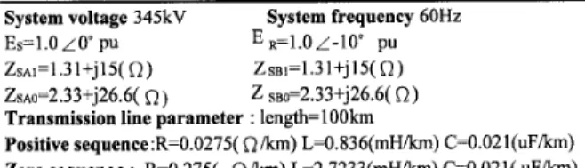
System voltage 345kV System frequency 60Hz
Es=l.OZW pU ‘R=l.O/-l~ pU
ZSAl=l.31+j15(~) .zSB1=l.3]+j15(~) ZsA0=2.33+j26.6(Q) Z sBn=2.33+j26.6(Q) Transmission line parameter : length=100km
Positive sequence:R=O.0275( Qikrn) L=O.836(mH/km)C=O.021(uFikIn) Zero sequence : R=O.275( Qikm) L=2.7233(rnH/km)C=O.021(uFikm) Generator Tvrre Tatmed Leg Tests:
In the following test cases, a generator is connected behind the tapped leg and modeled as a voltage source ET. The source impedance of ETis equivalent to that of Es in Table I. The length of the tapped leg is very short and equal to 5 km.
Case 1:Fault Location Algorithm Test – Small Fault Resistance
A simple case is used to demonstrate the proposed fault location algorithm. Assume that a single-line-to-ground fault occurs at70 km (D =0.7 p.u.) away from the receiving end of the line. The fault resistance is assumed to be 1Q. The phase of ES leads the phase of ET by five degrees. The results of subroutine 1 and 2 are written as follows:
Subroutine: DI,=0.7001(p.U.),R~=l.0274Q, Arg(I~)=l .662(rad)
Since D~ cannot be found in subroutine 1, the correct fault location is easily chosen as D=O.7001 (p.u.) (error=O,OlYo). Case 2:Selector Test – Fault occurs at left side of tapped leg A special case is u:;ed to demonstrate the accuracy of proposed selector. Assume that a three-phase-ground fault occurs at 90 km (D = 0.9 p.u.) away from the receiving end of the line. The fault resistance is set as 150Q. The phase of Es leads the phase of ET by five degrees. The results of subroutine 1 and 2 are written as follows:
Subroutine 1: D~= Cl.1344 (p.u.), RF=– 105.81Q, Arg(l~)=– O.1922(rad)
Subroutine: DL,=0.8993(p.U.),R~=150.26Q Arg(l~)=2.949(rad)
Since the fault resistance is negative in subroutine 1, the correct fault location is chosen as D=O.8993 (error=O.07%). Notably, the phase difference of IF between subroutine 1 and subroutine 2 is 3.14 12(rad), and approximates to 180 degrees. The difference between 3.1412 and 180 degrees (3. 1416) is very small and is induced fi-omthe short distance transmission lines assumptions in the demonstration of previous section.
Load Tvpe Tapped Le~ Tests:
In the following case, a load is connected behind the tapped leg. The length of the tapped leg is also 5 km. Case 1:Fault Locaticm Algorithm Test – Small Fault Resistance
A simple normal case is used to demonstrate the proposed fault location algorithm. Assume that a line-to-line fault occurs at 30 km (D = 0.3 p.u.) away horn the receiving end of the line. The fault resistance is set as 1Q. The load connected behind the tapped leg is modeled as 30MW+21 Mvar at nominal voltage. The results of subroutine 1 and 2 are written as follows:
Subroutine: D~=0.3001(p.u.),R~=l .0091Q, Arg(IJ\=l .4976(rad)
Subroutine 2:D~= 0.;!936 (p.u.), RF=– 3.73f2, Arg(I~l= – 1.6361(rad)
Since D~ violates the assumption of subroutine 2, the correct fault location is easily chosen as D=O.3001 (p.u.) (error=O.O1%).
Case 2: Selector Test--Fault occurs at right side of tapped leg
Assume that a three-phase-ground fault occurs at 10km (D = 0.1 p.u.) away from the receiving end of the line. The fault resistance is set as 100Q. To demonstrate the possible of condition 5 in this case, an special but unreasonable load is assumed to be connected behind the tapped leg and modeled as 100MW+70MVW at nominal voltage. Due to the extremely large power consumption of this load, the tapped leg can still sink current in fault period.
Subroutine 1: D~=O.1001(p.u.),R~=99.99Q, Arg(I~)=2.6863(rad)
Subroutine 2: D~= ().4651 (p.u.), R~=–4.09s2, Arg(l[~)=– 0.4549(rad)
Since the fault resistance is negative in subroutine 2, the correct fault location is chosen asD=O.1001 (error=O.O1‘?40).
Notably, the phase difference of IF between subroutine 1 and subroutine 2 is 3.1412(rad), and approximates to 180 degrees.
B. Statistical Evaluation
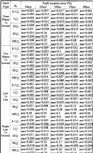
This subsection evaluates the proposed fault location algorithm with over 1000 test cases obtained from the EMTP simulator. It considers different fault types, resistances, locations, and inception angles as statistical tests. Meanwhile, both generator connected tapped leg and load connected tapped leg are considered. The same transmission line model in Table I is still used. The tapped leg connects at 45 km away fi-om the receiving end of the line. For the generator connected tapped leg, the phase of ES leads the phase of ET five degrees. For the load connected tapped leg, the load is modeled as 30MW+2 lMvar at nominal voltage. Table II summarizes all of these results. The fault inception angles are O, 45, 90, 135, and 180 degrees in relation to the zero cross of a-phase voltage. For saving space, all of the fault location errors are calculated as the average errors for different inception angles and different kind of tapped legs. In Table II, variable Ave is the average fault location. For comparison, variable max is the maximum fault location error in ten fault locations. In all cases, the maximum error is 0.6% and the average error is about 0.039?40.Additionally, if only considering the fault resistance less and equal 10W, the maximum error reduces to O.17°/0and the average error is only 0.014°4, mi7 Type ‘Huee ‘bases To imund Two ‘bases To hound Lure To Lme
1~1,12 U. >lA1l>llLAL lbS1lNti Uk lHk.4LLjUKll HM
I Faultlocationerror(%) I
“YO”m==”l
0,1~ a-o.oo1 ave=O.007ave=O.017 ave=O.007 we=O.ool IIMIX=O.001 IIM=O, O12 mm=O.026~mm==.011 IIMX=O.001 lQ ave=o.oo3 we=O.007 ave=o.o 10 iwe=O.004 ave=o 002 max=0,004 max=OO11 max=O.015 max=O.006 mm=O.00: 100 “~o””q ‘V’=0”35 ~~=o.oo6 ‘V’=0,014 ‘v’+ol~max=O.O1 max=O.038 max=O.008 maFO.O15 max=0.02 CJ”Q ave=O.014 /ave=”. 16 ave=O.055 ave=O.O1 ave=O.00$
max=O.026ima~O.25 max=O,IO max=O.O19max=O.O1~ 100Q “-”.””8 av’=ozz ave=0,083 rwe=O.08 ave=O.009 mafiO.015 max=O.47 mrix=0,16 maFO. 12 nMx=O.O1’ 0.1 Q ‘“=0.003 ave=ooo9 ave=oo49 av=” “12 ave=oJ303 max=o.oo7 max=O.021 max=O.1 max=0,021 max=0.00! IQ ave=o.oo2 ave=o.o14 ave=o.037 ave=O.006 ave=O.002
max=O.005 max=O.032 max=O.063 max=O.013 nMx=0.00z
Inn av~” ““ 1 we=O.014 ave=0.049 Iave=0,008 ave=O.0~ “““ ~maFo,0132 IIMX=O.023 IIW=0,083 maFO.022 max=O.004
a
5“ Q We=o.ool ive=O.O11 ave=o 045 ave=O.005 ave=O 001 max=O.002 max=O.027 mar=,068 max=O.O1 max=O.002 1Ml n Iave=o.oo2nVe=O.O14ave=O.047ave=O.008nve=O.001
=&II
‘““‘JO.I Q WFo.oolma=O.002max=O.032ave=o.olj max=0,080-o.038 max=O.021av’=o.oog ave=o.oolmax=O.002max=O.001 mIIx=O,035 max=0,057 msx=O.O19 mtrx=O.002 ave=O.002 ave=O.008 ave=O.013 ave=O.041 .we=O.001 ma~O.003 mar=.015 mafiO.025, marO.056 maA.002 100 w=o olc ave=o.o’21 ~ve=o.osz Iav’+oo7 ave=o.ol 1
h--”--
‘“”––
‘“ max=0,027 maFO.034 max=O.055 mux=O.014 m9x=0.015 aviFO.021 ave=O.098 ave=O 19 ave=O.14 ave=O.067
~ ‘-L
max=O.046 max=O.11 max=O.28 ma~O. 18 max=0.092 iIOOQave=O.05 ave=O,54 ave=O.3 ave=O.09 ave=O.04
max=O.12 IIMX=O.6 max=O.6 mar=. 16 max=O.053 i 0.10 ave=O.020 we= O.003 ave=O.039 ~ave=O O14 ave=O.01 1
~--+
max=O.040 max=0,006 max=O.069Imax==.O19 gO.029 ::! lQ’ ave=0,008 ave=O.008 ave=O.036 ,ave=O.012 ave=O~O09
‘IIWF0,009 mar+.012 mIaFO.069’m-4.018 IIV4X+.021
‘;o&+--~~nd 10 ~ av~O.O 11 ,ave=O.O13 ave=O.065 ave=O,O13 we=0.006 mri~0.026’ IIMX=O.024max=o,17 ma~O.022 mafiO.O13 ave=O.001 ave=O.12 ave=O.11 ave=0,055 ave=0,004 max=O,O18 IUU==.28 max=O.20 max==.090 max=0.006
ave=O.16 ave=O.12‘-we=O .007 ;max=O.022imax=O.25 max=O27 ma~O. 16 max=O.O11
IV. CONCLUS1ONS
This work has successfully proposed a new fault location algorithm for transmission lines with tapped legs. For the transmission lines tapped with a short or interim transmission line, three-terminals fault location algorithms are inappropriate and uneconomic for these systems. The proposed algorithm does not use the real-time measurements of the tapped legs. Thus, the proposed fault location algorithm is appropriate for these systems. Meanwhile, the proposed fault location algorithm does not use the model of the tapped leg in fault period. Thus, the proposed fault locator can be easily applied to transmission lines with any type of tapped leg, such as generator, load or combined systems. To select the correct fault location with respect to the tapped leg, the fault side selector also has been presented in the work. The simulation results show the proposed fault location algorithm and the selector can easily produce and choose accurate fault location result.
[1] [2] [3] [4] [5] [6] [7] [8] [9] [10] [11] [12] [13] [14] V. REFERENCE
L. Eriksson, et al, “An Accurate Fault Locator with Compensation for Apparent Reactance. in the Fault Resistance Resulting from Remote-End Infeed,” IEEE Trans. on PAS, Vol. PAS-104, N0,2, Feb. pp,424-436, 1985,
A, A. Girgis, D, G, Hart. and W. L. Peterson, “A New Fault Location Technique for Two- and Three- Terminal Lines”, IEEE Trans on Power Delivery, VO1.7,No.1, January, pp. 98-107, 1992.
R. K. Aggarwal, et. al., “A Practical Approach to Accurate Fault Location on Extra High Voltage Teed Feeders”, IEEE Trans., PWRD-8 (3):pp,PWRD-874-PWRD-8PWRD-83> 1993.
Abe Masayuki, “Development of a new Fault Location System for Multi-terminals Single Transmission Lines,” IEEE Trans., PWRD-10 (l)pp.159-168, 1995.
Qiww Gong,et al, “A Study of the Accurate Fault Location System
for Transmission Line Using Multi-Terminal Signals”, IEEE Winter Meeting, 2000.
A. T. Johns, et al, “Accurate Fault Location Technique for Power System Lines”, IEE. Proc. Pt.C, Vol. 137, pp.395-402, Nov. 1990. M. Kezunovic, “An Accurate Fault Location Using Synchronized Sampling at Two Ends of a Transmission Line, “ Applications of Synchronized Phasors Conference, Washington, DC, 1993. D. Novosel et al, “Unsynchronized Two-Terminal Fault Location Estimation,” IEEE PES Winter Meeting, New York, Jan. 95WM025-7 PWRD, 1995.
J. -A. Jiang et rd, “AU Adaptive PMU Based Fault Detection/Location Technique for Transmission Lines Part I“, IEEE Trans. on PWRD, VO1.15,No.2, pp.486-493, 2000.
J. –Z. Yang aud C. –W. Liu, “A precise calculation of power system frequency and phasor”, IEEE Transactions on Power Delivery, Vol.15, No.2, pp.494-499, 2000.
J. –Z. Yang and C, –W, Liu, “Complete Elimination of DC offset in current signals for relaying applications”, IEEE Winter Meeting,
2000.
Dommel H., Electromagnetic Transient Program, BPA, Portland, Oregon, 1986,
C. A. Gross, Power System Analysis, John Willey, 1986.
John R. Rice, Numerical Methods, Software, and Analysis, Academic Press Inc., San Diego, 1993,
VI. BIOGRAPHIES
Chih-Wen Liu was born in Taiwan in 1964. He received the B.S. degree in Electrical Engineering from National Taiwan University in 1987, and M.S. and Ph.D. degrees in electrical engineering from Cornell University in 1992 and 1994. Since 1994, he has been with National Taiwrm University, where he is associate professor of electrical engineering. He is a member of the IEEE and serves as a reviewer for IEEE Transactions on Circuits and Systems, Part 1. His main research area is in application of computer technology to power system monitoring, operation, protection and control. His other research interests include GPS time transfer and chaotic dynamics and their application to system problems.
Ying-HongLin wasborn at Taipei, Taiwan, in 1970. He received his B.S. degree in electrical engineering from Taiwan University of Technology in 1995 and M.S. degree horn National Taiwan University in 1999. He is a candidate for the Ph.D. degree in the electrical engineer department at National Taiwan University, Taipei, Taiwan. His interested researches are the application of GPS and PMU in power system,
Chi-Shan Yu was born in Taipei, Taiwan in 1966. He
received his B.S. and M.S. degree in electrical engineering from National Tsing Hua University in 1988 and 1990, respectively. He is a candidate for the Ph.D. degree in the electrical engineer department at National Taiwan University, Taipei, Taiwan. His current research interests are computer relaying and transient stability controller.