Minimax design of two-dimensional parallelogram filter banks

(1)

~ ~ _ _ _ _

Minimax design of two-dimensional parallelogram

filter banks

C.-K. Chen J.-H. Lee

Indexing terms: Parallelogram filter banks, Minimax design

Abstract: The authors present a technique for the

minimax design of two-dimensional (2-D) parallelogram filter bank (PFB) systems with linear-phase analysisjsynthesis filters. To achieve perfect reconstruction, the required analysis filters must have parallelogram-shaped frequency responses. In general, the original design problem is found to be an optimisation problem with nonlinear constraints. The authors present a linearisation approach to reformulate the design problem.

As a result, updating the filter coefficient vector at

each iteration for the original design problem can be accomplished by searching the gradient of the linearised optimisation problem. They further present an efficient method based on a modified Karmarkar’s algorithm for computing the required gradient vector and finding the required step size analytically. Therefore the filter coefficients can easily be computed by solving only linear equations at each iteration during the design process. The effectiveness of the proposed technique is shown by computer simulations.

1 introduction

Multirate filter banks have received much attention, as they find applications in many areas, such as subband coding of speech signals [ I , 21, communication systems

[3,4] and short-time spectral analysis [ S , 61. Their applications have been extended to two dimensions (2-D), e.g. for the subband coding of images [7, 81, which has been recognised as an effective technique for high quality imagG coding at low bit rates; directional decomposition of image data [9], which has been found to be useful for several image processing applications [IO] ; determining the direction of arrival of plane wave and the removal of ground roll when processing seismic data [ I I], and 2-D short-time spectral analysis [I 21. 2-D multirate filter banks with maximally decimated subband channels have also been considered [13, 141.

The 2-D filter banks previously considered for applications were separable filter banks [7]. This is because the required operations for their implementation can be performed in each dimension separately, and hence the required implementation complexity is very low. ic, IEE, 1995

Paper 2091K (E4, E5). first received 15th August 1994 and in revised

form 30th May 1995

The authors are with Department or Electrical Engineering, Room 517, 2nd Building, National Taiwan University, Taipei, 106 Taiwan, Repub- lic of China

220

However, it has been shown that nonseparable 2-D filter banks are also very important, and are required in some applications [lo, 151.

Several nonseparable filter banks have been considered for their applications in multirate systems [13]. Among these nonseparable filter banks, 2-D parallelogram filter banks (PFBs) are useful for applications in which 2-D signal data are decomposed into directional components, e.g. the extraction of the directional image components required for the directional subband coding of image data [lo]. It has been shown [9] that the

required lowpass analysis filters must have a parallelogram-shaped passband response ’ in order to decompose an image into wedge-shaped spectral regions. Methods for designing 2-D PFBs have been presented. In [9] a method was proposed based on a change of variables which transforms the checkboard-shaped filters generated by a pair of 1-D QMFs to a 2-D PFB with arbitrary passband directions. Although this design method is very simple and straightforward, the resulting 2-D PFB is in general not optimal.

In this paper, we consider the minimax design of 2-D PFBs. As the filters required in each subband of a 2-D PFB must possess a linear-phase response, especially for many applications related to image coding [17], the design problem is thus formulated to constrain all the analysis/synthesis filters to have a linear-phase response. At each iteration during the design process, the resulting nonlinear constrained optimisation problem is tackled by first linearising the nonlinear constraints. Only a first- order approximation for linearisation is considered. Then, an efficient method based on the use of a modifi-

cation of Karmarkar’s algorithm [I81 is developed for updating the filter coefficient vector. The main computational load required during the design process is the solu-

tion of linear equations. Moreover, an analytical formula is also presented for calculating the step size required at each iteration. Therefore, the need for any line search procedures can be avoided during the design process. This leads to tremendous savings in computational burden. Computer simulations show that very satisfactory design results can be obtained efficiently using the proposed technique.

2 Principles of 2-D PFBs

The system structure of a general two-channel 2-D PFB is shown in Fig. 1, where the decimation/expansion

This work was supported by the Taiwan National Science Council under Grant NSC84-2213-EOO2-

I

046.

t - -

(2)

matrix

M

is determined

by

the nominal

passband

region

.of the lowpass analysis filter Ho(z,, z2). For the case. of

-

analysts system- -synthesis systern-

System structure o f a general two-channel 2-D P F B

Fig. 1

2-D PFBs, H,(z,, z2) possesses a parallelogram-shaped passband region given by

{ --n

<

M , , o ,

+

Mz1w2

<

n)

n { - x < h f 1 2 w l + M z z w , < n ) (1) The corresponding matrix M is required to be as follows c131

It has been reported that four different parallelogram- shaped band-splitting structures are required for applications to directional frequency component decomposition. Fig. 2 shows the four parallelogram-shaped band-

a b C d c Category C d Category D Fig. 2 U Category A b Category B

<our parallelogram-shaped band-splittlng structures

splitting structures used for eight-band decomposition. Let a 2-D PFB whose lowpass analysis filter has a nominal passband region shown by Figs. 2a, 2b, 2c and 2d, respectively, be designated as categories A, B, C, and D. Based on expr. 1 and eqn. 2, we have the associated decimation/expansion matrix for each category of the 2-D PFB as follows

M e = [ - 1

'1

1 M , = [ y (3)

Each of these matrices is a 2 x 2 nonsingular matrix and is used to indicate the 2-D decimation operation. Since the value of the determinant for each matrix is equal to 2,

I E E Proc-Vis. Image Signal Process., Vol. 142, No. 4, August I995

the

corresponding

decimation

operation

is

performed

with a decimation ratio equal to 2.

For category A, the relationshp between the input and output for the 2-D PFB is given by

X(z,, 2 2 ) = iCHo(z,, Z2)F,(Z,, 2 2 )

+

Hi(zi, Zz)Ft(Zir zz)IX(zi, ZZ)

+

iCHo(z1, -z2)Fo(z1r

4 +

H,(z,, -z,)F,(z,, Z Z ) l X ( Z , ,

-4

(4)

The first term of eqn. 4 represents the response of x(nl, n2) passing through a linear-shift invariant system with a transfer function given by [H,(z,, z,)F,(z,, z z )

+

H,(z,, z2)F,(z,, z2)]/2. while the second term represents the aliasing component induced by the 2-D decimation operation. If we set the following conditions:

Fo(z,, z2) = 2H,(z,, -z2)

F,(z,, 2 2 ) = -2H,(z,,

-4

and (5)

Then the aliasing component in eqn. 4 can be eliminated and the equation becomes:

- Hi(zi, ~z)Ho(zi, -z2)1X(z13 zi) (6) Next, we note from Fig. 2 that constructing a PFB for category A requires H,(z,, zz) = H,(z,, -z2) or the cor- responding impulse responses h,(n,, n 2 ) = ho(n,, n,)(

-1)"2, where ho(nl, n2) and h,(n,, n,) represent the impulse responses of Ho(z,, z2) and H,(z,, z2), respectively. Moreover, the linear-phase characteristic demands that the frequency response of the prototype analysis filter H,(z,, z2) is given by:

Z I =crp(jmi). z 2 = s i p l j m i )

Ho(Z1r z2)l

= H,(w,, 0 , ) exp [ - A N , - 1/2)w11

x exp

C-W2

- 1/2)w21 (7)

where H,(w,, w 2 ) represents the magnitude response of H,(z,, zz), whose impulse response has a support region of size N I x N,. Substituting eqn. 7 into eqn. 6 and letting Ho(z,, z2) = H,(z,, -z2) yields

X(wl,

w,) = exp [ - j ( ~ , - l)wll

x exp [-AN2 - 1b21{Ho(wl7 w2),

x mw,, w2) (8)

- HO(w1, 0 2

+

n)'( - 1)N2-1}

Let N , be an even integer, then eqn. 8 represents the input-to-output relationship of a linear-phase system with magnitude response given by

(9) From eqns. 8 and 9, we note that the magnitude response H,(w,, w 2 ) of H,(z,, z2) must be appropriately designed in order to achieve perfect reconstruction, i.e. T ( w , , w 2 ) = 1. Moreover, a restriction that N, should not be an odd integer must be imposed on the impulse response of H,(z,, z,), otherwise certain transmission nulls will appear in T ( w, , w2).

However, we can insert two delays in the low-pass channel of the analysis system and the high-pass channel of the synthesis system, as shown in Fig. 3, to eliminate

221

(3)

-

analysis system

-- -

synthesis system

-

Fig. 3 T h e considered 2-D P F B

this restriction. As a result, the relationship between the input and output of this system is given by

2 ( z 1 , ~ 2 ) = ~ ~ ‘ [ H o ( z I , i 2 ) ~

+

Ho(i1, - Z Z ) ~ I X ( Z ~ , ~ 2 )

(10) Next, substituting the linear-phase characteristic of H,(z,, z2) given by eqn. 7 into eqn. 10 and performing some algebraic manipulations yields

@U,, w 2 ) = exp [-j(NI -

1bll

x exp (-jN2 w,){Ho(w,, w2)’

x X ( w , , w 2 ) (1 1)

Eqn. 11 reveals that the condition for perfect reconstruc- tion is still the same as that required by the original 2-D PFB shown in Fig. 1. However, the impulse response h,(n,, n2) for the PFB of Fig. 3 can have a support region

with size N I x N, and N, odd. The results for the other three categories of PFBs can be obtained by following a derivation similar to that described above.

+

H , ( o , , w 2

+

n)’( - ~ I }

3 Problem formulation for the minimax design of 2 - 0 PFB‘s

In this Section, we consider the minimax design problem of the 2-D PFB as shown in Fig. 3. Although there are

four categories of 2-D PFBs considered in this paper, we only formulate the design problem for category A. The filter coefficients for each of the other three categories can easily be obtained from the designed filter coefficients of the 2-D PFB of category A through an appropriate transformation. The design specifications for the design of a 2-D PFB for category A are described as follows. The prototype analysis filter H o ( i l , z 2 ) possesses an impulse response from a square-shaped support region with size (2N

+

1) x (2N

+

l), and a parallelogram-

shaped passband frequency response as shown in Fig. 2a. As the desired frequency response is half-plane symmetric, we can write the corresponding frequency response Ho(w,, w,) as follows:

N

H o ( ~ I , WZ) = h,(O, 0 )

+

2h0(i, Oxcos wli)

t i l

N N

+

2h,(i,j)(cos o , i

+

cos w 2 j)

] = I I = - N

(12) We note that the number of independent filter coefficients reduces to (N

+

1)’

+

N2. For simplicity in expression,

222

eqn. 12 can be rewritten as follows:

where A4 = ( N

+

1)’

+

N 2 , R = (wl, w 2 ) denotes a par- ticular sample point in the 2-D frequency plane, a,,, is the mth independent paramater of h,(n,, n2), and

@,,,(a)

is the basis function associted with a,. Based on the results of

eqns. 9 and 13, it is easy to show that T(R) is symmetric

with respect to the line of wI - 2w2 = ---]I in the upper

half of the 2-D frequency plane.

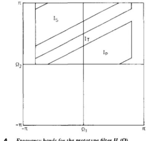
Let I , , I , , and I , be the passband, part of the tran- sition hand, and the stopband regions of H,(Cl), respec- tively, as shown in Fig. 4. The problem of designing a

2-D PFB of category A in the minimax sense is to design

H,(R) such that the peak ripples of T(R) - 1 and the stopband response of H,(Cl) are minimised simulta- neously. It can be formulated as follows:

minimise 6

subject to

I

H i @ )

+ H;(R

+

n)

- 1

1 <

6 for E I , U 1, for R E I , (14)

I

HO@) I

<

where ll = (0, n) and R is the ratio between the peak reconstruction error (PRE), i.e. the peak of

1

T(S1) - 1

1,

and the peak stopband resonse (PSR) of H,(R). Expr. 14 reveals that the corresponding design problem is a finite dimensional optimisation problem, but with an infinite number of nonlinear functional constraints. Instead of

6

Fig. 4 Frequenry handsfor the prototypefilter H0@)

(4)

solving this optimisation problem directly,

we

consider the problem of solving an approximation with a finite number of constraints for expr. 14. Let I , = {R,,,

a,,,

..., RpLl}, IT =

(%,

%-2, ..., QTJ, and 1s = {Qs,.

R,, , .

.

. , R,,,} be the sets of discrete frequency points uniformly distributed on I , , I T , and I , , respectively. By

evaluating the values of the nonlinear constraints of expr.

14 on the sets of discrete frequency points, the expression can be rewritten as follows:

minimise 6 subject to

I

Hg(R)

+

H;(R

+

n)

- 1

I

<

6 for R E I p U I ,

I

HdQ)

I

<

f o r R E I s (15)

Although expr. 15 contains a finite number of nonlinear functional constraints, it is not easy to solve. Next, we present a technique to solve the design problem based on a linearisation approach.

6

4 The proposed design technique 4.1 Linearisation of the nonlinear constraints Let a* = [a:, a:,

. . .

, a”,’ be the independent coefficient vector and H,,(R) be the corresponding magnitude response of the prototype analysis filter computed at the kth iteration during the optimisation process, where k denotes the iteration number and T the transpose oper- ation. Moreover, let AH,@) be the deviation in H,,(R)

corresponding to the perturbation Aa = [Aa,, Aaz,

. . .

,

Aa,], performed on ak. As a result, it follows from expr. 15 that we have minimise 6 subject to I(HOk(n)

+

AHO(n))2

+

( H O k ( a

+

n,

+

AH,(R

+

n))’

- 11

<

6 for R E Ip U I , Next, let

be the reconstruction error and the stopband response error of H,(R) computed at the kth iteration, respectively. Then, the constraint related to the reconstruction error shown in expr. 16 becomes

12H,,(Q) AH,(Q)

+

( A H o ( W

+

2HOk(Q

+

n)AH,(Q

+

n)

+

(AH,(R

+

n))’

- E:@)

I

<

6

for R E I p U I, (19) We assume that the solution of the independent coeffi-

cient vector a‘ is sufficiently close to the desired optimal solution of expr. 15. Then, the deviations AH@) and

AH,@

+

n)

corresponding to the optimal solution for I E E Proc.-Vis. Image Signal Process., Vol. 142, No. 4 , August 1995

expr. 16

are

expected to be close to

zero.

Therefore, the second order terms in expr. 19 can be neglected and expr.

16 becomes minimise 6 subject to

I2HodR) AH@)

+

2H,k(R

+ n)AH,(R

+

II)

- E)(R)

I

<

6

for R E I p U I ,

I R AH,(R) - E:@) I

<

6 for R E Is ₍₂₀₎ Based on expr. 20, we present an efficient method for solving the original design problem as shown in expr. 15 as follows.

4.2 An efficient method for solving expr. 15

First, we define several useful matrices and vectors. Let U , be an L , x M matrix with the (i. j)th element given by

upG,

j) = 2[Hok(Qpi)@,W,,)

+ HdQpi

+

n)@jtRFi

+ n)l

l < i < L , , l < j 5 M (21) Let U , be an L , x M matrix with the (i, j)th element given by

j) = 2[HOk(nTi)Qj(nTi)

+

H O k ( R T i

+

n)@ARTi

+

n)l

l < i < L , , l < j < M (22) Let Us be an L , x M matrix with the (i,j)th element given by

U&, j ) = R@,4Rsi) 1

<

i

<

L , , 1

<

j < M (23)

Let e, be an ( L ,

+

L,) x I vector given by e, =

[ W b , ) ,

w & 2 ) ,

. . .

, E:(R,,$

Et(nT2), , . ‘ I (24)

and let e, be an L , x 1 vector given by

e, =

[-Wsl),

. . .

,

E : ( ~ , , , ) l T

(25)

U = [ U : ,

a:,

U : ] ,

e = [e:, e:]’ (27)

Moreover, two additional matrices are defined as follows

(26)

Then, expr. 20 can be rewritten in the form of a dual

linear programming problem [20] as follows: maximise b’w

subject to A’w

<

c where

w = [Aa,, Aa,, ..., Aa,, 617

b = [OT, - 117 e = [eT, - - e T ] ,

(29)

(5)

[n eyn. 29, o is an M x I column vector with elements equal to zero and I , is an L x 1 column vector with elements equal to one, where L = L ,

+

L ,

+

L ,

.

Based on the dual affine scaling variant of Karmarkar's algorithm presented in [18], we introduce slack variables to the formulation of expr. 28. This leads to the following optimisation problem which is equivalent to expr. 28 ,

maximise b'w

subject to A'w

+

U = c U 2 0

where U is the 2L x 1 vector of slack variables. ible solution wo given by

From eqn. 29 we assume that we have an interior feas-

WO =

[

$ O ]

which satisfies ATw0

+

uo = c and uo > 0 at the initial stage. With the initial solutions wo and ,'U it has been shown in [21] that an appropriate scaling operation must be performed in order to update w and U such that the objective function b'w can be improved at a faster rate. In [IS] it was proposed to scale the slack variables as follows

0 = D,'u (31)

where D , = diag (U')

Substituting eqn. 31 into expr. 30, we obtain maximise b'w

subject to ATw

+

D,it = c

i t > O (33)

Let the set of the feasible solutions for expr. 28 be given by

W = { w E R'+' ~A'W

<

C } ₍₃₄₎

then the set of the feasible scaled slack vectors for expr. 33 is given by

P =

{ i t € R Z L 1 3 w ~ W , ATw

+

D u i = C } ₍₃₅₎

From expr. 35, it is easy to show that the corresponding

w in W for a given scaled slack vector it in P i s given by

4it)

= ( A D , l A T ) - L A D u - l ( D , l ~ - 6) (36) and the one-to-one relationship between the feasible directions h, in Wand ha in Pis given by

h; = -D;'ATh, (37)

Based on expr. 33 and eqn. 36, the feasible direction h, can be obtained by computing the gradient of the objec- tive function b'w with respect to it as follows:

(38) It then follows from eyn. 37 that the feasible direction h, is given by

h, = V;(bTw(6)) = - D , 1 A T ( A D , 2 A T ) - - ' b

h, = ( A D : A T ) - ' b (39) After determining h,, we consider the problem of finding a descent direction in order to update the independent 224

coefficient vector uk = [a:, a:,

...,

&IT

for expr. 15. Let the descent direction for ak be designated as d,,. From eqns. 29 and 39, we note that updating w can be carried out as follows:

w = wo

+

ah, =

[2O]

+ a[:]

if a suitable step size a is found. We use this da, which is the subvector containing the first M components of h,,

as an approximation of the true descent direction for the original optimisation problem in expr. 15. The next problem is to determine a suitable step size a for updating

d

during the optimisation process. Theoretically, the most suitable step size is obtained by employing a line search procedure to find the step size which minimises the following function:

f ( a ) = max max {

1

a )

+

B;(Q

+

II, a ) - t

I},

n E I p v I ,

max { R

I

W O ( Q a)

I}}

(40)

{

n E Is

where

fi,,@,

a ) and

R,(Q

+

II,

a) are the frequency responses of the prototype analysis filter with the updated filter coefficient vector a'

+

ad,. Doing this numerically would require a high degree of computational complexity. We propose an appropriate method by considering the feasibility of using the updated slack variable U'

+

ah,, to find the step size a analytically instead of numerically. First, from eqns. 31 and 37, we have the feasible direction for the unscaled slack variable as follows:

(41) Then, based on the fact that the updated slack vector U must be a vector with all elements greater than or equal to zero, a suitable step size a can be obtained by taking the maximum feasible step in the direction of h, as follows:

h, = - A T ( A D o - Z A T ) - l b = - A T h ,

a = min

{

- g l ( h J i < O}

where ( z ) ~ denotes the ith entry of the vector

z.

Although the step size a chosen by using expr. 42 is in general not the a which minimises expr. 40, our design experience shows that expr. 42 provides an efficient method for finding the step size for numerous designs.

From the above results, Algorithm 1 summarises the proposed design technique for solving the original design problem as shown in expr. 15 as follows:

Algorithm I

Step 1: Select a suitable initial guess for the coefficient vector a and set the iteration number k = 0.

Step 2: At the kth iteration, compute the frequency responses Hok(a) and Hok(R

+

I'I)

of the p-.totype analysis filter corresponding to the current filter coefficient vector U' and construct the matrix U and vector e using the results shown from eqn. 21-27. Then, set

wo = [0'6~]', where 6' = 1.001 max {

I

e

I

}.

Step 3: Find the slack vector uo = e -

A

'

W

'

=

[UT,

,]':U where u I = So/,

+

e, U, = 6'1, - e.

Step 4: Compute the feasible direction vector h, =

(AD;'AT)-'b for optimisation, where D , = diag (U). Instead of directly computing h, by performing the inverse of A D i 2 A T , we propose an efficient procedure as follows :

(6)

4.1

Construct

the diagonal matrices

D ,

= diag (U,)

4.2 Compute the diagonal matrix D = (0;'

+

0;'). 4.3 Compute the column vector x = U ( D ; *

4.4 Compute the value w = -(I;DI,)-'.

4.5 Solve the equation (UrDU

+

wxxT)d, = - w x

4.6 Compute the value h, = w(xrd,

+

1).

4.7 Form the desired direction vector hw = [d:h,lT. Step 5: Compute the feasible direction vector ho = - Arh, = [ h ~ , h ~ J T , where h,, = h, I , - Uda, hn2 =

Step 6 : Determine the step size a according to expr.

42. Then, update the coefficient vector U as follows:

$ + I =

d

+

ad,.

Step 7 : Define a performance indication function as

E(k) = max and D, = diag (u2).

- D,2)1,.

using Gaussian elimination to find d , .

ha I ,

+

Ud,.

roitows:

max

(1

H i @ )

+

H&(Q

+

n)

- 1

I),

n E l P v Ir

max { R

I

H d Q )

1))

(43)

{

r l s l s

It is reasonable to terminate the design process whenever the relative improvement to E(k) is small enough. There- fore, we stop the iterative procedure if

< K

E(k) - E(k

+

1)

4 4

where K is a preset small real number. Otherwise, set k = k

+

1 and go to Step 2.

5

To initiate the iteration when performing Algorithm 1 presented in Section 4, an initial guess for the coefficient vector a must be provided. Since the initial guess will affect the convergence speed and the design results, a good initial guess is usually one which is sufficiently close to the optimal solution of the considered problem. For the original design problem shown in expr. 15, we note that it is appropriate to use the optimal solution of the following least-squares design problem:

Selection of the required initial guess

minimise E,, =

₁

I

H;(Q)

+

H;(i2

+

n)

- 1

1'

n E I p " 1 r

+

R'

1

IHo(Q)12 (44)

R E I S

as the initial guess for Algorithm 1. Examining expr. 44, we note that it is just a 2-D extension of the 1-D least- squares Q M F design problem formulated in [19]. Hence, an algorithm for solving expr. 44 is developed based on the design method presented in [19] as follows:

Let a' be the filter coefficient vector of Ho(Q) com- puted at the ith iteration. Utilising the linearisation tech- nique of [t9], we reformulate expr. 44 as follows:

minimise

E,,

=

1

IHoi(Q)Ho(Q)

n e IF v I T

+

Ha@

+

rI)H,(R

+

n)

- 1

1'

(45) Following the matrices defined in eqns. 21-23, we con- struct the matrix

X

as follows:

x=+cu:

UT]' (46)

IEE Proc.-Vis. Image Signal Process., Vol. 142, N o . 4, August 1995

and rewrite the objective function

of

expr. 45 as follows:

E,, =(Xu -

z2)=(xu

- 1,)

+

(u,u)=(u,a) (47)

where I , denotes an ( L ,

+

L,) x t column vector with elements equal to one. Eqn. 47 reveales that E,, is a quadratic function of a. Therefore, the optimal U for expr.

45 can easily be found as follows:

(48) U =

( X X

+

U;

us)-

,(XTI*)

Using the optimal solution ofeqn. 48, we update the filter coefficient vector according to

u i f l = 0.5(ai

+

a ) ₍₄₉₎

Let

qi)

denote the value of E,, computed at the ith iteration. Again, it is reasonable to terminate the design process whenever the relative improvement to

qi)

is small enough. Therefore, we stop the iterative procedure if

Z(i) - E(i

+

1) E( i) <I?

where r7 is a preset small real number. After this process is terminated, the resulting filter coefficient vector is used as the required initial guess for Algorithm 1. However, the above approach for finding the required initial guess for Algorithm 1 is also an iterative process and hence an appropriate initial guess is also required. Our design experience shows that an appropriate method for selec- ting the initial guess for expr.

44

is to set it as follows:

a' =

(XF

X,

+

U: U,) - '(X,' 13) (51)

where

X,

is an L , x M matrix with its (i, j)th element given by

X d i , j ) =

@hQpi)

1 d i 6 L , , I

<

j d M (52) and

t3

is an L , x 1 vector with elements equal to one. Next, we summarise the algorithm which solves the optimisation problem of expr. 44 to provide the initial guess required by Algorithm 1.

Algorithm 2

Step I ; Compute the initial guess using eqn. 51 and set the iteration number i = 0.

Step 2: Compute the filter coefficient vector a using eqn. 48 at the ith iteration.

Step 3: Update the filter coefficient vector according to eqn. 49 to obtain a i + , .

Step 4 : Check if the stopping criterion given by expr.

50 is satisfied, then stop the design process. Otherwise, set i = i

+

1 and go to Step 2.

6 Simulation examples

We present a simulation example of designing 2-D PFBs using the proposed technique for illustration. This design is performed on a 80486 personal computer using MATLAB programming language. The values of K and r7 for terminating Algorithm 1 and Algorithm 2, respec- tively are both set to 0.001.

The design specifications used for this example are shown in Fig. 5. The 2-D PFB of category A has a lowpass prototype analysis filter of size 15 x 15. More- over, the maximum distance between any two adjacent grid points in the considered frequency bands is set to

n/32 and the ripple ratio R = 1 . By using the initial guess obtained from Algorithm 2, Algorithm 1 provides the design with some significant results after 22 iterations. These results include the PRE = 0.0169 dB of the 22s

(7)

designed 2-D P F B and the PSR = -54.19dB of the resulting analysis filter H 0 ( Q . The corresponding rnagni- tude responses of H,(Q), H , ( Q ) , and T(Q) are shown in Fig. 6.

-ll

-ll 0 1

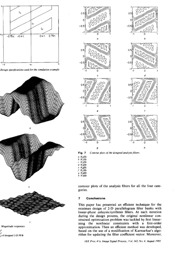
Fig. 5 Design speci3cations usedfor the simulation example

a

b

C

Fig. 6 Magnitude responses

226

The optimal analysis filter coefficients for each of the

2-D PFBs of categories B, C, and D can be obtained through a simple transformation of the filter coefficients designed for category A. Fig. 7 show the resulting

1 1 0 5 0 5 0 0 -0 5 -0 5 -1 1 1 0 0 1 a b 1 1 0 5 0 5 0 0 -0 5 -0 5 -1 1 0 1 0 1 C d 1 1 0 5 0 5 0 0 -0 5 -0 5 1 1 1 0 1 1 0 1 e f 1 0 5 0 -0 5 3 1 05 0 -0 5 - 3 1 -1 0 -1 0 1 9 h - 8

contour plots of the analysis filters for all the four categories.

7 Conclusions

This paper has presented an efficient technique for the minimax design of 2-D parallelogram filter banks with linear-phase anlaysis/synthesis filters. At each iteration during the design process, the original nonlinear constrained optirnisation problem was tackled by first linearising the nonlinear constraints with a first-order approximation. Then an efficient method was developed, based on the use of a modification of Karmarkar’s algorithm for updating the filter coefficient vector. Moreover, I E E Proc.-Vis. Image Signal Process.. Vol. 142, No. 4, August 1995

(8)

an analytical formula has been presented for calculating the step size required at each iteration. As a result, the

coefficients of the prototype analysis filters

can

be

obtained efficiently by solving only linear equations during the design process. An appropriate method for choosing the required initial guess has been presented in order to initiate the iterative design process. Computer simulations have shown that the proposed technique provides satisfactory design results.

8 References

I ESTEBAN, D., and GALAND, C.: ‘Application of quadrature mirror filler to split-band voice coding schemes’. Proc. IEEE 1977 Int. Conf. Acoust., Speech, Signal Processing, pp. 191-195 2 CROCHIERE. R.E.: ‘Digital signal processor: suhhand coding’, Bell

Syst.. Tech. J., 1981,60, pp. 1633-1653

3 BELLANGER, M.G., and DAGUET, J.L.: ‘TDM-FDM trans- multiplexer: digital polyphase and FFT‘, IEEE Trans. Commun.,

September 1974, COM-22, pp. 1199-1204

4 VETTERLI, M.: ‘Perfect transmultiplexers’. Proc. IEEE 1986 Int. Conf. Acoust., Speech, Signal Processing, pp. 2567-2570 5 VARY, P., and HEUTE, U,: ‘A short-time spectrum analyzer with

polyphase network and DFT”, Signal Processing, L980,2, pp. 55-65 6 HEUTE, U., and VARY, P.: ‘A digital filter hank with polyphase

network, and FFT hardware: measurements and applications’, Signal Processing, 1981 3, pp. 307-319

7 VETTERLI, M.: ‘Multidimensional subhand coding: some theory and algorithms’, Signal Processing. 1984.6, pp. 97-1 12

8 WOODS, J.W., and ONEIL, S.D.: ‘Suhband coding of images’, IEEE Trans. Acoust., Speech, Signal Processing, October 1986, ASSP-34, pp. 1278-1288

9 BAMBERGER, R.H., and SMITH, MJ.T.: ‘A filter bank for the directional decomposition of image: theory and design’, IEEE

Trans. Signal Processing, April 1992, ASSP-40, pp. 882-893

10 BAMBERGER, R.H., and SMITH, MJ.T.: ‘A multirate filter bank approach to the detection and enhancement of linear features in images’. Proc. 1991 IEEE Int. Conf. Acoust., Speech Signal Pro- cessing, pp. 2557-2560

11 TATHAM, R.H., KEENEY, J., and NOPON, I.: ’Application of the Tau-p transform (slant stack) in processing seismic reflection data’. Reprint of paper presented at 52nd Annu. Meeting SEC, Dallas, TX, 1982

I.? WACKERSREUTHER, G.: ‘On two-dimensional polyphase filter banks’, IEEE Trans. Acoust. Speech, Signal Processing, Feb. 1986, ASP-34, pp. 192-199

I3 VAIDYANATHAN, P.P.: hlultirate Systems and Filter Banks,

Prentice-Hall, Englewood Cliffs, NJ, 1992

14 KARLSSON, G., and VETTERLI, M.: ‘Theory of two-dimensional multirate filter banks’, IEEE Trans. Acoust., Speech, Signal Pro-

cessing, June 1990, ASP-38, pp. 925-937

15 CHEN, T., and VAIDYANATHAN, P.P.: ‘Recent developments in multidimensional multirate systems’, IEEE Trans. Circuits Syst. for

Video Technology, April 1993,3, pp, 116-137

16 VETTERLI, M., KOVACEVIC, J., and LEGALL, D.J. ‘Perfect reconstruction filter hanks for HDTV representation and coding’,

Signal Processing: Image Communication, October 1990, 2, pp. 349- 363

17 FORCHHEIMER, R., and KRONANDER, T.: ‘Image coding-from waveforms to animation’, I E E E Trans. Acoust., Speech, Signal Pro- cessing, December 1989, ASP-37, pp. 200&2023

18 ADLER, I., KARMARKAR, N., RESENDE, M.G.C., and VEIGA, G.: ‘An implementation of Karmarkar’s algorithm for linear programming’, Math. Programming, 1989,44, pp. 297-335

19 CHARNG-KANN CHEN, and JU-HONG LEE: ‘Design of quadrature mirror filters with linear phase in the frequency domain’, IEEE Trans. Circuits and Systems I f : Analog and Digital Signal Pro- cessing, September 1992,39, pp. 593-605

20 LUENBERGER, D.G.: Linear and Nonlinear Programming, MA: Addison-Wesley, 1984

21 HILLIER, F.S., and LIEBERMAN, G.J.: Introduction to Mathe- matical Programming, New York: McGraw-Hili, 1991