757
Acoustic and Shear-Wave Velocities in Hydrate-Bearing Sediments
Offshore Southwestern Taiwan: Tomography, Converted Waves
Analysis and Reverse-Time Migration of OBS Records
Philippe Schnürle1,*
, Char-Shine Liu1, and Chao-Shing Lee 2(Manuscript received 23 February 2006, in final form 4 December 2006)
ABSTRACT
1
Institute of Oceanography, National Taiwan University, Taipei, Taiwan, ROC
2
Institute of Applied Geosciences, National Taiwan Ocean University, Keelung, Taiwan, ROC
*
Corresponding author address: Dr. Philippe Schnürle, Institute of Oceanography, National Taiwan University, Taipei, Taiwan, ROC; E-mail: schnurle@oc.ntu.edu.twA 2.5-D combined seismic reflection and refraction survey has been conducted in the accretionary complex offshore of southwestern Taiwan where BSRs (Bottom Simulating Reflectors) are highly concentrated and geochemical signals for the presence of gas hydrate are strong. In this study, we perform velocity analysis of the 6 4-component OBS (Ocean-Bottom Seismometer) records along the southernmost transect of this seismic experiment. We utilize 3 independent methods in order to accurately de-termine the acoustic and shear-wave velocities of the sediments: 1-D Root Mean Square (RMS) analysis of the P-P and P-S reflected events on indi-vidual datumed components, 2-D inversion of the P-P and P-S reflected and refracted events along the in-line transect, and 3-D acoustic inversion of the first arrivals. The principal sources of bias in the determination of the velocities are the 3-dimentional nature of the topography and the com-plexity of the underlying structures. The three methods result in consistent velocity profiles. Rapid lateral and vertical variations of the velocities are observed. We then investigate the large scale gas hydrate content through rock physic modeling: at the vertical of each OBS, shear-waves velocities are utilized to estimate the water-filled porosities, and the acoustic veloci-ties predicted for a set of gas hydrate, quartz and clay contents are com-pared to the observed profiles.
(Key words: Ocean Bottom Seismometers, Acoustic and shear-wave velocities, Gas hydrates)
1. INTRODUCTION
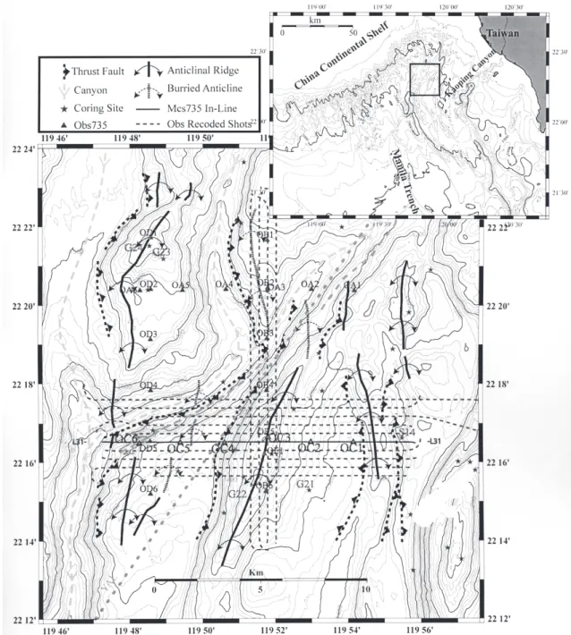
In the fall of 2004, a joint seismic reflection and wide-angle Ocean Bottom Seismometer (OBS) experiment was conducted offshore of southwestern Taiwan (Fig. 1), by the Institute of Oceanography, National Taiwan University and the Institute for Applied Geosciences, Na-tional Taiwan Ocean University. Hence, 6 OBSs (French IFREMER) were deployed for 4 hours recording time by the Ocean Researcher III vessel, while multi-channel seismic profil-ing was performed by the Ocean Researcher I vessel. The reflection seismic data is constituted by 42 east-west profiles with 400-m line spacing, about 14 km long and 9 north-south profiles about 16 km long. The 25-m spaced shots of small air-gun array, with a total volume of 580 in3, were recorded by a 24 channel solid streamer, 600 m in length (12.5-m group spacing) and the 4-component OBSs. A total of 4 OBS transects have been acquired. In this study, we analyze the east-west C transect located in the southern part of the dense seismic experiment. In addi-tion to the inline seismic profile MCS735-31, OBSC1 to 6 received the shots from up to 9 E-W off-line profiles, while OBSC3 also recorded 4 N-S cross-off-line profiles (Fig. 1); thus this OBS experiment is 2.5D.
In the survey area, a complex interplay between N-S trending thrust-bounded folds of the accretionary wedge and NE-SW oblique ramps, related to the Yung-An lineament are ob-served (Fig. 1). Drainage of the submarine Penghu Canyon is probably guided by this network of thrusts and strike-slip ramps. Fast accumulation of sediments derived from the Taiwan mountain belt deposit in the slope basins behind the anticlinal ridges. BSRs (Bottom Simulat-ing Reflectors) are widely observed in this region (Liu et al. 2006), with an average reflection coefficient of -0.094 (or 32% of the sea floor reflection value), and geochemical signals for the presence of gas hydrate are strong. Clear BSRs are observed almost continuously in the south-ern half of the survey box, while BSRs either appear as small patches or are absent in the northern half. Also, core samples collected in the study area consist essentially of mud, and present total organic carbon content (TOC) of about 0.5%, most often porosities of 60%, and bulk density from 1.6 to 2.2 g cm-3. High CH
4 concentrations in the bottom waters are found
at stations G23 (197 µL L-1), G22 (79 µL L-1), and N8 (613 µL L-1), and are probably of biogenic origin (-70 ~ -750
00 carbon isotopic ratio analyzed at sites N8 and N11; Chuang et al.
2006). Methane concentration in the core sediments at stations N6, N8, G15, G22, and G23 increases with depth, while rather randomly at other sites, with maximal values (in mL L-1) of 25 at G17, 21 at G21, 71 at G22, 133 at G23, 75 at N8 and 122 at N9 (Lin et al. 2006). Total sulfate depletion is generally observed through the bottom of the cores, and as shallow as 1 m beneath the sea-floor at site G23. Dissolved sulfide and high chloride concentrations are observed, but dissolved sulfide occurs before total sulfate depletion at several cores (Lin et al. 2006). Authigenic pyrites can be observed in the marine sediments where cold seeps of methane were found on the ocean floor, mostly as pyrite tubes porous in the center and the outer surfaces (Huang et al. 2006), and suggest long term gas seepage.
Laboratory measurements of pure structure I methane hydrate give density and acoustic velocity values ranging from 1.024 to 1.045 g cm-3 and 3.3 to 3.8 km s-1, respectively (Sloan 1998). Also, pure methane hydrate present a high shear-wave velocity of 1.89 km s-1 when compared to the typical low Vs of 100 - 600 m s-1 for deep marine hydrate-free sediments
Fig. 1. Structural setting and combined MCS/OBS seismic layout. The OBS
locations are marked by triangles. MCS735 shots recorded by the OBS transect C are marked with dashed lines, and the MCS735-31 in-line with a thick line.
(Waite et al. 2000). Further more, small quantities of gas bubbles in the pore space of marine sediments cause a dramatic decrease in compressional velocity (Domenico 1977), with little effect on the shear-wave velocity (Andreasen et al. 2003). Hence within hydrate/free gas-bearing sediments, the variations of compressional velocity, shear-wave velocity, and density with respect to the mineralogy, porosity and elastic coupling, have been investigated by nu-merous authors (e.g., Lee et al. 1996; Tinivella and Accaino 2000, Helgerud 2001; Chand et al. 2004). Thus, combined analyses of P-P and P-S multi-component records appears well suited for the characterization of gas-hydrate and free-gas bearing sediments (e.g., Mienert and Posewang 1999; Tinivella and Accaino 2000; Tréhu and Flueh 2001; Schnürle et al. 2004; Petersen et al. 2005). The aim of this paper is to investigate the means to retrieve accurately the acoustic and shear-wave velocities from the analysis of this OBS experiment and quantify the amount of gas hydrates at the OBS locations.
2. ACOUSTIC AND SHEAR-WAVE VELOCITY ANALYSES 2.1 Datuming and 1-D Root Mean-Square Velocity Analysis
Probably the most convenient approach to velocity analysis of OBS records consists in performing finite-difference datuming of the receiver gather to the OBS’s depth: Assuming no mode conversions occur at depth above the OBS (true for a flat sea-floor), the datuming pro-cess can be achieved by saving the time slices along a flat line of “receivers” at the depth of the OBS, during the acoustic reverse-time propagation of each of the 4 components. At such flat datum, conventional P-P root mean-square (RMS) velocity analysis tools can be utilized on the vertical and hydrophone components. Then, shear-wave RMS velocity scans are built on the horizontal components, using the acoustic velocity from the P-P analysis for the down-ward part. As the OBS spacing exceeds 2 km, common mid-point binning is not available, and RMS velocity analysis on the vertical and hydrophone components of our OBS datumed records has to be performed on the separate receiver gathers: the resulting acoustic velocities are thus considerably biased if the strata present significant dips. Conventional P-S depth binning is not feasible either, and shear-wave velocity analysis on the datumed horizontal components can only be performed with a priory conversion point’s location, fixed at 1/3 of the source-receiver offset in this study. Finally, the reverse time datuming can be extended to a full Re-verse-Time Migration (RTM) process, where the imaging times are provided by the acoustic or shear-wave travel-times from the OBS (Schnürle et al. 2005).
2.2 2-D Acoustic Wave Inversion
We then perform 2-dimentional inversion of the reflected, and refracted arrival of the inline shots of this OBS transect. The pre-processing sequence of the OBS records includes OBS relocation (see section 2.3) and geometry, band-pass filter, spiking-predictive deconvolution (the operator is mixed along 5 adjacent traces), time-offset variant gain, and a low-cut band-pass filter in order to enhance the reflected arrivals. The in-line multi-channel seismic profile MCS735-31, depth migrated with a constant 1480 m s-1 acoustic velocity above
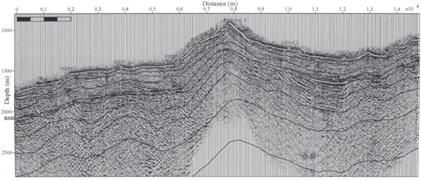
the sea-floor and a vertical velocity gradient of 0.79 m s-1 m-1 below, is used to generate the initial model: OBSs are relocated horizontally on the MCS735-31 profile and vertically to the sea-floor, and 9 layers are digitized (Fig. 2). Thus in addition to the sea-floor and BSR, we pick 2 reflectors within the sediments above the BSR, and 1 horizon below the BSR corresponding to reflection from the free gas zone and 3 additional horizons in the deeper part of the model.
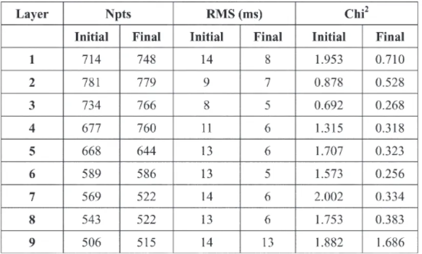
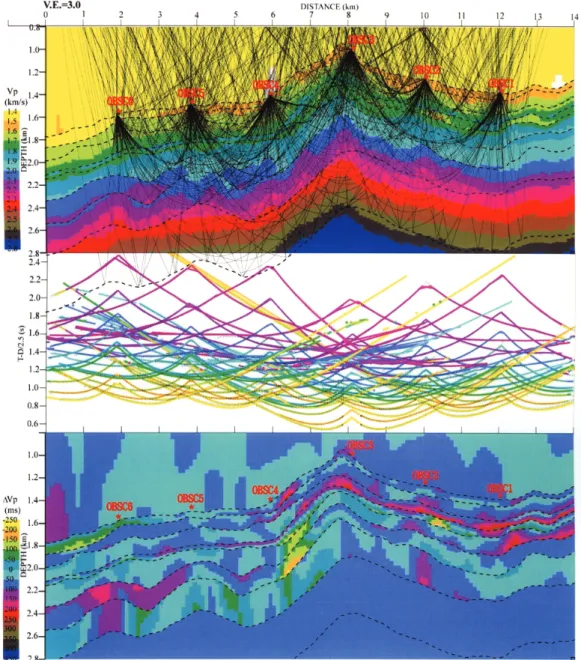
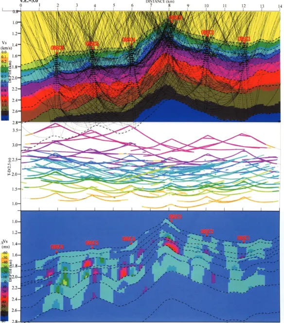
Ray tracing of acoustic as well as converted wave arrivals is performed with the 2-D RayInvr software, developed by Zelt and Smith (1992), with an input format modified from 10 to 1 m spatial definition and 1 m s-1 acoustic velocity accuracy. The velocity model is layer-based, with coordinal nodes extracted from the 9 digitized horizons and sampled every 100 m, and velocity nodes sampled every 400 m. For each OBS, we then performed ray tracing of the refracted acoustic waves and the reflections arising at the initial model’s interfaces. These modeled arrivals are then used to identify their observed time on the OBS records. A total of 6519 arrival-times are digitized. A damped least-square to the linearized inverse problem (Zelt and Smith 1992), using the partial derivatives of the travel times with respect to the model parameters and the travel time residuals is used to invert the acoustic velocities on the OBS transect. We perform 8 iteration in a layer-stripping approach: bottom velocities at the base of layer 1 to 4 (BSR), then at the bottom of layer 4 to 8 are inverted with a smooth damped least square, then top velocities in the next 2 inversion steps, and a second set of these 4 iterations is performed with a non-smoothed damped least-square procedure. The RMS travel-time misfit (in milliseconds)/normalized chi-square reduce from 12/1.483 to 7/0.511 (Table 1). Figure 3 shows the final velocity model, the ray paths, the observed and inverted travel-times, and the deviation from the initial model.
Fig. 2. Post-stack depth migrated section MCS735-31. A total of 9 horizons are
digitized for the node-based velocity model. OBS locations are indicated with crosses.
2.3 2-D Shear-Wave Inversion
The P-S mode converted reflections arising from our model’s interface are then used to invert the shewave velocities along the OBS transect. By comparing the predicted P-S ar-rivals and the horizontal components of our OBS data along a series of trial and error forward modeling, and using a layer striping approach, we are able to select average Poisson’s ratio for the 9 layers of our model (Table 2). Other modes of conversions, such as P-S downward transmitted then S-S reflected or P-P reflected then P-S upward transmitted waves are likely to present much smaller amplitudes (e.g., Schnürle and Hsiuan 2000) and are poorly identified on the horizontal components of our OBS data. Then, the P-P inverted acoustic velocities and the set of Poisson’s ratio are used to generate our initial shear-wave velocity model, observed P-S arrival times are digitized on the OBS records, and 4 iterations of the P-S travel-time inversion are performed. The RMS travel-time misfit (in milliseconds)/normalized chi-square reduce from 12/1.337 to 7/0.559 (Table 3). Figure 4 shows the final shear-wave velocities, a subset of the 19348 traced rays, the observed and modeled P-S arrival times, and the devia-tions of shear-wave velocities from the initial layer constant Poisson’s ratio model.
2.4 3-D First-Arrival Tomographic Inversion
FAST (First-Arrival Seismic Tomography), developed by Zelt and Barton (1998) appears well suited to performing a 3-dimentional inversion of the acoustic velocities from all the shots of this OBS experiment. The velocity model and the inverse grid are parameterized on a uniform square grid of 12 × 6 × 5.5 km (in in-line x, cross-line y, and depth z directions, respectively) with a 50 m node spacing. The forward calculation of travel-times and ray-paths
Table 1. Number of points, RMS travel-time residual and chi-squared during the P-P inversion. Larger misfits are observed for the direct arrivals (layer 1) and in the deepest layer.
Fig. 3. a) Subset of the 24721 rays and acoustic velocity model for the P-P
inversion. b) Modeled times are plotted with lines, observed times are marked with small bars representative of the 10 ms data incertitude. c) Deviation from the initial constant gradient model. OBS locations are indicated with stars.
Table 2. Poisson’s ratio, RMS travel-time residual and chi-squared during the P-S inversion.
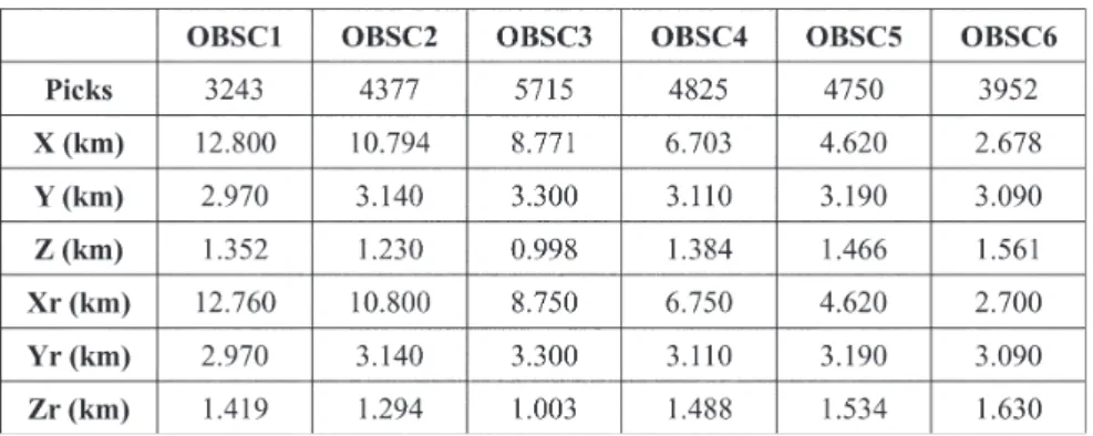
Table 3. Number of picked first-arrivals along in-line and cross-line, and OBS coordinates before and after relocation into the inversion grid.
uses the Vidale (1988, 1990) scheme modified to handle large velocity contrasts according to the method of Hole and Zelt (1995). A starting model and iterative approach is employed in which new ray paths are calculated at each iteration. The tomographic method is a regularized inversion incorporating a 25% smallest, and 75% vertical and horizontal flattest/smoothest perturbation constraint. The regularization is a jumping method in that the constraints are applied to the model perturbation with respect to the starting model. The sparse linear system of equations is solved using the LSQR variant of the conjugate gradient method described by Nolet (1987).
Fig. 4. a) Subset of the 24721 rays and shear-wave velocity model of the P-S
inversion. The up-going S ray paths are plotted with dashed lines. b) Modeled times are plotted with lines, observed times are marked with small bars representative of the 10 ms data incertitude. c) Deviation from the initial constant gradient model. OBS locations are indicated with stars.
A high-cut band-pass filter is applied in order to enhance the first arrivals the OBS dataset. Then, the first arrival times on the vertical and hydrophone component are digitized with a high-precision automatic picker, using cross-correlation and automatic snapping. A total of 26866 picks are used in the inversion. Each OBS is then relocated horizontally at the apex of the 3-D surface that best fits the water-wave arrivals, and vertically at the bathymetric depth of that relocation (Table 3). The starting model is built from the bathymetric data: the water velocity is constant at 1480 m s-1. Then, a vertical velocity gradient of 0.79 m s-1 m-1, chosen to best fit the first arrivals on the 6 OBS records, is applied below the bathymetric surface. Six iterations are performed and within each a maximum of 4 tradeoff parameters, that control the weighting of data misfit versus the constraint equations, are tested until the normalized misfit falls below 1, and the smallest/smooth/flattest model possible is selected. This model is then smoothed and input for the next non-linear iteration. The smoothing is necessary in order to spread the velocity updates across our model (particularly in the cross-line direction) and ap-pears critical in order to avoid that the rays concentrate in narrow zones. A 3 × 5 × 3 applied 3 times (in x, y, and z, respectively) during the first 3 iterations, and 2 × 4 × 2 applied 2 times during the 3 remaining iterations is used. The RMS travel-time misfit (in milliseconds)/nor-malized chi-square reduce from 258/66888 to 257/66164 after relocation, and down to 202/40743 through the inversion. Figure 5 shows a subset of the rays traced in the final model, the travel-times along these rays, and the observed travel-times with respect to offset. Figure 6 presents vertical and horizontal cross sections of the final velocity model and of the perturbations from the initial model.
3. DISCUSSION
3.1 1-D, 2-D, and 3-D Velocity Analysis Comparison
Our OBS survey allows us to perform 3 independent types of velocity analyses: 1-D RMS analysis of the P-P and P-S reflected events on individual datumed components (2 acoustic and 2 shear-wave records), 2-D inversions of the P-P and P-S reflected and refracted events along the in-line transect, and 3-D acoustic inversion of the first arrivals. Figure 7 presents true amplitude seismic depth images near each OBS, where one reverse-time migrated component is plotted over the MCS post-stack depth migrated section. Then, the 1-D, 2-D and 3-D de-rived acoustic and shear-wave velocities beneath each OBS are plotted next to the seismic image. When comparing the results from the three methods, several features can be outlined: a) Structural dips in the folds of the anticlinal ridges of the accretionary wedge (often exceed-ing 30 degrees) introduce an overestimation of the interval velocities in the 1-D P-P RMS analy-sis of the datum records. For instance, the velocity at the BSR beneath OBSC2 (Fig. 7b) or OBSC6 (Fig. 7f) of 2000 m s-1 reduces to 1735 m s-1, in good accordance with the 2-D and 3-D inversions, when accounting for the strata dip.
b) The shear-wave velocities retrieved from the 1-D P-S of the datumed horizontal records are equally biased by structural dips; however, the depth conversion of the 1-D RMS Vs profiles, performed with over-estimated Vp, stretches more than necessary the profile, resulting in
slower waves velocities at depth, as illustrated for OBSC6. Nevertheless, these shear-wave velocities are in good accordance (±150 m s-1) with those from the 2-D inversion. Each component leads to significantly different velocities, pointing out the uncertainty in-herent in the 1-D method. However better data preparation, in particular orientation and component separation, would improve these results. Also, the P-S semblance scans present rapid variations with depth that have not been included into this data analysis.
c) Although the 3-D relocation of the OBS slightly reduces the data misfit of the water-wave arrivals, relatively large variations of the velocities in the water column have to be assumed in order to fit our records (Fig. 6). Furthermore, in the 2-D inversion, the water column is
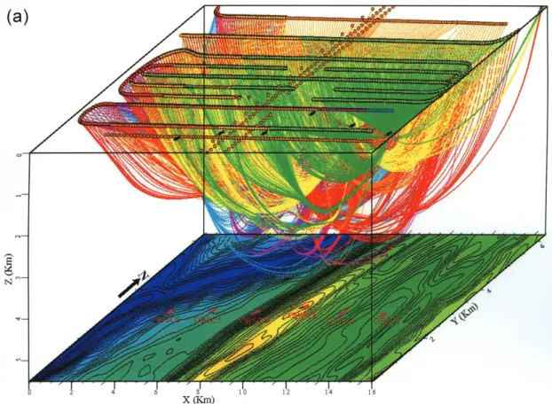
Fig. 5. a) 3D view from the southeast of the ray path during the first-arrival
tomo-graphic inversion. b) OBSC2 hydrophone record and first arrival (green). c) Travel-times along the rays (black circles) and observed (colored circles) in the final model. The data misfit for OBSC1 and 6, located at the extremities of our model, remains large.
Fig. 5. (Continued)
inverted as a single layer and presents ±50 m s-1 deviations from the initial 1480 m s-1 model (Fig. 3c), but the chi-squared of the sea-floor reflection during the P-P inversion remains larger than that of the remaining layers (except for the deepest layer 9 - Table 1): Future inversions will hopefully include several layers in the water column.
d) In the 2-D inversion, since the OBSs are spaced at 2.5 km, illuminations from adjacent OBS (data multiplicity) occurs only below layer 2 (Figs. 3a, b). Folding of the structures within layers 6 to 9 in the western-half of OBSC transect lead to triplications that degrade the velocity inversion.
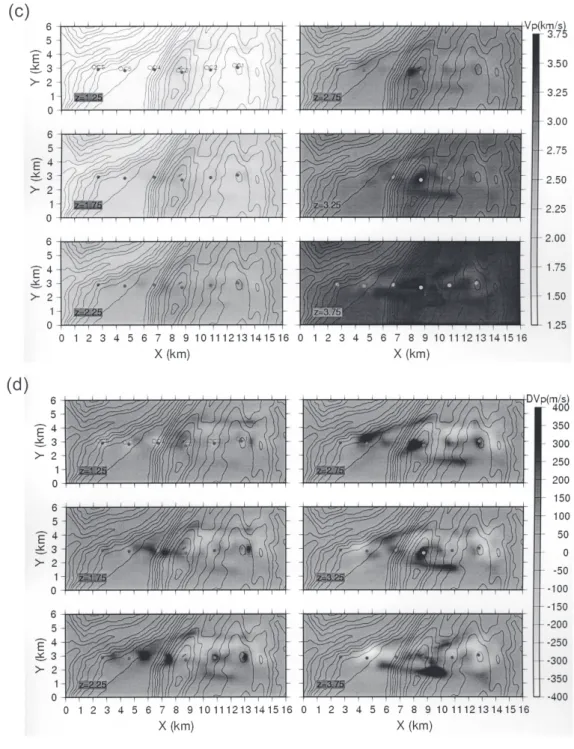
e) In the 3-D inversion, velocity features are well preserved laterally within a 2-km cross-line, as long as the ray coverage remains on a par. Rays coverage at depth greater than 3 km is limited to the center of the inversion grid, and deeper structures such as the top of the subducting south-China Sea oceanic basement are poorly resolved. The unreasonable
ve-Fig. 6. a) Vertical cross sections of the final acoustic velocity model between 1.5
and 4.0 km cross line. b) Vertical cross sections of deviation from the initial model. The sea-floor is marked by a thick line. OBS locations are indicated with circles on the y = 3 km section.
Fig. 6 (Continued). c) Horizontal cross sections of the final model between 1.25
and 3.75 km depth. d) Horizontal cross sections of the deviation from the initial model, plotted along rays. Bathymetric data is contoured at 50-m intervals. OBS locations are indicated with circles.
Fig. 7. Seismic depth images from component RTM migration of the OBS records
overlain on the MCS735 in-line depth migrated section, and acoustic and shear-waves velocities resulting from the 1-D RMS analysis of the 4 OBS datumed components (dashed lines), the 2-D RauInvr inversion, and the 3-D first arrival tomographic inversion (dash-doted lines). The seismic images have no vertical exaggeration. a) OBSC1-3 horizontal component. b) OBSC2-4 vertical component. c) OBSC3-1 hydrophone component. d) OBSC4-2 horizontal component. e) OBSC5-1 hydrophone component. f) OBSC6-2 horizontal component.
locity inversion that occurs at about 4 km in depth could result from the inclusion of the reflections (instead of refractions) arising from the plate interface into the 3-D inversion. f) The RTM depth images allow us to compare the events on each individual component and
the MCS reflection profile. The OBS migrated records are much less biased by out of plane reflection and structural complexity in general when compared to the MCS data. Furthermore, the largest acoustic velocity contrasts, particularly on OBSC1 to 4, correspond to the bright-est BSRs on the vertical and hydrophone components (Figs. 7b, c, and e). However, the base of the stability zone does not present large shear-wave velocity contrasts, nor generate strong P-S reflections on the migrated horizontal components (Figs. 7a, d, and f; e.g., Mienert and Posewang 1999).
3.2 Gas Hydrate Content
Several rock physics models have been proposed to predict the acoustic and shear-wave velocities of hydrate-bearing sediments; for instance, Chand et al. (2004) offer a review of models based on effective medium theory (e.g., Helgerud et al. 1999), while Guerin and Goldberg (2005) introduce grain-hydrate viscous friction and squirt flow mechanism, particu-larly suited for high frequency sonic waves logs. Models predict significantly different elastic properties, dependent on the interaction allowed between the sediments constituents and mi-cro-structure. Three principle models for gas-hydrate bearing sediments, involving the cemen-tation between grains, replacement of the matrix, and dissemination (“floating”) in the pore
Table 4. Elastic parameters utilized in the weighted equation model.
space have been proposed (e.g., Helgerud 2001). However in the absence of samples recov-ered at depth (drill holes), the principal difficulty remains to calibrate the elastic behavior of the hydrate-free sediments, i.e., the porosity and mineralogy (clay and sand contents in particular). In this study, the elastic properties of the sediments’ constituents are taken from Chand et al. (2004 - Table 4). We then explore the model space, varying the clay, quartz and hydrate contents, and test the fit between the velocities predicted and those retrieved from our data analysis, from the sea-floor to 1000 m sub-bottom depth. Thus, we first predict the water-filled porosity from the shear-wave velocities at the vertical of each OBS, then compute the resulting acoustic velocity and plot the residual with the acoustic velocities from our final model (Figs. 8a, b). We first use the 3-phase weighted equation (e.g., Lee et al. 1996): the acoustic and shear-wave velocities are computed with a weighted average of the Wood equa-tion (Wood 1941), best suited for hydrates floating in the pore-space, and the time-average equation (Wyllie et al. 1958), which is more appropriate for consolidated sediments. For this model, 0 and 25% clay and hydrate saturations lead to the most satisfactory results. Two consolidation factors for the clay-free (W = 1.5) and clay-rich (W = 2.0) sediments are se-lected to match the general velocity trends. A reasonable match is then obtained for hydrate-free sediments bellow the BSR, regardless of the clay content. Between the BSR and 200 m sub-bottom depth, hydrate saturations are accounted for by similar amounts in clay. Above a 200-m sub-bottom depth, the observed acoustic velocities are generally higher than those pre-dicted by the weighted equation, and no clay content or larger clay and hydrate content are necessary to produce a reasonable fit (Fig. 8a). We then follow the same procedure using the effective medium theory (Helgerud 2001; Lee and Collett 2001). For this model, the variations in predicted acoustic velocities increase considerably with increasing sub-bottom depth. Fur-ther more, large clay saturations are needed to match the general velocity trends. Above a 200-m sub-bottom depth, larger clay and hydrate content produce the best fit. Between 200 m and the BSR, about 60% clay and up to 25% hydrates are inferred. Finally, hydrate free sediments with more than 60% clay content between the BSR and a 600-m sub-bottom depth and less than 60% clay below 600 m produce a reasonable match in the deeper part of this model. Finally, the acoustic velocities present only minor evidence for the presence of free gas be-neath the BSR, and small velocity pull-down, extending laterally less than 1 km (Figs. 3, 7), are observed for OBSC2, OBSC3, and OBSC4.
Fig. 8a. Residual acoustic velocities (“observed” - modeled) as predicted from
the shear-wave and acoustic velocity profiles beneath OBSs from the weighted equation for hydrate and clay-free sediments (crosses), 25% hydrate (squares), 25% clay (stars), and 25% hydrate and clay (circles).
Fig. 8b. Residual acoustic velocities (“observed” - modeled) as predicted from
the shear-wave and acoustic velocity profiles beneath OBSs from the effective medium theory for hydrate and quartz-free sediments (crosses), 25% hydrate (squares), 60% clay (stars), and 25% hydrate and 60% clay (circles).
4. CONCLUSIONS
In this study, we have conducted 3 independent velocity analyses on 6 OBS records of a 2.5-D seismic experiment: 1-D RMS analysis of the P-P and P-S reflected events on individual datumed components, 2-D inversions of the P-P and P-S reflected and refracted events along the in-line transect, and 3-D acoustic inversion of the first arrivals. The 3 methods lead to similar velocity trends. The acoustic velocities inverted in this study present fairly localized deviations of
±200 m s-1 from our initial constant gradient 0.79 m s-1 m-1 model. Poisson’s ratios present a gradient of about 0.13 km-1 from the sea-floor down to the BSR. Minor shear-wave variations of ±30 m s-1 from the layer-constant Poisson’s ratio are observed. When considering acoustic and shear-waves velocity determination from a 1-D approach, the bias due to structural dips must be accounted for, either a-posteriori within the Dix law, or a-priori within a depth migra-tion process. The geometric bias in the cross-line direcmigra-tion remains uncompensated in the 2-D approach; first when projecting OBSs onto the inline transect, and second when building the layers from the MCS profile that is more prone to out of plane reflections than the OBS actu-ally is. Cross-line velocity variations as revealed from the 3-D inversion are a further source of uncertainty in the 2-D inversion. Finally, the acoustic and shear-wave velocities derived from the 2-D inversion are utilized to investigate large-scale gas hydrate content through rock phys-ics modeling. Given that little a-priori knowledge on the sediment properties at depth is available, we have difficulty distinguishing significant hydrate content from other mineralogies along this OBS transect. In future studies, we might therefore shift the focus to a vertical scale below that of velocity determination, i.e., a seismic wave-length of about 30 m, and make use of the amplitude and frequency content of the OBS records. Amplitude versus angle, within the pro-cess of a 3-dimentional reverse-time migration, shall be investigated.
Acknowledgments We would like to thank the Captains and crews of the R/V Ocean Re-searcher I and III for their efforts in collecting the combined MCS/OBS experiment used in this study. Long lasting discussions with Dr. W. B. Chen helped improving the first-arrival tomographic inversion. This study also benefited greatly from collaboration with CPC-EDRI and particularly with Dr. T. H. Hsiuan. Seismic Un*x (Center for Wave Phenomena, Colorado School of Mines; Stockwell 1999) is a wonderful platform for developing seismic processing tools (the RTM in this paper), and generating high quality seismic plots. Finally, we are grate-ful to Prof. T. K. Wang and an anonymous reviewer for their many constructive remarks. This study is supported by the Central Geological Survey grants 5226902000-06-93-01 and 5226902000-05-94-01.
REFERENCES
Andreassen, K., K. A. Berteussen, H. Sognnes, K. Henneberg, J. Langhammer, and J. Mienert, 2003: Multicomponent ocean bottom cable data in gas hydrate investigation offshore Norway. J. Geophys. Res., 108, 1-11.
Chand, S., T. A. Minshull, D. Gei, and J. M. Caricione, 2004: Elastic velocity models for gas-hydrate bearing sediments - a comparison. Geophys. J. Int., 158, 573-590.
Chuang, P. C., T. F. Yang, S. Lin, H. F. Lee, T. F. Lan, W. L. Hong, C. S. Liu, J. C. Chen, and Y. Wang, 2006: Extremely high methane concentration in bottom water and cored sediments from offshore southwestern Taiwan. Terr. Atmos. Ocean. Sci., 17, 903-920. Domenico, S. N., 1977: Elastic properties of unconsolidated porous sand reservoir. Geophysics,
42, 1339-1368.
Guerrin, G., and D. Golldberg, 2005: Modelling of acoustic wave dissipation in hydrate-beiring sediments. Geochem. Geophys. Geosyst., 6, 1-16.
Helgerud, M. B., J. Dvorkin, A. Nur, A. Sakai, and T. Collett, 1999: Elastic-wave velocity in marine sediments with gas hydrates: effective medium modeling. Geophys. Res. Lett., 26, 2021-2024.
Helgerud, M. B., 2001: Wave speed in gas hydrates and sediments containing gas hydrates: a laboratory and modeling study. Ph. D. Thesis, Stanf. Univ., USA, 248 pp.
Hole, J. A., and B. C. Zelt, 1995: Three-dimensional finite-difference reflection travel times.
Geophys. J. Int., 121, 427-434.
Huang, C. Y., C. W. Chien, M. Zhao, H. C. Li, and Y. Iizuka, 2006: Geological study of active cold seeps in the syn-collision accretionary prism Kaoping slope off SW Taiwan.
Terr. Atmos. Ocean. Sci., 17, 679-702.
Lee, M. W., D. R. Hutchinson, T. S. Collett, and W. Dillon, 1996: Seismic velocities for hydrate-bearing sediments from weighted equation. J. Geophys. Res., 101, 20347-20358. Lee, M. W., and T. S. Collett, 2001: Elastic properties of gas-hydrate-bearing sediments.
Geophysics, 66, 763-771.
Lin, S., W. C. Hsieh, Y. C. Lim, T. F. Yang, C. S. Liu, and Y. Wang, 2006: Methane migra-tion and its influence on sulfate reducmigra-tion in the Good Weather Ridge region, South China Sea continental margin sediments. Terr. Atmos. Ocean. Sci., 17, 883-902. Liu, C. S., P. Schnürle, Y. Wang, S. H. Chung, S. C. Chen, and T. H. Hsiuan, 2006:
Distribu-tion and characters of gas hydrate offshore of southwestern Taiwan. Terr. Atmos. Ocean.
Sci., 17, 615-644.
Mienert, J., and J. Posewang, 1999: Evidence of shallow and seep water gas hydrate destabili-zation in North Atlantic polar continental margin sediments, Geo-Mar. Lett., 19, 143-149. Nolet, G., 1987: Seismic wave propagation and seismic tomography. In: Nolet, G. (Ed.), in
Seismic Tomography, 23 pp.
Petersen, C. J., C. Papenberg, and D. Klaeschen, 2006: Local seismic quantification of gas hydrates and BSR characteristics from multi-frequency OBS data at the northern Hy-drate Ridge, in press.
Schnürle P., C. S. Liu, and C. S. Lee, 2005: Reverse-time migration of ocean bottom seis-mometer data. Annual Geophysics Meeting, conference proceedings, Nankang, Taiwan, 251-252.
Schnürle P., C. S. Liu, T. H. Hsiuan, and T. K. Wang, 2004: Characteristics of gas hydrate and free gas offshore southwestern Taiwan from a combined MCS/OBS data analysis. Mar.
Geophys. Res., 25, 157-180.
Schnürle P., and T. H. Hsiuan, 2000: Synthetic wide-angle seismic data in gas hydrate and free gas bearing sediments: a virtual OBS case study. Petrol. Geol. Taiwan, 34, 107-138. Sloan, E. D., 1998: Clatherates hydrates of natural gases. Marcel Decker, New York, 641 pp.
Stockwell, Jr. J. W., 1999: The CWP/SU: seismic Un*x Package, Computers and Geosciences, May 1999.
Tréhu, A. M., and E. R. Flueh, 2001: Estimating the thickness of the free gas zone beneath hydrate ridge, Oregon continental margin, from seismic velocities and attenuation. J.
Geophys. Res., 106, 2035-2045.
Tinavella, U., and F. Accaino, 2000: Compressional velocity and Poisson’s Ratio in marine sediments with gas hydrate and free gas by inversion of reflected and refracted seismic data (South Shetland Island, Antarctica). Mar. Geol., 164, 13-27.
Vidale, J. E., 1988: Finite-difference calculation of traveltimes. Bull. Seismol. Soc. Am., 78, 2062-2076.
Vidale, J. E., 1990: Finite-difference calculation of traveltimes in three dimensions. Geophysics, 55, 521-526.
Waite, W., M. B. Helgerud, A. Nur, J. C. Pinksto, L. Stern, and S. Kirby, 2000: Laboratory measurements of compressional and shear-wave speeds through methane hydrate. In: Holder, G. D., and P. R. Bishnoi (Eds.), Gas hydrate: challenges for the future, Ann. N. Y. Acad. Sci., New York, 1003-1010.
Wood, A. B., 1941: A text book of sound. Macmillian, New York, 578 pp.
Wyllie, M. R., A. R. J. Gregory, and G. H. F. Gardner, 1958: An experimental investigation of factors affecting elastic wave velocities in porous media. Geophysics, 23, 459-493. Zelt, C. A., and J. Barton, 1998: Three-dimensional seismic refraction tomography: a
com-parison of two methods applied to data from the Faeroe Basin. J. Geophys. Res., 103, 7187-7210.
Zelt, C. A., and R. B. Smith, 1992: Seismic travel time inversion for 2D crustal velocity structure. Geophys J. Int., 108, 16-34.
Schnürle, P., C. S. Liu, and C. S. Lee, 2006: Acoustic and shear-wave velocities in hydrate-bearing sediments offshore southwestern Taiwan: tomography, converted waves analysis and reverse-time migration of OBS records. Terr. Atmos. Ocean. Sci., 17, 757-779.