應用逆推網絡在克拉茲猜想的探討

(1)

國

立

交

通

大

學

應

用

數

學

系

碩

士

論

文

應用逆推網絡在克拉茲猜想的探討

Study 3n+1 problem in a backward iteration net

研究生 : 段

俊

旭

指導教授 : 張

書

銘博士

(2)

應用逆推網絡在克拉茲猜想的探討

Study 3n+1 problem in a backward iteration net

研究生 : 段俊旭

Student: Chun-Hsu Tuan

指導教授 : 張書銘博士

Advisor: Dr. Shu-Ming Chang

國立交通大學應用數學系

碩士論文

A Thesis

Submitted to Department of Applied Mathematics College of Science

National Chiao Tung University In Partial Fulfillment of the Requirements

for the Degree of Master

in

Applied Mathematics

May 2011

Hsinchu, Taiwan, Republic of China

(3)

應用逆推網絡在克拉茲猜想的探討

學生 : 段俊旭指導教授 : 張書銘博士

國立交通大學應用數學系 (研究所) 碩士班

摘要

本論文主要研究一個有名的數學問題 : 克拉茲猜想 (Collatz Conjecture)。雖然克拉茲猜想的形式與意義容易被理解，但它仍然尚未被證明。也因為如此，引發了我們對克拉茲猜想的興趣，也希望藉著研究對它有更多的了解。首先，我們會對克拉茲猜想做個簡單的介紹，並且整理一些其他人對克拉茲猜想做的研究。接下來，我們會建構一個特別的圖，也就是逆推網絡 (backward iteration net)，開始我們對克拉茲猜想的研究，同時我們也得到一些逆推網絡的特性。最後，我們嘗試建構一個模擬逆推網絡 (simulation backward iteration net)，去模擬實際的逆推網絡，根據兩者相互比較的數值結果做出分析結論。

關鍵詞 : 克拉茲猜想、逆推網絡、模擬逆推網絡。

(4)

Study 3n + 1 Problem in a Backward Iteration Net

Student: Chun-Hsu Tuan

Advisor: Dr. Shu-Ming Chang

Department (Institute) of Applied Mathematics

National Chiao Tung University

Abstract

3n+1 problem is one of the most famous conjectures in mathematics. It can be easily

understood even younger children who just know how to divide by 2 and multiply by 3. However, the 3n + 1 problem still can not be proved yet. Therefore, we are so interested in this problem and hope to understand it completely. First, our study gives a brief introduction of the 3n + 1 problem, and we list some results in many research of the 3n + 1 problem. Then, we use a graph, a backward iteration net, to examine the 3n + 1 problem and obtain some properties in the backward iteration net. Finally, we simulate the backward iteration net and compare the numerical results with the net.

(5)

誌謝

本篇論文的完成，最要感謝的就是我的指導教授張書銘老師，老師不僅是在研究上給我許多指導與方向，也教導我許多做人處事的道理與態度，在我遇到瓶頸的時候，老師總是不厭其煩的開導我鼓勵我，在我太過得意的時候，老師也會適時提醒該注意的小細節，在研究所生涯，受到老師的照顧與幫助實在是太多了老師，謝謝你帶給我的一切，真的非常謝謝老師。同時也要感謝我的口試委員楊一帆老師和何南國老師，謝謝你們給我許多指導，也提供了許多可以嘗試的方向與改進的方法，非常謝謝老師們。在做研究與求學期間，我也要感謝所有修過課的老師們，謝謝你們教給我的許多概念與不同的知識領域，讓我有足夠的背景知識，讓這篇論文能夠有較為完整的呈現，在此特別謝謝老師們的教導。接下來，我要特別感謝媽媽、姑姑、叔叔、陳秋媛老師、吳慶堂老師、加鹽、耀宗、謝慶勳、貓達、小太、美女、GG 王、小 p、小吵、小泡、文昱、林志嘉、蜘蛛、劉崙欣、Blue，以及同師門的暉哥、林育賢、大鋼、定國、吳啟豪、黃柏綸、許尚。在論文難產的時候，多虧有你們的陪伴鼓勵開導，得到許多你們的溫暖與協助，最終這篇論文才得以順利誕生，在此獻上誠摯的感謝，也把這份榮耀與你們分享。三年的研究所生涯，親身體悟了許多酸甜苦辣，人生中最好與最差的狀態在這期間也一併經歷。幸運的是，老師跟最親愛的家人朋友總是在我身邊，給我許多關懷與包容，讓我有足夠勇氣繼續往前走，希望我能好好記得這些深刻的種種在未來把它們都化為正面力量，為自己創造一個美好的人生，不讓自己與所有關心我的人們失望，並期許自己未來有能力當一個小太陽，帶給你們許多溫暖與歡樂。最後，我想把這份成果獻給我最摯愛的爸爸。爸，我知道你一直在我身邊保佑著我，謝謝你，未來我也會好好努力不讓你失望，當一個讓你感到驕傲的兒子。爸，希望這份喜悅與榮耀你也能與我一同分享。段俊旭謹誌于交通大學 2011 年 5 月 iii

(6)

List of Figures

1 β4(10) . . . 8

2 The partial framework of βk(1). . . 9

3 The number relation in the 3n + 1 backward iteration net. . . . 12

4 The number relation in the 3n + 1 backward iteration net. . . . 12

(8)

1 Introduction

What’s the 3n + 1 problem? The 3n + 1 problem can be presented by many ways. Attributed to L. Collatz, he deﬁnes the Collatz function as

C(n) =    3n + 1, if n is odd. n 2, if n is even.

The 3n + 1 problem states that for each n∈ N, there is a k ∈ N, such that C(k)(n) = 1, that is, any natural number will eventually iterate to 1 in ﬁnite iterations.

1.1 History of 3n + 1 Problem

The 3n + 1 problem is not only famous but historical. The 3n + 1 problem is presented about in the 1950s. It is often called “Syracuse conjecture”. It is said that the 3n + 1 problem is ﬁrst researched in American Syracuse University. [1]

For the same time, many mathematicians are interested in the 3n + 1 problem in the middle of the 20th century. American mathematics master, Martin Gardner, who called the 3n + 1 problem “Hail conjecture”. Why did he call it? Because the 3n + 1 problem has a special phenomenon, sometimes the numbers will go larger but sometimes will go smaller. It’s like that the hail inﬂuenced by air, it sometimes goes up and sometimes goes down between cloud layers in summer. Hence, it is called “Hail conjecture”.

Afterward, Japanese scientist, Shizuo Katutani, brought the 3n + 1 problem from Europe to Japan, and he got some results: the 3n + 1 problem doesn’t hold for negative integers. Thus the 3n + 1 problem is also called “Katutani conjecture”. In 1996, Thwaites oﬀered 1100 pounds for its solution, so the 3n + 1 problem had another name “Thwaites conjecture”. [1]

Besides, the 3n + 1 problem has many kinds of names: Collatz conjecture, Hasse problem, Ulam problem. They are all about the mathematicians or places in researching the 3n + 1 problem. For the reason, the 3n + 1 problem has unique charisma in mathematics. [1]

Owing to the rapid develop of computer science in the 20th century’ end, scientists use computers mighty computing speed to solve the 3n + 1 problem. Until now, about the natural numbers veriﬁcation on 3n + 1 problem, from 1 to 20× 258 ∼ 5.764 × 1018 [6], among these natural numbers, they all eventually will iterate to 1, and enter 1− 4 − 2 − 1 cycle. That is, they all hold for the 3n + 1 problem.

However, no matter computers can check how large natural numbers for the 3n+1 problem, it still can’t be proved by this way. How to solve the 3n + 1 problem is what we continue to

(9)

strive.

1.2 Some Definitions and Results for The 3n + 1 Problem

For a long time, many mathematicians try kinds of ways to analysis 3n+1 problem. Although 3n + 1 problem is still an open problem, they get some results about it. In this subsection, we will introduce some deﬁnitions, records, and results about their research for 3n+1 problem.

Definition 1.1 ([16]). Let f (n) := n/2, if n is even, and f (n) := 3n+1, if n is odd. Choosing

a natural number x as staring number and applying f repeatedly produces a sequence of natural numbers, which is called f − trajectory of x and denoted by

Γf(x) := (x, f (x), f (f (x)), . . . , fk(x), . . .).

For example, taking x = 13 gives the f-trajectory, then

Γf(13) = (13, 40, 20, 10, 5, 16, 8, 4, 2, 1, 4, 2, 1, ...) which continues periodically with the cycle

(4, 2, 1). There are many starting numbers which have been tested. This leads to the 3n + 1 problem which asserts that any f-trajectory eventually runs into the limiting cycle (4,2,1).

In 2002, David Gluck and Brian D. Taylor had some results about the statistic of ﬁnite Collatz trajectory. The Theorem 1.2 gives more precise description.

Theorem 1.2 ([8, 11]). If a = (a1, a2, . . . , an) is a ﬁnite Collatz trajectory starting from a1,

with an = 1 being the ﬁrst time 1 is reached and the statistic

C(a) = a1a2+ a2a3 +· · · + an−1an+ ana1

(a1)2+ (a2)2+· · · + (an)2

. Then ₁₃9 ≤ C(a) ≤ 5₇.

In the following, we will introduce the function T . In 3n + 1 problem research, several authors prefer to deal with T instead of f .

Definition 1.3 ([4, 11, 16]). Let map T :N → N given by

T (x) =    3x+1 2 if x≡ 1 (mod 2). x 2 if x≡ 0 (mod 2).

(10)

This function T replaces the function f deﬁned above without loss of information: if n is even, then T (n) = f (n), and if n is odd, then T (n) = f (f (n)) (as 3n + 1 is even whenever n is odd). In this sense, T “shortens” the f-trajectories. Similar to f-trajectory, the T-trajectory of an integer n is the set

O+(m) := (m, T (m), T (T (m)), . . . , Tk(m), . . .).

The structure of the positive integers forces any orbit of T to iterate to one of the following: (1) the trivial cycle (1,2);

(2) a non-trivial cycle;

(3) inﬁnity (the orbit is divergent).

The 3n + 1 problem claims that option (1) occurs in all cases. That is, the 3n + 1 conjecture asserts that for any starting number in N, the T-trajectory eventually ends in the cycle (1,2). Moreover, there is a T-trajectory conjecture as follows:

No divergent trajectory conjecture.[16] There is no divergent 3n + 1 trajectory, i.e., there

is no y∈ N such that lim

n→∞ T

(n)_{(y) =}_∞.

Definition 1.4 ([4, 11, 16]). The stopping time σ(n) of n is deﬁned by

σ(n) = inf{k : fk(n) < n}.

Why do we interested in σ(n)? If any σ(n) is ﬁnite, then the 3n + 1 conjecture holds. Why? First, check that every positive integer up to N − 1 iterates to 1, then consider the iterates of N . Once the iterates go below N , you are done. For this reason, one considers the so-called stopping time of n.

Definition 1.5 ([4, 11, 16]). The total stopping time σ_∞(n) of n is deﬁned by

σ_∞(n) = inf{k : fk(n) = 1}. The 3n + 1 conjecture holds if any σ_∞(n) is ﬁnite.

Definition 1.6 ([4, 11, 16]). The height h(n) of n is deﬁned by

(11)

In [1], the author uses a interesting description to introduce σ(n), σ_∞(n), h(n). The author calls “the nth flight” as the starting value n, “keeping height distance” as σ(n), “flight distance” as σ_∞(n), and “maximum flight height” as h(n). For example, the 11st flight is

11→ 34 → 17 → 52 → 26 → 13 → 40 → 20 → 10 → 5 → 16 → 8 → 4 → 2 → 1. By observing the 11st flight, we know the maximum flight height is 52, h(11). Moreover, the flight distance is 14, σ_∞(11). Specially, the keeping height distance is 7, σ(11). The author defines the flight distance of the 1st flight is 0. In the following, from n = 1 to n = 30, the author list σ(n), σ∞(n), h(n) as follows:

n 1 2 3 4 5 6 7 8 9 10 11 12 13 14 15 σ_∞(n) 0 1 7 2 5 8 16 3 19 6 14 9 9 17 17 σ(n) 0 0 5 0 2 0 10 0 2 0 7 0 2 0 10 h(n) 1 2 16 4 16 16 52 8 52 16 52 16 40 52 160 n 16 17 18 19 20 21 22 23 24 25 26 27 28 29 30 σ_∞(n) 4 12 20 20 7 7 15 15 10 23 10 111 18 18 18 σ(n) 0 2 0 5 0 2 0 7 0 2 0 95 0 2 0 h(n) 16 52 52 88 20 64 52 160 24 88 40 9232 52 88 160

However, based on [16], L. E. Garner(1984) deﬁned the height of a natural number n the least non-negative integer k such that Tk _{= 1 (if such k exists). That is,}

hT(n) := min{k ∈ N ∪ {0} : Tk(n) = 1}

L. E. Garner proved the theorem as follows:

Theorem 1.7 ([7]). There are inﬁnitely many pairs of consecutive positive integers (n, n + 1)

whose T-trajectories coincide at a certain step, i.e. there is a non-negative integer k with the property Tk_{(n) = T}k_{(n + 1).}

About “consecutive integer pairs of the same height in the Collatz conjecture”, Wu Jia Bang and Huang Guo Lin [17] have investigated pairs of successive integers of the same hight. They found that families of consecutive integer pairs of the same height occur inﬁnitely often and in diﬀerent patterns.

Remark 1.8 ([1]). On Collatz function, the author calls f (n) = n/2 “even transformation”,

(12)

n iterating to 1 process, the author counts the total number of odd transformation, denoted O(n), and counts the total number of even transformation, denoted E(n). Thus, σ_∞(n) =

O(n) + E(n).

Based on [1], the relation between O(n) and E(n) was proved as the following theorem:

Theorem 1.9. For any n∈ N, O(n)/E(n) < log 2/ log 3.

Definition 1.10 ([4, 16]). For a∈ Z+_{, the predecessor set of a is deﬁned by}

PT(a) := {b ∈ Z+: T(k)(b) = a for some k∈ Z+}.

In brief, PT(a) is set of numbers which approach a given number a on T-function. Thus,

by the deﬁnition, we realize that the 3n + 1 conjecture holds if PT(1) ≡ N.

Definition 1.11 ([4, 16]). For a ∈ Z+_{, the counting function of predecessor set of a not}

exceeding a given bound x is deﬁned by

Za(x) := |{n ∈ PT(a) : n≤ x}|.

By the deﬁnition of Za(x), we realize that the 3n + 1 conjecture holds if Z1(x) = x for all

x≥ 1. The size of Za(x) was ﬁrst studied by Crandall, who proved the theorem below:

Theorem 1.12 ([5]). There is a positive constant c such that Z1(x) > xc for suﬃciently large

x∈ N.

Based on [5, 16], Wirsching [15](1998) notes that this result extends to Za(x) for all a̸= 0

(mod 3). Using the tree-search method of Crandall, Sander [13](1990) gave a speciﬁc lower bound, c = 0.25. This ”tree-search method” has been improved by D. Applegate and J. C. Lagarias [2](1995), arriving at a computer-assisted proof for c = 0.654. Using functional diﬀer-ence inequalities, Krasikov [9](1989) succeeded in proving Za(x) > xc with c = 3/7 ≈ 0.42857,

for suﬃciently large x and certain numbers a ∈ N (including a = 1). Wirsching [14](1993) used the same approach to obtain c = 0.48. Applegate and Lagarias [3](1995) superseded these results with Z1(x) > x0.81, for suﬃciently large x, by enhancing Krasikov’s approach

with nonlinear programming. Recently, Krasikov and Lagarias [10](2002) streamlined this approach to obtain

Z1(x) > x0.84, x suﬃciently large.

On the other hand, there are some results about computational veriﬁcation of 3n + 1 conjecture. Based on [6], in 1996, the team of Tomas Oliveira e Silva wrote a computer

(13)

program to test the 3n + 1 conjecture. In 1999, they reported on computations verifying the 3x + 1 conjecture for n < 3× 253≈ 2.702× 1016. In 2004, they devised an improved algorithm to test the 3n + 1 conjecture, about three times faster than their previous one. Thus, they restarted the verification efforts in 2004, however, they stopped the work in January 2009. Nevertheless, they have verified the 3n + 1 conjecture up to

20× 258= 5764607523034234880 > 5.764× 1018.

Besides, the team of Eric Roodendaal [12] maintains an ongoing distributed search program for verifying the 3n + 1 conjecture to new records. As of February 2008 the 3n + 1 conjecture is veriﬁed up to 612× 250 _{≈ 6.89 × 10}17_{. The current record happens in February 2011, they}

have veriﬁed the 3n + 1 conjecture up to

964× 250≈ 1.805 × 1018.

In the following, about the deﬁnitions mentioned above, we classify the equivalent propo-sitions of 3n + 1 problem in Remark 1.13.

Remark 1.13. If the 3n + 1 problem holds, then it is equivalent to the following propositions:

(1) For any starting value n ∈ N, the f-trajectory Γf(n) eventually runs into the limiting

cycle (4,2,1).

(2) For any starting value n∈ N, the T-trajectory O+(n) eventually runs into the limiting

cycle (2,1).

(3) For any starting value n∈ N, the stopping time σ(n) is ﬁnite.

(4) For any starting value n∈ N, the total stopping time σ_∞(n) is ﬁnite.

(5) For predecessor set of 1, PT(1) ≡ N.

(6) For all x≥ 1, Z1(x) = x.

In this section, we have preliminary concepts about the 3n + 1 problem. In the following, we will introduce the 3n + 1 backward iteration net, which is an important role in our study in the 3n + 1 problem.

(14)

2 The 3n + 1 Backward Iteration Net β

_k

(n)

What’s the 3n+1 backward iteration net ? A 3n + 1 backward iteration net is constructed by a starting value n∈ N and the formula of 3n + 1 backward iteration. Why are we interested in the 3n + 1 backward iteration net? In the beginning, our idea about the 3n + 1 problem is: if any natural number will iterate to 1 in ﬁnite transformations on Collatz function, then, in other words, if we start from 1 and apply the 3n + 1 backward iteration formula, can we strength all the natural numbers set? If we can, then we equally solve the 3n + 1 problem. Therefore, the 3n + 1 backward iteration net is the chief topic what we strive. In this section, we will introduce the 3n + 1 backward iteration formula I, the 3n + 1 backward iteration net

βk(n), and relation between natural numbers in βk(n), and some properties of βk(n).

2.1 Formula

In this subsection, we will introduce the formula of 3n+1 backward iteration. In fact, the 3n + 1 backward iteration is the inverse operator of Collatz function, denoted by I on the domainZ+_{, its formula is below:}

I(n) =    {2n}, n ∈ N \ {6k + 4|k ∈ N ∪ {0}}. {2n, (n − 1)/3}, n ∈ {6k + 4|k ∈ N ∪ {0}}.

We deﬁne I(0)_{(n) = n, I}(k)_{(n) =}_{{q|q ∈ I(p), p ∈ I}(k−1)_(n)_{}, k ∈ N. In the following, we will}

apply I to construct the 3n + 1 backward iteration net.

2.2 The 3n + 1 Backward Iteration net β

k

(n)

In this subsection, we will introduce how we apply I to construct the 3n+1 backward iteration net. We deﬁne βk(n) as a 3n + 1 backward iteration net constructed by a starting value n∈ N

and iterating k times on I, k∈ N. Moreover, βk(n) is a directed graph consisting of the vertex

set V (βk(n)) and the E(βk(n)). In the following, we will introduce the deﬁnition of directed

graph and deﬁne the corresponding notations for βk(n).

Definition 2.1. A directed graph or digraph G is a triple consisting of a vertex set V (G), an

edge set E(G), and a function assigning each edge and ordered pair of vertices. In a digraph, we write (u,v) for an edge. If there is an edge from u to v, then v is a successor of u, and u is a predecessor of v. We also write u→ v for ”there is an edge from u to v”.

(15)

By use of Deﬁnition 2.1, we give a more precise deﬁnition of the 3n + 1 backward iteration

βk(n) as follows:

Definition 2.2. In a 3n + 1 backward iteration net βk(n), the deﬁnitions of V (βk(n)),

E(βk(n)), and the edge (p,g) for βk(n) as follows:

1. V (βk(n))={p|p ∈ {n}

∪

I(1)_(n)∪_I(2)_(n)∪_{· · ·}∪_I(k)_(n)_}.

2. E(βk(n))={(p, q)|p, q ∈ V (βk(n)) and q ∈ I(p)}.

3. We denote an ordered pair (p,q) for an edge, if q ∈ I(p), p, q ∈ V (βk(n)). We also write

p→ q for “there is an edge from p to q”.

For convenience, we let I(k)_{(n) be L}

k, called level k. In the following, we take β4(10) as

an example to explain.

(16)

By observing Figure 1, we can easily realize that β4(10) is constructed by the starting

value 10 and iterating 4 times on I. Then, we will explain the vertex set V (β4(10)) and the

edge set E(β4(10)) as follows:

1. Since L0 = I(0)(10) = 10, L1 = I(1)(10) = {3, 20}, L2 = I(2)(10) = {6, 40}, L3 =

I(3)_{(10) =}_{{12, 13, 80}, L}

4 = I(4)(10) ={24, 26, 160}. Hence, the vertex set V (β4(10)) =

{10, 3, 20, 6, 40, 12, 13, 80, 24, 26, 160}.

2. Since V (β4(10)) = {10, 3, 20, 6, 40, 12, 13, 80, 24, 26, 160}, and I(10) = {3, 20}, I(3) =

{6}, I(20) = {40}, I(6) = {12}, I(40) = {13, 80}, I(12) = {24}, I(13) = {26}, I(80) = 160. Hence, the edge set E(β4(10)) = {(10,3), (10,20), (3,6), (20,40), (6,12),

(40,13), (40,80), (12,24), (13,26), (80,160)}.

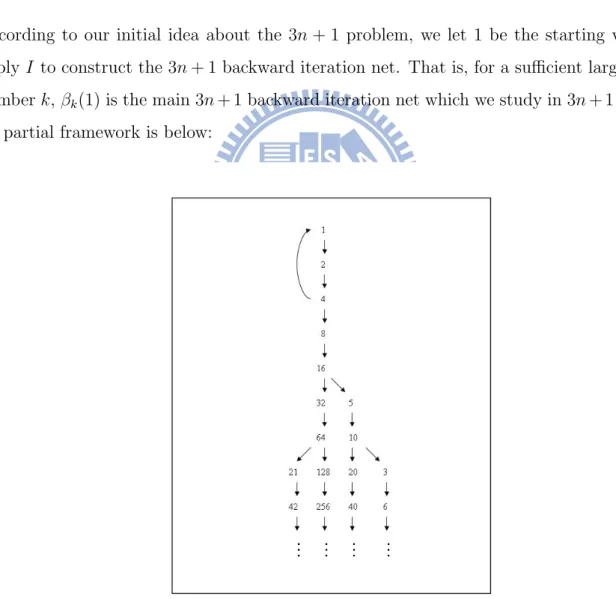
According to our initial idea about the 3n + 1 problem, we let 1 be the starting value and apply I to construct the 3n + 1 backward iteration net. That is, for a suﬃcient large natural number k, βk(1) is the main 3n + 1 backward iteration net which we study in 3n + 1 problem.

Its partial framework is below:

(17)

In order to know the 3n + 1 backward iteration net more, in the following, we will intro-duce the relation between natural numbers in the 3n + 1 backward iteration net.

2.3 The Relations Between Natural Numbers Under One

Trans-formation On I

By observing the 3n + 1 backward iteration net, we realize that one natural number may backward iterate to another two diﬀerent natural numbers. In this subsection, we partition the natural numbers set into six parts to realize the relations between natural numbers under

one transformation on I in the 3n + 1 backward iteration net. In this way, we also can clearly

realize that the “edges” are “from whom to whom” in the 3n + 1 backward iteration net. The six partitions of natural numbers set which we classify as follows:

A :={6k + 1|k ∈ N ∪ {0}}; B :={6k + 2|k ∈ N ∪ {0}}; C :={6k + 3|k ∈ N ∪ {0}}; D :={6k + 4|k ∈ N ∪ {0}}; E :={6k + 5|k ∈ N ∪ {0}}; F :={6k + 6|k ∈ N ∪ {0}}.

For consistence, we let a ∈ A, b ∈ B, c ∈ C, d ∈ D, e ∈ E, f ∈ F. In the following, we will classify the relations between the natural numbers under one transformation on I in 3n + 1 backward iteration net.

(1) For a∈ A, ∃b ∈ B s.t. I(a) = {b}, that is, a → b.

It shows that a must backward iterate to b under one transformation on I. Since a = 6k + 1 for some k ∈ N ∪ {0} , then I(a) = {2(6k + 1)} = {12k + 2} = {6(2k) + 2}. That is, there exists b = 6(2k) + 2∈ B s.t. I(a) = {b}.

(2) For b∈ B, ∃d ∈ D s.t. I(b) = {d}, that is, b → d.

It shows that b must backward iterate to d under one transformation on I. Since b = 6k + 2 for some k ∈ N ∪ {0} , then I(b) = {2(6k + 2)} = {12k + 4} = {6(2k) + 4}. That is, there exists d = 6(2k) + 4∈ D s.t. I(b) = {d}.

(18)

(3) For c∈ C, ∃f ∈ F s.t. I(c) = {f}, that is, c → f.

It shows that c must backward iterate to f under one transformation on I. Since c = 6k + 3 for some k ∈ N ∪ {0} , then I(c) = {2(6k + 3)} = {12k + 6} = {6(2k) + 6}. That is, there exists f = 6(2k) + 6∈ F s.t. I(c) = {f}.

(4) For d∈ D: d → {b, a}, or d → {b, c}, or d → {b, e}.

It shows that d may backward iterate to {b, a} , {b, c} , or {b, e} under one transformation on

I.

proof : Specially, d will backward iterate to another two diﬀerent natural numbers. Since d = 6k + 4 for some k∈ N∪{0}, one is I(d) = {2(6k +4)} = {12k +8} = {6(2k +1)+2}, that

is, there exists b = 6(2k+1)+2∈ B s.t. I(d) = {b}. And another is I(d) = {((6k+4)−1)/3} =

{2k + 1}. Now we consider k:

Case 1: If k = 3m, for m∈ N ∪ {0} s.t. I(d) = {((6k + 4) − 1)/3} = {2k + 1} = {2(3m) + 1} =

{6m + 1}. That is, there exists a = 6m + 1 ∈ A s.t. I(d) = {a}.

Case 2: If k = 3m + 1, for m ∈ N ∪ {0} s.t. I(d) = {((6k + 4) − 1)/3} = {2k + 1} =

{2(3m + 1) + 1} = {6m + 3}. That is, there exists c = 6m + 3 ∈ C s.t. I(d) = {c}.

Case 3: If k = 3m + 2, for m ∈ N ∪ {0} s.t. I(d) = {((6k + 4) − 1)/3} = {2k + 1} =

{2(3m + 2) + 1} = {6m + 5}. That is, there exists e = 6m + 5 ∈ E s.t. I(d) = {e}.

Therefore, It shows that d may backward iterate to {b, a}, {b, c}, or {b, e} under one trans-formation on I.

For completeness, we let the notations da, dc, de, Da, Dc, De represent:

da → {b, a}; dc → {b, c}; de→ {b, e}.

Da={da} = {18m + 4|m ∈ N ∪ {0}};

Dc ={dc} = {18m + 10|m ∈ N ∪ {0}};

De={de} = {18m + 16|m ∈ N ∪ {0}};

That is, D = Da∪ Dc∪ De.

(5) For e∈ E, ∃d ∈ D s.t. I(e) = {d}, that is, e → d.

It shows that e must backward iterate to d under one transformation on I. Since e = 6k + 5 for some k∈ N ∪ {0}, then I(e) = {2(6k + 5)} = {12k + 10} = {6(2k + 1) + 4}. That is, there exists d = 6(2k + 1) + 4∈ D s.t. I(e) = {d}.

(19)

(6) For f ∈ F , ∃f1 ∈ F s.t. I(f) = {f1}, that is, f → f1.

It shows that f must backward iterate to f1 under one transformation on I.

proof : Since f = 6k + 6 for some k ∈ N∪{0} , then I(f) = {2(6k + 6)} = {12k + 12} = {6(2k + 1) + 6}. That is, there exists another f1 = 6(2k + 1) + 6 ∈ F s.t. I(f) = {f1}.

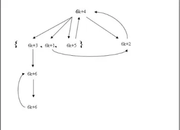
In brief, we present their relations by two graphs:

Figure 3: The number relation in the 3n + 1 backward iteration net.

(20)

2.4 The Total Number Relations Between Consecutive Levels in

The 3n + 1 Backward Iteration Net

In this subsection, by use of the relations between natural numbers under one transformation on I in the 3n + 1 backward iteration net, we classify the total number relations of A to F in two consecutive levels. We list some notations of the 3n + 1 backward iteration net.

Li : The ith level, i = 0, 1, 2, 3, . . .;

Li(N ) : The total natural numbers in Li;

Li(A) : The total numbers of A in Li;

Li(B) : The total numbers of B in Li;

Li(C) : The total numbers of C in Li;

Li(D) : The total numbers of D in Li;

Li(E) : The total numbers of E in Li;

Li(F ) : The total numbers of F in Li.

Then, the total number relations of A to F in two consecutive levels as follows: 1. Li(D) = Li+1(A) + Li+1(C) + Li+1(E).

proof : By the relations of numbers in the backward iteration net, we have:

(1) da→ {b, a}; dc → {b, c}; de→ {b, e}.

(2) Moreover, the previous step of a must be da. The previous step is the original 3n + 1

rules. C(a) = C(6k + 1) = 3(6k + 1) + 1 = 18k + 4 ∈ Da, that is, there exists a

da= 18k + 4 ∈ Da s.t. C(a) = da. Similarly, the previous step of c must be dc, and the

previous step of e must be de.

By (1) and (2) We have:

Li+1(A) = Li(Da); Li+1(C) = Li(Dc); Li+1(E) = Li(De).

Li(D) = Li(Da) + Li(Dc) + Li(De) = Li+1(A) + Li+1(C) + Li+1(E).

2. Li(B) + Li(E) = Li+1(D).

(21)

(2) Moreover, the previous step of d must be b or e. The previous step is the original 3n + 1 rules. Since d = 6k + 4∈ even, for some k ∈ N, C(d) = (6k + 4)/2 = 3k + 2.

Now we consider k:

Case 1: If k = 2m, m∈ N, then C(d) = 3k + 2 = 3 · (2m) + 2 = 6m + 2 ∈ B.

Case 2: If k = 2m + 1, m∈ N ∪ {0}, then C(d) = 3k + 2 = 3 · (2m + 1) + 2 = 6m + 5 ∈ E. By (1) and (2): We have Li(B) + Li(E) = Li+1(D).

3. Li(A) + Li(D) = Li+1(B).

(1) a→ b and d → b.

(2) Moreover, the previous step of b must be a or d. The previous step is the original 3n + 1 rules. Since b = 6k + 2∈ even, for some k ∈ N, C(d) = (6k + 2)/2 = 3k + 1.

Case 1: If k = 2m, m∈ N. Then C(b) = 3k + 1 = 3 · (2m) + 1 = 6m + 1 ∈ A.

Case 2: If k = 2m + 1, m∈ N. Then C(b) = 3k + 1 = 3 · (2m + 1) + 1 = 6m + 4 ∈ D. By (1) and (2): We have Li(A) + Li(D) = Li+1(B).

4. Li(C) + Li(F ) = Li+1(F ).

(1) c→ f and f → f.

(2) Moreover, the previous step of f must be c or f. The previous step is the original 3n + 1 rules. Since f = 6k + 6∈ even, for some k ∈ N, C(f) = (6k + 6)/2 = 3k + 3.

Case 1: If k = 2m, m∈ N, then C(f) = 3k + 3 = 3 · (2m) + 3 = 6m + 3 ∈ C.

(22)

By (1) and (2): We have Li(C) + Li(F ) = Li+1(F ).

5. Li(N ) + Li(D) = Li+1(N ).

proof : By the relations of numbers in 3n + 1 backward iteration net, we have: under one

transformation on I, a, b, c, e, f , will iterate to only one natural number respectively. However, for d ∈ D, d will iterate to two diﬀerent natural numbers under one transformation on I. Hence, the extra numbers of Li+1 more than Li+1 equals Li(D). That is, Li(N ) + Li(D) =

Li+1(N ).

2.5 Properties

In this subsection, we will show the relation between Collatz function C(n) and its inverse operator, I(n). This helps us realize the relations among more natural numbers in the 3n + 1 backward iteration net.

Remark 2.3. For p, q∈ N, if C(p) = q, then p ∈ I(q).

proof : We will prove it by considering p.

Case 1: If p = 6k, for some k ∈ N, since C(p) = C(6k) = (6k)/2 = 3k = q, then I(q) = I(3k) =

{2(3k)} = {6k}. Thus, p ∈ I(q).

Case 2: If p = 6k +1, for some k ∈ N∪{0}, since C(p) = C(6k+1) = 3(6k+1)+1 = 18k+4 = q, then I(q) = I(18k + 4) ={(18k+4)₃ −1, 2(18k + 4)} = {6k + 1, 36k + 8}. Thus, p ∈ I(q).

Case 3: If p = 6k + 2, for some k ∈ N ∪ {0}, since C(p) = C(6k + 2) = (6k + 2)/2 = 3k + 1 = q, then I(q) = I(3k + 1) ={2(3k + 1)} = {6k + 2}. Thus, p ∈ I(q).

Case 4: If p = 6k+3, for some k ∈ N∪{0}, since C(p) = C(6k+3) = 3(6k+3)+1 = 18k+10 = q, then I(q) = I(18k +10) ={(18k+10)₃ −1, 2(18k +10)} = {6k+3, 36k+20}. Thus, p ∈ I(q).

Case 5: If p = 6k + 4, for some k ∈ N ∪ {0}, since C(p) = C(6k + 4) = (6k + 4)/2 = 3k + 2 = q, then I(q) = I(3k + 2) ={2(3k + 2)} = {6k + 4}. Thus, p ∈ I(q).

Case 6: If p = 6k+5, for some k ∈ N∪{0}, since C(p) = C(6k+5) = 3(6k+5)+1 = 18k+16 = q, then I(q) = I(18k +16) ={(18k+16)₃ −1, 2(18k +16)} = {6k+5, 36k+32}. Thus, p ∈ I(q).

(23)

Because Case 1 to Case 6 all hold, we claim the remark.

Remark 2.4. For p, q∈ N, if p ∈ I(q), then C(p) = q.

proof : We will prove it by considering q.

Case 1: If q = 6k, for some k ∈ N, since I(q) = I(6k) = {2(6k)} = {12k} and p ∈ I(q), then

p = 12k. Thus, C(p) = C(12k) = (12k)/2 = 6k = q.

Case 2: If q = 6k + 1, for some k ∈ N ∪ {0}, since I(q) = I(6k + 1) = {2(6k + 1)} = {12k + 2} and p∈ I(q), then p = 12k + 2. Thus, C(p) = C(12k + 2) = (12k + 2)/2 = 6k + 1 = q. Case 3: If q = 6k + 2, for some k ∈ N, since I(q) = I(6k + 2) = {2(6k + 2)} = {12k + 4} and

p∈ I(q), then p = 12k + 4. Thus, C(p) = C(12k + 4) = (12k + 4)/2 = 6k + 2 = q.

Case 4: If q = 6k + 3, for some k ∈ N, since I(q) = I(6k + 3) = {2(6k + 3)} = {12k + 6} and

Case 5: If q = 6k + 4, for some k ∈ N, since I(q) = I(6k + 4) = {(6k+4)₃ −1, 2(6k + 4)} = {2k + 1, 12k + 8} and p ∈ I(q), then p = 2k + 1 or p = 12k + 8. Now we consider the

two conditions:

Subcase 1: If p = 2k + 1, then C(p) = C(2k + 1) = 3(2k + 1) + 1 = 6k + 4 = q. Subcase 2: If p = 12k + 8, then C(p) = C(12k + 8) = (12k + 8)/4 = 6k + 4 = q.

By Subcase 1 and Subcase 2, the Case 5 holds.

Case 6: If q = 6k + 5, for some k ∈ N, since I(q) = I(6k + 5) = {2(6k + 5)} = {12k + 10} and

Because Case 1 to Case 6 all hold, we claim the remark.

Proposition 2.5. If q ∈ N, then I(q) = {p| C(p) = q, p ∈ N}.

proof : By Remark 2.3 and Remark 2.4, we have: for p, q ∈ N, C(p) = q if and only if p∈ I(q). That is, I(q) = {p| C(p) = q}.

(24)

In Proposition 2.5, we know the relation between C(n) and I(n) under one transformation. In the following, by use of Remark 2.3 and Remark 2.4, we will show the relation between

C(n) and I(n) under k transformations.

Remark 2.6. For p, q, k ∈ N, if C(k)_{(p) = q, then p}_{∈ I}(k)_(q).

proof : For p, q, k ∈ N, if C(k)_{(p) = q, then there exists a ﬁnite trajectory P on C(n) with}

starting value p and length k, such that

P = (p, p1, p2, . . . , pk−1, q), pi = C(i)(p), i = 1, 2, 3, . . . , k− 1.

Since C(p) = p1, by Remark 2.3, we have p ∈ I(p1). Similarly, we know p1 ∈ I(p2), p2 ∈

I(p3), . . ., pk−2 ∈ I(pk−1), and pk−1 ∈ I(q). By the relations, we have:

p∈ I(p1)⊆ I(I(p2))⊆ I(I(I(p3))) ⊆ · · · ⊆ I(k−1)(pk−1)⊆ I(k)(q).

Hence, p∈ I(k)(q).

Remark 2.7. For p, q, k ∈ N, if p ∈ I(k)(q), then C(k)(p) = q.

proof : For p, q, k ∈ N, if p ∈ I(k)(q), then there exists a path Q on I in βk(q) with length k,

such that

Q = (q → q1 → q2 → · · · → qk−1 → p), qi ∈ I(i)(q), i = 0, 1, 2, 3, . . . , k− 1.

Moreover, by Remark 2.4, we have q = C(q1), q1 = C(q2), . . ., qk−2 = C(qk−1), and

qk−1 = C(p). Thus,

q = C(q1) = C(C(q2)) =· · · = C(k−1)(qk−1) = C(k−1)(C(p)) = C(k)(p).

Proposition 2.8. If q ∈ N, then I(k)_{(q) =}_{{p| C}(k)_{(p) = q, p}_{∈ N}.}

proof : By Remark 2.6 and Remark 2.7, we have: for p, q ∈ N, C(k)_{(p) = q if and only if}

p∈ I(k)_{(q). That is, I}(k)_{(q) =}{p| C(k)_{(p) = q}}.

In Proposition 2.8, we realize the meaning of Ik(n), that is, by use of Ik(n), we can collect all the natural numbers which iterate to n under exactly k transformations on Collatz function. In section 2, we introduce the 3n + 1 backward iteration net, and the relation of the natural numbers in the net. However, for our initial idea, we wonder if 1 can strength all the natural numbers set. Thus, in section 3, we focus on a particular 3n + 1 backward iteration net.

(25)

3 A Particular 3n + 1 Backward Iteration Net β

_k

(8)

For our initial idea: if we let 1 be the starting value and make use of the 3n + 1 backward iteration formula I, can we strength all the natural numbers set N? Therefore, βk(1) is the

main net what we interested in. However, we ﬁnd that there is a trivial cycle 1→ 2 → 4 → 1 in βk(1). For simplifying our work, the main net what we research transformed into βk(8).

Why do we choose βk(8)? Because observing βk(1), we ﬁnd that our initial idea is equal to

the following idea: if we let 8 be the starting value and make use of the 3n + 1 backward iteration formula I, can we strength N \ {1, 2, 4}? Thus, in this section, βk(8) is the main

3n + 1 backward iteration net what we research. In this section, we will introduce βk(8) and

some properties in βk(8).

3.1 Some Records of β

k

(8)

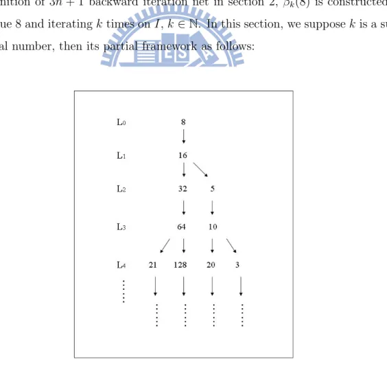
By the deﬁnition of 3n + 1 backward iteration net in section 2, βk(8) is constructed by the

starting value 8 and iterating k times on I, k ∈ N. In this section, we suppose k is a suﬃcient large natural number, then its partial framework as follows:

(26)

For convenience, we let I(i)(8) be Li, called level i, i = 0, 1, 2,. . . , k. In the following, we

list the ﬁrst 12 levels of βk(8):

L0 : 8. L1 : 16. L2 : 5, 32. L3 : 10, 64. L4 : 3, 20, 21, 128. L5 : 6, 40, 42, 256. L6 : 12, 13, 80, 84, 85, 512. L7 : 24, 26, 160, 168, 170, 1024. L8 : 48, 52, 53, 320, 336, 340, 341, 2048. L9 : 96, 17, 104, 106, 640, 672, 113, 680, 682, 4096. L10: 192, 34, 208, 35, 212, 213, 1280, 1344, 226, 1360, 227, 1364, 1365, 8192. L11: 384, 11, 68, 69, 416, 70, 424, 426, 2560, 2688, 75, 452, 453, 2720, 454, 2728, 2730, 16384.

In the following, for our best, we record L0 to L59 in βk(8), by Appendix A. Being

ac-companied the increasing level, the total number Li(N ) will be larger and larger. Therefore,

we want to know the total number growing rate to realize βk(8) more. We analysis the total

number growing rate in βk(8) as follows:

The total number growing rate Li(N )/Li−1(N ):

Owing to the proposition in 2.4: Li+1(N )− Li(N ) = Li(D) and Li(D) ≥ 0. Therefore,

we have Li(N )/Li−1(N ) ≥ 1. From L0 to L10, the growing rate varies much, falls in [1, 2].

However, accompanied the increasing level, the growing rate seems more and more stable. From L25 to L59, the growing rate all falls in (1.25, 1.27). Moreover, From L43 to L59, the

growing rate all falls in (1.263, 1.265).

Although we just record L0 to L59 in βk(8), by the analysis of the total number growing rate,

we have some sense of total number in βk(8). Moreover, according the growing rate trend, if

(27)

3.2 Properties

In this subsection, by use of the remarks and propositions in 2.5, we will classify the properties in βk(8) more precisely.

Remark 3.1. In βk(8), 2n+3∈ Ln, for n = 0, 1, 2, . . . , k.

proof : We will prove it by mathematical induction.

(i) When n = 0, 23 _{= 8}_{∈ L}

0. True!

(ii) Suppose n = m, m < k, 2m+3 ∈ L

m is true. Then by the formula I(n), we have:

∃m1 ∈ Lm+1 s.t. m1 = I(2m+3) = 2· 2m+3 = 2m+4. Therefore, 2m+4 ∈ Lm+1. True!

By mathematical induction, we prove it!

Remark 3.1 presents a trivial fact about 2-power natural numbers in βk(8).

Remark 3.2. In βk(8), the elements in Li are distinct, i≤ k.

proof : If p∈ Li, then by Remark 2.7, we have: C(i)(p) = 8, i≤ k. Suppose there exist two

ﬁnite trajectories X, Y with the same length i on Collatz function such that

X = (p, p1, p2, . . . , pi−1, 8), C(n)(p) = pn, n = 0, 1, 2, . . . , i− 1.

Y = (p, q1, q2, . . . , qi−1, 8), C(n)(p) = qn, n = 0, 1, 2, . . . , i− 1.

Since Collatz function, C(1)_{(p) = p}

1 = q1, C(2)(p) = p2 = q2, similarly, pi = qi, for

i = 1, 2, . . . , i− 1. That is, X ≡ Y . Thus, it shows that every element p in Li exists an

unique ﬁnite trajectory with length i from p to 8 on Collatz function. Therefore, the elements in Li are distinct.

Remark 3.3. In βk(8), if p∈ Ls and p∈ Lt, then s = t.

proof : Suppose s̸= t and p ∈ Ls, p∈ Lt, without loss of generality, we let s < t ≤ k, then

by Remark 2.7, we have: C(s)(p) = 8 and C(t)(p) = 8. Therefore, there exist a trajectory S with length s and a trajectory T with length t on Collatz function such that

(28)

T = (p, q1, q2, . . . , qt−1, 8), C(i)(p) = qi, i = 0, 1, 2, . . . , t− 1.

Since Collatz function, C(1)(p) = p1 = q1, C(2)(p) = p2 = q2, similarly, pi = qi, for

i = 1, 2, . . . , s− 1. Thus, T can be written as

T = (p, p1, p2, . . . , ps−1, 8, qs+1, qs+2, . . . , qt−1, 8).

Now we consider the ﬁnite trajectory (8, qs+1, qs+2, . . . , qt−1, 8) in T . Since C(1)(8) = 4,

C(2)(8) = 2, C(3)(8) = 1, C(4)(8) = 4, and so on. That is, qi ∈ {1, 2, 4} for i > s. Thus, the

ﬁnite trajectory (8, qs+1, qs+2, . . . , qt−1, 8) does not exist. It is contradiction to our

assumption. Hence, we prove it!

Remark 3.4. In βk(8), the elements in V (βk(8)) are distinct.

proof: By Remark 3.3, we know that every element belongs to an unique level. Moreover, by

Remark 3.2, we know the elements in a level are distinct. Therefore, the elements in

V (βk(8)) are distinct.

Theorem 3.5. For k ∈ N, there is no cycle in βk(8).

proof: By Remark 3.4, we know: the elements in V (βk(8)) are distinct. Therefore, there is

no cycle in βk(8).

The Theorem 3.5 reveals a fact: For any n ∈ N \ {1, 2, 4}, if n can iterate to 1 on Collatz function, before getting to 1 at ﬁrst time, then n don’t enter any cycle. It matches the fact we have known.

About our initial idea: if we let 8 be the starting value and make use of the 3n + 1 backward iteration formula, can we strength N \ {1, 2, 4}? Although we still don’t know whether the idea is right or not, we get some results in βk(8). In 3.1, we know that if k → ∞, then the

total number in βk(8) have the chance to meet N \ {1, 2, 4}. In 3.2, we know all the natural

numbers are diﬀerent in βk(8). Moreover, in Theorem 3.5, we know there is no cycle in βk(8).

Through the research of βk(8), we have another way to examine and interpret some facts

(29)

4 Simulation Backward Iteration Net

In this section, in order to know more about βk(8), we construct a simulation expected matrix

E to create a simulation backward net. We take the simulation backward net compared with βk(8) on three parts: total numbers, total number growing rate, and the ratio of A to F in

every level. We will introduce E and how we use E to simulate βk(8). Moreover, we take

another four diﬀerent simulation expected value matrices to simulate βk(8). In the end, we

analysis the simulation results and make conclusions.

4.1 Simulation Expected Value Matrix E

In the subsection, we introduce the simulation expected value matrix E. The idea of E is from the relations of numbers in 3n + 1 backward iteration net. In section 2, we realize the natural number relations are a to b, b to d, c to f , e to d, f to f under one transformation on

I. Based on the relations, we construct the simulation expected value matrix E. Especially, d

may be to{a, b},{c, b}, or {e, b} under one transformation on I. Therefore, in E, we suppose the expected value of d to a, c, or e is 1/3 respectively under one transformation. It is more precise description below:

E =               0 0 0 1/3 0 0 1 0 0 1 0 0 0 0 0 1/3 0 0 0 1 0 0 1 0 0 0 0 1/3 0 0 0 0 1 0 0 1               .

We will explain E by columns: (1) The ﬁrst column:

[

0 1 0 0 0 0 ]T

.

The ﬁrst column is a-column. It shows that the expected value of “a iterating to b under one transformation” is 1. Moreover, the expected value of “a iterating to a, c, d, e, or f under one transformation on I” is 0 respectively.

(2) The second column: [

0 0 0 1 0 0 ]T

.

The second column is b-column. It shows that the expected value of “b iterating to d under one transformation” is 1. Moreover, the expected value of “b iterating to a, b, c, e, or f under one transformation ” is 0 respectively.

(30)

(3) The third column: [

0 0 0 0 0 1 ]T

.

The third column is c-column. It shows that the expected value of “c iterating to f under one transformation” is 1. Moreover, the expected value of “c iterating to a, b, c, d, or e under one transformation” is 0 respectively.

(4) The fourth column: [

1/3 1 1/3 0 1/3 0 ]T

.

The fourth column is d-column. It shows that the expected value of “d iterating to b under one transformation” is 1. Moreover, the expected value of “d iterating to d, or f under one transformation” is 0. Especially, the expected value of “d iterating to a, c, or e under one transformation” is 1/3 respectively. (5) The ﬁfth column: [ 0 0 0 1 0 0 ]T .

The ﬁfth column is e-column. It shows that the expected value of “e iterating to d under one transformation” is 1. Moreover, the expected value of “e iterating to a, b, c, e, or f under one transformation” is 0 respectively.

(6) The sixth column: [

0 0 0 0 0 1 ]T

.

The sixth column is f-column. It shows that the expected value of “f iterating to f under one transformation” is 1. Moreover, the expected value of “f iterating to a, b, c, d, or e, under one transformation” is 0 respectively.

Besides E, we also deﬁne identity vectors Xa, Xb, Xc, Xd, Xe, Xf.

Xa= (1, 0, 0, 0, 0, 0)T; Xb = (0, 1, 0, 0, 0, 0)T; Xc = (0, 0, 1, 0, 0, 0)T; Xd= (0, 0, 0, 1, 0, 0)T; Xe= (0, 0, 0, 0, 1, 0)T; Xf = (0, 0, 0, 0, 0, 1)T.

Xa shows that we choose a as starting value and make the 3n + 1 backward iteration

process. So do Xb, Xc, Xd, Xe, Xf. In the following, we take examples to explain how E and

(31)

Example 4.1. E(1)_{∗ X} d= [ 1/3 1 1/3 0 1/3 0 ]T .

It shows: If we choose d as starting value, under one transformation by E, the expected

values of a is 1/3, of b is 1, of c is 1/3, of d is 0, of e is 1/3, of f is 0. That is, under one

transformation by E, the next ﬁrst level of starting value d consists 1/3· a, 1 · b, 1/3 · c, 0 · d, 1/3· e, and 0 · f. Example 4.2. E(2)∗ X d= [ 0 1/3 0 4/3 0 1/3 ]T .

It shows: If we choose d as starting value, under two transformations by E, the expected

values of a is 0, of b is 1/3, of c is 0, of d is 4/3, of e is 0, of f is 1/3. That is, under two

transformations by E, the next second level of starting value d consists 0· a, 1/3 · b, 0 · c, 4/3· d, 0 · e, 1/3 · f. Example 4.3. E(3)_{∗ X} d= [ 4/9 4/3 4/9 1/3 4/9 1/3 ]T .

It shows: If we choose d as starting value, under three transformations by E, the expected

values of a is 4/9, of b is 4/3, of c is 4/9, of d is 1/3, of e is 4/9, of f is 1/3. That is, under

three transformations by E, the next third level of starting value d consists 4/9· a, 4/3 · b, 4/9· c, 1/3 · d, 4/9 · e, 1/3 · f.

In the following, we will introduce that how we use E to simulate βk(8).

4.2 The Simulation Backward Iteration Net

In this subsection, we will introduce the simulation backward iteration net constructed by

E and Xb, then we use it to compare with βk(8). In our simulation work, we suppose the

expected value of d to a, c, or e is 1/3 respectively under one transformation by E. But in

βk(8), the behavior of d under one transformation on I is deterministic. Therefore, in the

simulation backward iteration net by E, we take the expected value of A to F in every level as our simulation object. Since our simulation aim is βk(8) and 8 ∈ B, we choose b as

our simulation starting value. Thus, we use E and Xb to construct the simulation backward

iteration net. The net compared with βk(8) is focused on three parts: total numbers, total

number growing rate, and the ratios of Li(A), Li(B), Li(C), Li(D), Li(E), and Li(F ) to

Li(N ) respectively in every level. We try our best to simulate βk(8) with 60 levels (L0− L59).

In the following, we will introduce the simulation process and results.

(32)

Step 1: Owing to the simulation aim is βk(8), the starting value 8 belongs to B. Therefore, we

choose E and Xb to construct the simulation backward iteration net.

Step 2: For βk(8), let L0 be the starting value 8, L1 be {16}, L2 be {5, 32}, and so on. For our

simulation backward iteration net, let L0 be b, L1 be E(1)∗ Xb, L2 be E(2)∗ Xb, and so

on.

Step 3: For our best, we can record the total numbers of L0 to L59 in βk(8). On the other hand,

for our simulation backward iteration net, we take the sum of E(i) _{∗ X}

b as the total

expected value in Li, denoted Ei(N ), i = 0, 1, 2, . . . , 59.

Step 4: We compare them for (Ei(N )− Li(N )), i = 0, 1, 2, . . . , 59.

For convenience, we denote Di(N ) = Ei(N )−Li(N ). By Appendix B, the results as follows:

Di(N ): From L0 to L3, Di(N ) all are 0. But from L4, Di(N ) is not equal to 0 anymore. From

L4 to L15, Di(N ) may be positive or negative, and the absolute value of Di(N ) less

than 2. From L16 to L59, surprisingly, we found that Di(N ) is positive and increasing.

D16(N ) is about 0.5 , but D59(N ) is about 65022.4.

In a word, accompanied by the increasing level, we can conclude that the Di(N ) will

be larger and larger. That is to say, on the total numbers, the simulation backward iteration net constructed by E and Xb will be further and further than βk(8).

The Second way: Total number growing rate in every level.

The simulation process is similar to total numbers simulation. For convenience, we denote

Li(N )/Li−1(N ) as the total number growing rate of βk(8), denote Ei(N )/Ei−1(N ) as the total

expected value growing rate of the simulation backward iteration net, and denote Ki(N ) =

|(Ei(N )/Ei−1(N ))−(Li(N )/Li−1(N ))| as the absolute value of the diﬀerence between the two

growing rates. By Appendix B, the results as follows:

Ki(N ): L0− L9: the minimum Ki(N ) is 0, the maximum Ki(N ) is 0.33333.

L10− L19: the minimum Ki(N ) is 0.01093, the maximum Ki(N ) is 0.0605.

(33)

In a word, accompanied by the increasing level, on average, the Ki(N ) trends smaller

and smaller. That is, on the total number growing rate in every level, the simulation backward iteration net by E and Xb will be closer and closer than βk(8).

The third way: The ratios of Li(A), Li(B), Li(C), Li(D), Li(E), and Li(F ) to Li(N )

respectively in every level.

Step 1: Owing to the simulation aim is βk(8), 8 is the starting value and belongs to B. Therefore,

we choose E and Xb to construct the simulation backward iteration net.

Step 2: For βk(8), let L0 be the starting value 8, L1 be {16}, L3 be {5, 32}, and so on. For our

simulation backward iteration net, let L0 be b, L1 be E(1)∗ Xb, L2 be E(2)∗ Xb, and so

on.

Step 3: For our best, we can record the ratio of A, B, C, D, E, F from L0 to L59 respectively

in βk(8). We denote Ri(A) represents the ratio of Li(A) to Li(N ), and so do Ri(B),

Ri(C), Ri(D), Ri(E),and Ri(F ). For the convenience on comparison, we let:

Ri(A) = (Li(A)/Li(N ))× 100; Ri(B) = (Li(B)/Li(N ))× 100; Ri(C) = (Li(C)/Li(N ))× 100; Ri(D) = (Li(D)/Li(N ))× 100; Ri(E) = (Li(E)/Li(N ))× 100; Ri(F ) = (Li(F )/Li(N ))× 100.

On the other hand, in the simulation backward iteration net, in Li, the ﬁrst entry of

E(i)∗ X

b represents the expected value of A, denoted Ei(A). Similarly, the second entry

represents the expected value of B in Li, denoted Ei(B), and so do Ei(C), Ei(D), Ei(E),

and Ei(F ). Moreover, we denote Wi(A) represents the ratio of Ei(A) to Ei(N ), and so

do Wi(B), Wi(C), Wi(D), Wi(E),and Wi(F ). For the convenience on comparison, we

let: Wi(A) = (Ei(A)/Ei(N ))× 100; Wi(B) = (Ei(B)/Ei(N ))× 100; Wi(C) = (Ei(C)/Ei(N ))× 100; Wi(D) = (Ei(D)/Ei(N ))× 100; Wi(E) = (Ei(E)/Ei(N ))× 100; Wi(F ) = (Ei(F )/Ei(N ))× 100.

(34)

Step 4: For the ratio comparisons, we take absolute value of every ratio error, and we observe the maximum ratio error in every level. The notations as follows:

Yi(A) = |Wi(A)− Ri(A)|;

Yi(B) =|Wi(B)− Ri(B)|;

Yi(C) =|Wi(C)− Ri(C)|;

Yi(D) =|Wi(D)− Ri(D)|;

Yi(E) =|Wi(E)− Ri(E)|;

Yi(F ) =|Wi(F )− Ri(F )|;

Yi(M ) = max{Yi(A), Yi(B), Yi(C), Yi(D), Yi(E), Yi(F )}.

Step 5: We compare them by use of Yi(M ), i = 0, 1, 2, . . . , 59.

By Appendix C and Appendix D, the results as follows:

L0− L9: the maximum Yi(M ) is 36.66667. L10− L19: the maximum Yi(M ) is 10.53939. L20− L29: the maximum Yi(M ) is 2.20515. L30− L39: the maximum Yi(M ) is 0.70776. L40− L49: the maximum Yi(M ) is 0.28697. L50− L59: the maximum Yi(M ) is 0.05015.

In a word, accompanied by the increasing level, on average, the Yi(M ) trends smaller and

smaller. That is to say, on the ratios of Li(A), Li(B), Li(C), Li(D), Li(E), and Li(F ) to

Li(N ) respectively in every level, the simulation backward iteration net by E and Xb will be

closer and closer than βk(8).

In this subsection, we use E and Xb to construct the simulation backward iteration net and

compared with βk(8). Accompanied by the increasing level, the total number simulation is

further and further, however, on average, total number growing rate and the ratio simulation are closer and closer. It reveals that the framework of A to F in every level seems similar. Although we take the expected value to simulate, the assumption of d to a, c, e is 1/3 respectively under one transformation by E which may be meaningful.

4.3 Other Simulation Backward Iteration Nets

In this subsection, we take another four diﬀerent expected value matrices and use them to construct four diﬀerent simulation backward iteration nets to simulate βk(8). In E, we

(35)

Because we have the fact that the sum of expected value of d to a, c, and e is 1 under one transformation on I. Therefore, we modify the expected value of d to a, c, and e rather than 1/3, 1/3, 1/3. The modify expected value matrix P is below:

P =               0 0 0 x 0 0 1 0 0 1 0 0 0 0 0 y 0 0 0 1 0 0 1 0 0 0 0 z 0 0 0 0 1 0 0 1               .

x: The expected value of d to a under one transformation, 0 < x < 1. y: The expected value of d to c under one transformation, 0 < y < 1.

z: The expected value of d to e under one transformation, 0 < z = 1− x − y < 1.

Key: x + y + z = 1 means that the sum of expected value of d to a, c, and e is 1 under one

transformation on I.

In the simulation backward iteration net constructed by E and Xb, we ﬁnd the total

ex-pected value growing rate will nearly equal the maximum absolute value of eigenvalues of

E (about 1.2637626) if the level i is suﬃcient large (about larger than 100). On the other

hand, we observe the total number growing rate of L50 to L59 in βk(8). Therefore, we write a

program to get some sets of (x, y, z) of P whose maximum eigenvalues falls in (1.2632, 1.2638). The four diﬀerent simulation expected value matrices which we choose as follows:

(1) P1: (x, y, z) = (1₃ + 0.0001,1₃ − 0.0001,1₃).

(2) P2: (x, y, z) = (1₃ − 0.0001,1₃ + 0.0001,1₃).

(3) P3: (x, y, z) = (1₃ + 0.0002,1₃ − 0.0002,1₃).

(4) P4: (x, y, z) = (1₃ − 0.0002,1₃ + 0.0002,1₃).

The simulation process by P is similar to E, we will compare them by three ways: total numbers, total number growing rate, and the ratios of Li(A), Li(B), Li(C), Li(D), Li(E),

and Li(F ) to Li(N ) respectively in every level. In the following, we will introduce the four

(36)

4.3.1 The simulation results of P1

Case 1. P1: (x, y, z) = (1₃ + 0.0001,1₃ − 0.0001,1₃). The results as follows: (A)Total numbers in every level:

For consistence, we use the same notations which are used on the E simulation. Di(N ) =

Pi(N )− Li(N ). By Appendix E, the results as follows:

Di(N ): From L0 to L3, Di(N ) all are 0. But from L4, Di(N ) is not equal to 0 anymore. From L4

to L15, Di(N ) may be positive or negative, and the absolute value of Di(N ) less than 2.

However, from L16 to L59, surprisingly, we found that Di(N ) is positive and increasing.

D16(N ) is about 0.5, but D59(N ) is about 66679.3.

be larger and larger. That is to say, on the total numbers, the simulation backward iteration net constructed by P1 and Xb will be further and further than βk(8).

(B)Total number growing rate in every level:

For consistence, we use the same notations which are used on the E simulation. Ki(N ) =

|(Ei(N )/Ei−1(N ))− (Li(N )/Li−1(N ))|. By Appendix E, the results as follows:

and smaller. That is, on the total number growing rate in every level, the simulation backward iteration net constructed by P1 and Xb will be closer and closer than βk(8).

(C)The ratios of Li(A), Li(B), Li(C), Li(D), Li(E), and Li(F ) to Li(N ) respectively

in every level:

For consistence, we use the same notations which are used on the E simulation. By Appendix

C and Appendix F, the results as follows:

L0− L9: the maximum Yi(M ) is 36.67067.

(37)

Li(N ) respectively in every level, the simulation backward iteration net constructed by P1

and Xb will be closer and closer than βk(8).

4.3.2 The simulation results of P2

Case 2. P2: (x, y, z) = (1₃ − 0.0001,1₃ + 0.0001,1₃). The results as follows: (A)Total numbers in every level:

Pi(N )− Li(N ). By Appendix G, the results as follows:

than 2. However, from L16 to L59, surprisingly, we found that Di(N ) is positive and

increasing. D16(N ) is about 0.4 , but D59(N ) is about 63367.4.

In a word, accompanied by the increasing level, the Di(N ) will be larger and larger.

That is to say, on the total numbers, the simulation backward iteration net constructed by P2 and Xb will be further and further than βk(8).

|(Ei(N )/Ei−1(N ))− (Li(N )/Li−1(N ))|. By Appendix G, the results as follows:

and smaller. That is, on the total number growing rate in every level, the simulation backward iteration net constructed by P2 and Xb will be closer and closer than βk(8).

(38)

(C)The ratios of Li(A), Li(B), Li(C), Li(D), Li(E), and Li(F ) to Li(N ) respectively

in every level:

For consistence, we use the same notations which are used on the E simulation. By Appendix

C and Appendix H, the results as follows:

L0− L9: the maximum Yi(M ) is 36.66267. L10− L19: the maximum Yi(M ) is 10.53865. L20− L29: the maximum Yi(M ) is 2.2068. L30− L39: the maximum Yi(M ) is 0.70926. L40− L49: the maximum Yi(M ) is 0.28637. L50− L59: the maximum Yi(M ) is 0.04866.

Li(N ) respectively in every level, the simulation backward iteration net constructed by P2

and Xb will be closer and closer than βk(8).

4.3.3 The simulation results of P3

Case 3. P3: (x, y, z) = (1₃ + 0.0002,1₃ − 0.0002,1₃). The results as follows: (A)Total numbers in every level:

Pi(N )− Li(N ). By Appendix I, the results as follows:

than 2. However, from L16 to L59, surprisingly, we found that Di(N ) is positive and

increasing. D16(N ) is about 0.5 , but D59(N ) is about 68338.1.

be larger and larger. That is to say, on the total numbers, the simulation backward iteration net constructed by P3 and Xb will be further and further than βk(8).

|(Ei(N )/Ei−1(N ))− (Li(N )/Li−1(N ))|. By Appendix I, the results as follows:

應用逆推網絡在克拉茲猜想的探討

國

立

交

通

大

學

應

用

數

學

系

碩

士

論

文

應用逆推網絡在克拉茲猜想的探討

Study 3n+1 problem in a backward iteration net

研 究 生 : 段

俊

旭

指導教授 : 張

書

銘 博士

應用逆推網絡在克拉茲猜想的探討

Study 3n+1 problem in a backward iteration net

應用逆推網絡在克拉茲猜想的探討

學生 : 段俊旭 指導教授 : 張書銘 博士

國立交通大學應用數學系 (研究所) 碩士班

摘 要

Study 3n + 1 Problem in a Backward Iteration Net

Student: Chun-Hsu Tuan

Advisor: Dr. Shu-Ming Chang

誌 謝

Contents

List of Figures

1

Introduction

1.1

History of 3n + 1 Problem

1.2

Some Definitions and Results for The 3n + 1 Problem

2

The 3n + 1 Backward Iteration Net β

(n)

2.1

Formula

2.2

The 3n + 1 Backward Iteration net β

(n)

2.3

The Relations Between Natural Numbers Under One

Trans-formation On I

2.4

The Total Number Relations Between Consecutive Levels in

The 3n + 1 Backward Iteration Net

2.5

Properties

3

A Particular 3n + 1 Backward Iteration Net β

(8)

3.1

Some Records of β

(8)

3.2

Properties

4

Simulation Backward Iteration Net

4.1

Simulation Expected Value Matrix E

4.2

The Simulation Backward Iteration Net

4.3

Other Simulation Backward Iteration Nets

研究生 : 段

銘博士

學生 : 段俊旭指導教授 : 張書銘博士

摘要

誌謝