Space-decomposition multiplier method for constrained minimization problems

(1)

PERGAMON

An InlOlllOtlonml Joumll

computers &

mathematics

with q~llcatlons

Computers and Mathematics with Applications 41 (2001) 51-62

www.elsevier.nl/locate/camwa

S p a c e - D e c o m p o s i t i o n Multiplier M e t h o d

for Constrained Minimization P r o b l e m s

CHIN-SUNG LIU

Industrial Technology Research Institute

Mechanical Industry Research Laboratories, Hsinchu, Taiwan, R.O.C. CHING-HUAN TSENG

Applied Optimum Design Laboratory, Department of Mechanical Engineering National Chiao Tung University, Hsinchu 30050, Taiwan, R.O.C.

chtseng@cc, nctu. edu. tw

(Received November 1998; revised and accepted April PO00)

A b s t r a c t - - l n this paper, a new multiplier method that decomposes variable space into decomposed spaces is introduced. This method allows constrained minimization problems to be decomposed into subproblems. A potential constraint strategy that uses only part of the constraint set in the decomposed-space subproblems is also presented to increase the efficiency of this n e w space- decomposition multiplier method. Three examples are given to demonstrate this method and the potential constraint strategy. (~) 2001 Elsevier Science Ltd. All rights reserved.

Keywords--Constrained minimization, Decomposition method, Multiplier method.

1.

I N T R O D U C T I O N

In this paper, a space-decomposition multiplier (SDMP) method is proposed for solving the constrained minimization problem

min f(x), (1)

xE~"

subject to

gj(x) ~ O, j = l , . . . , m , (2)

h ~ ( x ) = 0 , S = l , . . . , m ' , (3) where f : Nn __. N, gj : Nn ~ ~, and hs, : Nn ~ N are lower-bounded, continuous functions. The (augmented Lagrangian) multiplier methods introduced by Hestenes [1] and Powell [2] were pop- ular for such constrained minimization problems in the 1980s. Powell showed that the multiplier method can be superior to the penalty function method [2]. The multiplier methods have continuously found their applications in neural networks for constrained problems [3], in neural networks learning rules [4,5], and in mixed-integer, discrete, and continuous optimization [6]. Recently, new

T h e research reported in this paper was supported under a project sponsored by the National Science Council Grant, Taiwan, R.O.C., N S C 85-2732-E-009-010.

(2)

52 C.-S. Liu AND C.-H. TSENG

penalty and multiplier methods have continuously been developed [7]. Although the multiplier method can significantly improve the efficiency of classical penalty function method, it has been shown that other higher-order algorithms, such as the sequential quadratic programming (SQP) method [8], are more efficient than the classical multiplier method [9,10]. However, despite being less efficient, the multiplier method is still superior in some ways that are listed below.

1. Constrained minimization problems can be transformed into unconstrained minimization problems using the multiplier method. Therefore, the unconstrained minimization tech- nique, including decomposition and parallel processing techniques, can be used directly to solve constrained minimization problems.

2. In general, the multiplier method requires less computer storage space, especially when used for large-scale minimization problems.

3. Exact boundary values for g ( x ) and h ( x ) can be found using the multiplier method. Combining all of these advantages and overcoming the inefficiency of the multiplier methods, the space-decomposition multiplier (SDMP) method is proposed in this paper. The SDMP method extends the classical multiplier method using the space-decomposition minimization (SDM) algorithm proposed by Liu and Tseng [11]. The SDM algorithm decomposes the original variable space S E Nn into subspaces, and allows the minimization problem (1) to be decomposed into subproblems that can be solved either singly on a single processor [11] or simultaneously on parallel processors [12]. The SDM algorithm is based on decomposition methods that provide a systematic approach to decompose minimization problems into small-scaled and coupled subproblems. Mul- tilevel optimization methods, whose applications can be found in structure optimizations [13,14] and in mixed-discrete optimization problems [15], are typical hierarchic decomposition methods. It has been shown that multilevel optimization methods can decompose problems into a set of hierarchically related subproblems, while preserving the coupling among the decomposed subproblems [16]. The applications of multilevel optimization methods can be also found in neural networks learning rules [17]. Other decompositionmethods that decompose minimization problems into subproblems directly have also been proposed by Kibardin [18], Mouallif, Nguyen and Strodiot [19]. Recently, Bouaricha and Mord [20] introduced partial separability for large-scale minimization problems. In these studies, the computing efficiency was shown to increase when the original minimization problems could be decomposed into subproblems.

The SDM algorithm is also based on parallel variable distribution techniques. The parallel variable distribution. (PVD) algorithm, proposed by Ferris and Mangasarian [21], and further extended to inexact PVD algorithms by Solodov [22], was a method that distributes q blocks X l , . • •, Xq of variable x among q processors. These q variable blocks are communicated among processors either synchronously or asynchronously. The PVD algorithm provides a mechanism for updating coupled variables among decomposed subproblems. More recently, Fukushima [23] proposed a more general framework that was called the parallel variable transformation (PVT) algorithm. In this algorithm, the variables are transformed into spaces of smaller dimension, which altogether span the space of the original variables. Fukushima [23] showed that the PVD algorithms can be a special case of the general PVT framework.

The notation and terminology used in this paper are described as follows: S E Nn denotes n-dimensional Euclidean design space with ordinary inner product and associated two-norm [[. I[, italic characters denoting variables and vectors. For a differentiable function f : N'~ --~ ~, V f denotes the n-dimensional vector of partial derivatives with respect to x and V f s ~ ( x s , ) denotes the ni-dimensional vector of partial derivatives with respective to xs~ E ~ ' ~ . For simplicity of notation, changes in the ordering of variables are allowed throughout this paper. Therefore, the variable vector x E S can be decomposed into subvectors. That is, x = [ x s l , . . . , x s , , ] , where xs~, i = 1 , . . . , q, are subvector or subcomponent of x.

This paper is organized as follows. In Section 2, basic definitions of the decomposed-space set, decomposed-space minimization function, and decomposed-space constraint set are given.

(3)

Space-Decomposition Multiplier Method 53 In Section 3, the SDM algorithm for unconstrained minimization problems is introduced. In Section 4, convergence criteria are derived. The classical multiplier method and the space- decomposition multiplier method are introduced in Sections 5 and 6, respectively. In Section 7, the potential constraint strategy that uses only a subset of the constraints is proven. Numerical results are presented in Section 8.

2. D E C O M P O S E D - S P A C E S E T

The space-decomposition minimization (SDM) algorithm [11] is a sequential algorithm that can solve minimization problems (1). The decomposed-space set and decomposed-space minimization function defined in [11] are modified as follows for this paper.

DEFINITION 2.1. NONOVERLAPPING DECOMPOSED-SPACE SET. The original variable space S

is spanned by {x [ x E ~n}. If the variable x is decomposed into x = [xs~,..., xs,], then the decomposed space Si, spanned by the subvector {xs~ [ xs~ E Nn~, where ~q=i ni = n}, forms a no.noverlapping decomposed-space s e t { S I , . . . , S q } . That is, Uq=~ Si = S and SiNSj = ~, if i ~t j.

From Definition 2.1, the minimization function (1) can be decomposed as

S(x) = ss, + (4)

where xg~ is the complement vector of xs~, fs~ (xs~, xg~) is the decomposed-space minimization function in the decomposed space Si and f9~ (xg~) is the complement decomposed-space function. COROLLARY 2.2. From (4), f$~ (x9~) is only a function of xg~. Therefore, it can be removed from

the minimization subproblem ff x ~ is invaxiant in the decomposed space Si.

DEFINITION 2.3. DECOMPOSED-SPACE CONSTRAINT SET. The decomposed-space constraint sets gj,s, (xs~, xg~) and hj,,s, (xs~, xg~ ) axe defined as

= gj, , + gj, , <_ o, h i . ( = ) = t,j.,s, + hj. , = o,

j = l , . . . , m , i = l , . . . , q , (5)

j ' = l , . . . , m ' , i = l , . . . , q . (6)

COROLLARY 2.4. From Definition 2.3, the complement decomposed-space constraints gj,~ ( x $~ ) and hj,,~ (xg~) axe only functions of x ~ ; that is, if x ~ is a constant vector, gj,9~ (x$~) and hi,,9 ~ (x$~) will be constant values. Therefore, they need be calculated only once during the minimization process in decomposed space Si.

Step 1. Step 2. Step 3.

3. S P A C E - D E C O M P O S I T I O N

M I N I M I Z A T I O N ( S D M ) A L G O R I T H M

The SDM algorithm is a sequential algorithm that can efficiently solve unconstrained minimization problems on a single processor [11]. In this section, the SDM algorithm is presented in brief without proof. In the following sections, it will be further expanded to the constrained minimization problem (1)-(3).

ALGORITHM 3.1. SPACF~DECOMPOSITION MINIMIZATION (SDM) ALGORITHM.

Decompose the variable space into a nonoverlapping decomposed-space set { $ 1 , . . . , Sq}

and derive the decomposed-space minimization functions fs~ (xs~, x ~ ) , for i = 1 , . . . , q. Choose the starting point x (1), where x0) --Lrx(1)sl ," " , x(1)]sqJ and set k -- 1.

For i = 1 to q, solve one or more steps of the minimization subproblems fs,(x(k),x~)

using any convergent descent algorithm that satisfies

( [x(k) x-'~ )

[X (k) X- ~TA(k) > (71 VfSi [ S, ' S,) > 0 (7)

(4)

54 C.-S. LIU A N D C.-H. T S E N G

and

where al(.), a2(.) are forcing functions [21,23], and d (k) is the search direction in the _s, decomposed space Si.

Step 4. Apply convergence criterion, such as I IV S s, (x(sk,), x~,)II <-- e, to all decomposed spaces Si. If the convergence criterion has been satisfied for all decomposed spaces, the minimum solution has been found as x* =Ix* ... x* 1. sl, , s q , °therwise, set k = k + l and g° to S t e p 3. 4. C O N S T R A I N T V I O L A T I O N A N D C O N V E R G E N C E C R I T E R I A

As shown in [24], two convergence criteria are required for the inner loop and the outer loop of multiplier methods. In the inner loop, the unconstrained minimization convergence criterion is called Lagrangian condition. In the outer loop, the constraint condition is required. For the algorithm presented in this paper, the Lagrangian condition is satisfied first, and then the constraint condition is satisfied.

If the gradient method is used for the decomposed-space subproblem in the inner loop, the Lagrangian condition can be

IIVAII=~~I,VAs,

II2<el.~=I

(9)

In the outer loop, the constraint violation is monitored using the violation criteria for all constraints. Therefore, a maximum constraint violation V (k) is defined as [25]

Y (k) = max{O;gl,... ,gin; I h l l , . . . , Ihm, I} • (10) Therefore, the constraint condition for the outer loop is satisfied when

V (k) _< e2. (11)

If only inequality constraints are presented in the constraint set, the cumulative constraint measure that permits representation of large numbers of inequality constraints by a single cumulative measure can be used. This approach is generally applied to structure optimization and is defined as [261

V (k) = In exp (pgj) , where p is an arbitrarily large number taken between 25 and 50.

(12)

5. A U G M E N T E D L A G R A N G E M U L T I P L I E R M E T H O D

Multiplier methods that combine the penalty function and the Lagrange multiplier A are briefly reviewed before describing the space-decomposition multiplier (SDMP) method. The decomposed-space augmented Lagrangian function is also illustrated in this section.

To solve the constrained minimization problems (1)-(3), the augmented Lagrangia~ function is defined as [27] 7Tt m = :(-)÷

E

÷ [,,(-)+,,'.]' j-=l j=l m ~ m '

+ E [~)+j,hj,(x)] +r(k) E [hy(x)] 2 ,

j ' = l 3'=1 (13)

(5)

Space-Decomposition Multiplier Method 55

A~ k) are the Lagrange multipliers and r (k) is the penalty parameter in the k th iteration. To where

avoid the necessity of having m additional slack variables s5, the augmented Lagrangian function is shown to be equivalent to [28]

A(x) : f ( x ) + Z [A~ k)~j(x)] +r(k)~-~ [aJ (x)]2 + ~ [A(mk)+5'hs'(x)] ÷r(k) Z [h5 '(x)]2' (14)

j = l j = l j ' = l j'----1

where

(

~ ( ~ / =

max g s ( ~ ) , - 2 - - ~ | "

(15)

Therefore, the minimization solution can be found by minimizing the augmented Lagrangian function A(x), with the Lagrange multipliers updated using

)~(k+l) = ~k) +

j 2r(k)(~j(x), j = 1, " ' ' , m, and

(1~)

where a 5 (xs,,x~,) = max gs,s, (xs,,x~,) + gs,gi (x$,) '-2r(k----" ~

(20)

and

hs, (xs,,x~,) = hs,,s, (x~,,~.,) + hs,,~, (~.,) •

(21)

In addition, equations (16),(17) can be modified to

A!k+l) = A~k) + 2r(k)~ 5 (XS, x$~) j = 1 , . . , m , (22)

J ' , *

A(k+l) _{m+5' = "'m+5' +}~(k) 2r(k) _{[hs,,s , (xs,,xg,) + hs,,9 ,}_{(xg,)] ,} j ' _{= 1 , . . . ,}m'. ₍₂₃₎ Therefore, the augmented Lagrangian function (14) can be rewritten as

A(x) = As, (xs,,xa,) + f$, (x~,). (24)

Since fa~(x8~) is a constant value in decomposed space Si, it can be omitted during the minimization process. In addition, gs,~, (xa~) and hs,,a ~ (x~) are also constant values in (20)-(23). Therefore, they need be calculated only once during the minimization process in the decomposed space Si.

A(k+l) _{m T j '} _{= " ' m + j ' -{-}~(k) 2r(k)hj,(x), j ' ₌ 1,... _{' m r "} (17) Then, the penalty parameter r (k) is updated using

r (k+l) = cr (k), (18)

where c > 1 is a constant value. The iterative process in (14)-(18) continues until convergence has been achieved.

From Definitions 2.1 and 2.3, the decomposed-space augmented Lagrangian function that will be used in the following sections can be defined as

m m

j----I j = l

, ,

(19)

(6)

56 C.-S. LIU AND C.-H. TSENG

6.

S P A C E - D E C O M P O S I T I O N M U L T I P L I E R (SDMP) M E T H O D

As shown in the previous sections, the space-decomposition minimization (SDM) algorithm can be applied to the multiplier method and is summarized as the space-decomposition multiplier (SDMP) method. The SDMP method for the constrained minimization problems (1)-(3) includes an outer loop and an inner loop. The outer loop provides a framework for the classical multiplier method, while the inner loop minimizes the augmented Lagrange function (19) using the SDM algorithm. This is summarized as follows.

ALGORITHM 6.1. SPACE-DECOMPOSITION MULTIPLIER ( S D M P ) METHOD. OUTER LOOP.

Step 1. Decompose the variable space S E ~n into q nonoverlapping decomposed spaces

( $ 1 , . . . ,Sq}. Then, derive the q decomposed-space minimization function fs,,

the q decomposed-space constraint sets ga,s~ (xs~, x ~ ) , ha,,s ~ (x8~, xg~), and the q complement decomposed-space constraint sets gj,~ (x~), h a,,3~ (x~), where i = 1 , . . . , q , j = 1 , . . . , m , and j~ = 1 , . . . , m ' .

Step 2. Choose the starting point x (1) , where x(1) = Lrx(1)s~, • • • , x(1)ls,, J and set k = 1. Step 3. Initialize the Lagrange multiplier ~1), the penalty parameter r (1) and the constant

value c > 1. In general, set )~1) = 0, where j = 1 , . . . , (m + m').

INNER LOOP.

Step 4. For i = 1 to q, solve the minimization solution of the augmented La- grange function (19) using any zero or one-order convergent descent algorithm. Then, update x(k '~), which is a subvector of x(k); that is,

X ( k ) __-- [X(kl '1) X ( k ' q ) ]

' " " " ' S ~ J"

Step 5. If the Lagrangian condition (9) has been satisfied, go to Step 6 of the Outer loop; otherwise, go to Step 4 of the inner loop.

Step 6. Update the penalty parameter r (k) by (18) and the Lagrange multiplier )~k) by (22),(23).

Step 7. If the constraint condition (11) has been satisfied, the minimization solution is found asx* = [ s~, ", s~], otherwise, set k = k + 1 and go to Step 4 of the inner x* .. x* • loop.

7.

P O T E N T I A L C O N S T R A I N T

S T R A T E G Y

Numerical algorithms that use only subsets of the constraints are said to use a potential constraint strategy [25]. The main effect of using such a strategy is on the efficiency of the iterative process. This is especially true for large and complex minimization problems that may have hundreds of constraints, but only a few constraints may be in the potential set. In this section, it will be shown that any constraint not in the potential set can be temporarily removed from the constraint set during the iterative process. This elimination of constraints can reduce the dimensions of decomposed-space subproblems and increase the efficiency of the entire algorithm. Therefore, the potential constraint strategy is highly beneficial and should he used in practical optimization applications [25].

To apply the potential constraint strategy to the SDMP method, the constraint set (2),(3) is divided into potential constraint set ~s~ and nonpotential constraint set ~ in decomposed space Si as follows:

= {gJ Ida

v j c { 1 , . . , m } }

and

{hi, I ha'

Vj' c

(25)

and

(7)

Space-Decomposition Multiplier Method 57

That is, the potential constraint set ~s, is constructed by the constraints that are functions of xs, and/or x~,. By contrast, the nonpotential constraint set (s, is constructed by the constraints that are functions of xg~. The potential constraint strategy can be applied to the decomposed-space augmented Lagrangian function (19), and is formulized in the following theorem.

THEOREM 7.1. For the constrained minimization problems (1)-(3), /f any constraint is not in the potential constraint set (s~, it can be temporarily removed from the constraint set in the decomposed space S~.

PROOF. From (5), if g3(x) is a function of only x ~ in decomposed space Si, then

g3(x) = gj,~ (x$~) = constant value in Si.

(27)

Therefore, (15) gives

a3 (x) = constant value in Si. (28)

Similarly, if h i, (x) is a function of only xg~ in the decomposed space Si, from (6), we can also have

hj,(x) = hj,,~ ( x ~ ) = constant value in Si. (29) Therefore, the decomposed-space augmented Lagrangian function (19) can be rewritten as

+r(~)

]~

[hJ'(~,,~e,)] ~+ Z [hj,( ~,)7

hi, E¢s i hi,

ECs~

gj E ¢8 i gj E¢S i

[~(k)

[Am+j"~J' (Xsi , X s i ) ]'4-r(k) +

hi, E~s i hi, E(s i

_ L"m+Y '°3 hi, E¢s~

[~3(xe,)] ~ }

g~ e ¢s~

,~,)]~

(30)

(31)

where

[~?).j (x~,)] + r(~) ~ [.j (x~,)]:

L"mTj, '°3' h~, ~¢s~

[h3, (x~,)] ~

Since x ~ is a constant vector in the decomposed space Si, ¢ ( x ~ ) is also a constant value. Therefore, ¢(xg~) can be removed from (31) without affecting the minimization solutions of the decomposed-space subproblems. That is, the nonpotential constraint set (s~ can be temporarily eliminated from the constraint set in the decomposed space Si. Since only a subset of the constraint set is required to evaluate the minimization solution, the efficiency of the SDMP method can be improved especially for large-scale constraint sets. |

(8)

58 C.-S. LIu AND C.-H. TSENG

From Theorem 7.1, the decomposed-space augmented Lagrangian function (19) can be rewritten as

E

g:i E ~sl g~ E ~s~

(32)

+ E

E

h~, E(s~

h~, E~s~

that can be applied to Step 4 of Algorithm 6.1.

8. I M P L I C I T C O N S T R A I N E D M I N I M I Z A T I O N P R O B L E M

In many mechanical and structural engineering applications, the minimization problem is the weight, mass, or material volume of the designed system. This is usually an explicit function of variables x. Implicit minimization problem, such as stress, displacement, vibration frequencies, etc., can also be treated by introducing artificial variables [25]. Therefore, a general minimization problem can be formulated as an explicit minimization function

f(x)

satisfying the implicit constraints

gj(x,U) <_ O,

j = 1 , . . . , m ,

(33)

h~(~,U) = 0,

j' = 1,...,m',

or the explicit constraints

g~(x) < o, j = 1 , . . . , m ,

(34) h~(x) = 0 , j' = 1,...,m',

where U is an implicit function of x. In some engineering applications, such as the structural systems, the implicit variables U can be expressed as theequilibrium equation

K(x)U = F(x),

(35)

where

K(x)

is a ~ x l stiffness matrix and

F(x)

is an effective load vector having £ components.

The stiffness matrix and effective load vector generally depend explicitly on the variables x. If the one-order descent method is used to minimize the constrained minimization problem, it is necessary to evaluate the gradients of constraint functions. When the constraint functions are implicit in variables x, the special procedures for gradient evaluation are required [25]. From (33) and the chain rule of differentiation, the total derivative of gj with respect to the variables in the decomposed-space Si is given as

~g~

ogj

og7 du

(36)

dzs, = Oxs, + O--ff dzs--,'

where

Og~ _ r og~ Ogj Og~

1 T

ou L OU, ' ou2' " " ou~ j

and

dU = [ dU1 dU2

dUt ]-r

dxs,

[~ss,' d x s , ' " " d x s ,

_J

The partial derivatives ~

_Oxs~

and ~ are easy to calculate. The ~ can be obtained by differ° entiating (35). That is,

(9)

S p a c e - D e c o m p o s i t i o n M u l t i p l i e r M e t h o d 59

Therefore, the dU can be calculated by (37), because the explicit form of K ( x ) and F ( x ) is generally available. Then, the gradient of constraint can be calculated from (36). T h e gradients of the equality constraints can also be calculated by the similar procedure discussed above.

O t h e r efficient procedures for calculating derivatives of implicit function with respect to the variables x were generally known as design sensitivity analysis [29]. Further research on the design sensitivity analysis for the SDMP m e t h o d is warranted.

9 . E X A M P L E S A N D N U M E R I C A L R E S U L T S

In this section, three constrained minimization problems are used to demonstrate the decomposed-space minimization function and the potential constraint strategy.

EXAMPLE 1. (See [30].) Minimize: subject to: f ( x ) : ( X l - - 1) 2 -[- ( ~ 2 - - 2) 2 -[- ( x 3 - - 3 ) 2 -[- ( x 4 -- 4) 2 , X 1 - - 2 = 0, • i + - 2 = o.

In this problem, { X l , X2, X3, X4} spans the original design space S E N4. When the design space is divided into four one-dimensional decomposed spaces Si E N1, i = 1 , . . . , 4, the decomposed- space subproblems using the potential constraint strategy are as follows.

Subproblem 1. f s l (x) = (Xl - 1) 2 with constraint Xl - 2 = 0. Subproblem 2. fs2 (x) = (x2 - 2) 2 with no constraint.

Subproblem 3. fs~ (x) = (x3 - 3) 2 with constraint x32 + ~, where ~ = x 2 - 2 is a constant value in $3.

Subproblem 4. fs4 (x) = (x4 - 4) 2 with constraint x 2 + ~, where ~ = x32 - 2 is a constant value in $4.

T h e numerical results of the SDMP m e t h o d and the SQP m e t h o d [31] axe shown in Table 1.

T a b l e 1. N u m e r i c a l r e s u l t s of E x a m p l e s 1 as c o m p a r e d to t h e S Q P m e t h o d . M e t h o d x~ x~ x~ x~ V* f(x*) T (s) E x a c t S o l u t i o n 2.00000 2.00000 0.84853 1.13137 13.8579 S D M P M e t h o d 1.99999 2.00000 0.84853 1.13138 1.19E - 10 13.8578 0.015 S Q P M e t h o d 2.00000 1.99989 0.84852 1.13138 2.11E - 08 13.8579 0.020 EXAMPLE 2. (See [30].) Minimize: subject to: f ( x ) = 100 (z2 - x12) 2 + (1 - Z l ) : +

90 (x4

- xg) 2 + (1 - z3) 2 + 10.1 (x2 - 1) 2 + 10.1 (x4 - 1) 2 + 19.8 (x2 - 1) (x4 -- 1), - 10_< xi _< 10, i = 1 , . . . , 4 . T h e original design subproblems axe as Subproblem Subproblem Subproblem Subproblem

space is decomposed as in numerical Example 1, and the decomposed-space follows.

1. fSl (x) ---- 100(x2 - x~) 2 + (1 - Xl) 2 with constraints - 1 0 _< X 1 __( 10.

2. fS2 (X) ---- 100(X2 --X12) 2 + 10.1(X2 -- 1) 2 + 19.8(X2 -- 1)(X4 -- 1) with constraints - 1 0 _< x2 _< 10.

3. f s 3 ( x ) = 90(xa - x32) 2 + (1 - x3) 2 with constraints - 1 0 < x3 N 10. 4. fs4 (x) = 90(xa -x32) 2 + 10.1(x4 - 1) 2 + 19.8(x2 - 1)(x4 - 1) with constraints

(10)

60 C.-S. L]u AND C.-H. TSENG

Table 2. Numerical results of Examples 2 as compared to t h e SQP method.

M e t h o d x~ x~ x~ x~ V* f(x*) T (s)

Exact Solution 1.00000 1.00000 1.00000 1.00000 0.000000 - -

SDMP M e t h o d 1.00117 1.00233 0.99882 0.99767 0.00000 0.000005 0.080

SQP M e t h o d 0.99888 0.99787 1.00040 1.00083 0.00000 0.010000 0.110

T h e numerical results of the SDMP method and the SQP method [31] are shown in Table 2.

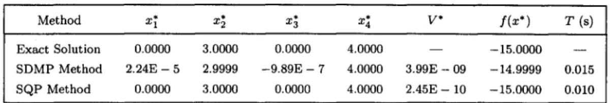
E X A M P L E 3. (See [30].) Minimize: subject to: f ( x ) = X l - x 2 - x 3 - X l X a + x l x 4 + x 2 x 3 - x 2 x 4 , 8 - - X l - - 2 x 2 ~ 0 , 1 2 - 4 X l - X 2 ~ 0 , 12 - 3Xl - 4x2 ~ 0, 8 - - 2X3 - - X4 ~ O , 8 -- X3 -- 2X4 ~ 0, 5 - - X 3 - - X 4 ~ 0, xi > 0, i = 1 , . . . , 4 .

T h e original design space can be decomposed into two decomposed spaces t h a t are spanned by {Xl,X2} and {x3,x4}, respectively. T h e decomposed-space subproblems then become the following. Subproblem 1. f ( x ) = x l - x 2 - x l x 3 + x l x 4 + x 2 x 3 - x 2 x 4 , subject to: 8 - Xl - 2x2 _~ 0~ 1 2 - 4Xl - x2 _> 0, 12 - 3xl - 4x2 _~ 0, x~ >_ 0, i = 1,2. Subproblem 2. f ( x ) = - x 3 - X l X 3 + x l x 4 + x 2 x 3 - x 2 x 4 , subject to: 8 - 2x3 -- x 4 ~ 0, 8 - - X 3 - - 2 X 4 ~ 0 , 5 - - X3 -- X4 >_ 0, xi >_ 0, i = 3, 4.

Further decomposing the spaces into one-dimensional decomposed spaces, the decomposed-space subproblems become Subproblem 1. subject to: f ( x ) = X l - x l x 3 +XlX4, 8 -- Xl -- 2X2 ~ 0, 1 2 - 4Xl - x2 ~ 0, 1 2 - 3Xl - 4x2 ~ 0, Xl ~ 0.

Subproblems 2-4 have forms similar to Subproblem 1. Since only inequality constraints are presented in this problem, the cumulative constraint measure (12) can also be applied to this problem. T h e numerical results as compared to the SQP m e t h o d [31] are shown in Table 3.

(11)

Space-Decomposition Multiplier Method

Table 3. Numerical results of Examples 3 as compared to the SQP method.

61

* * * V *

Method x 1 X~ X 3 X 4 f(X*) T (s)

Exact Solution 0.0000 3.0000 0.0000 4.0000 - - -15.0000 - -

SDMP Method 2.24E - 5 2 . 9 9 9 9 -9.89E - 7 4 . 0 0 0 0 3.99E - 09 -14.9999 0.015

SQP Method 0.0000 3.0000 0.0000 4.0000 2 . 4 5 E - 10 -15.0000 0.010

T h e n u m e r i c a l r e s u l t s for all e x a m p l e p r o b l e m s were o b t a i n e d o n a P e n t i u m 150 M h z m a c h i n e w i t h 48 M B of R A M m e m o r y . T h e L a g r a n g i a n c o n d i t i o n for t h e i n n e r loop a n d t h e c o n s t r a i n t c o n d i t i o n for t h e o u t e r loop were set as c1 = 10 - 4 a n d ~2 = 10 - s , respectively. As s h o w n i n T a b l e s 1-3, t h e n u m e r i c a l m i n i m i z a t i o n s o l u t i o n s from t h e S D M P m e t h o d are s i m i l a r t o t h e s o l u t i o n s from t h e S Q P m e t h o d . I n a d d i t i o n , t h e c o n s t r a i n t v i o l a t i o n s a n d t h e efficiency are also e q u i v a l e n t t o t h a t of t h e S Q P m e t h o d .

10. C O N C L U S I O N S

A f u n d a m e n t a l c o n v e r g e n t s p a c e - d e c o m p o s i t i o n m u l t i p l i e r m e t h o d is p r e s e n t e d i n t h i s p a p e r for c o n s t r a i n e d m i n i m i z a t i o n problems. T h i s m e t h o d allows m i n i m i z a t i o n p r o b l e m s t o b e d e c o m - posed i n t o s u b p r o b l e m s t h a t c a n be solved u s i n g zero- or o n e - o r d e r c o n v e r g e n t a l g o r i t h m s . T h e c o n s t r a i n set c a n also be d e c o m p o s e d i n t o p o t e n t i a l c o n s t r a i n t set a n d n o n p o t e n t i a l c o n s t r a i n t set. I t is s h o w n t h a t a n y c o n s t r a i n t n o t in t h e p o t e n t i a l c o n s t r a i n t set c a n be t e m p o r a r i l y r e m o v e d from t h e c o n s t r a i n t set in t h e d e c o m p o s e d space. N u m e r i c a l r e s u l t s show t h a t t h e n e w m u l t i p l i e r m e t h o d c a n p e r f o r m well w i t h t h e p o t e n t i a l c o n s t r a i n t strategy.

R E F E R E N C E S

1. M.R. Hestenes, Multiplier and gradient methods, Journal of Optimization Theory and Applications 4 (5), 303-320, (1969).

2. M.J.D. Powell, A method for nonlinear constraints in minimization problems, In Optimization, (Edited by R. Fletcher), Academic Press, New York, (1972).

3. S. Zhang and A.G. Constantinides, Lagrange programming neural networks, IEEE Transactions on Circuits

and Systems, II: Analog and Digital Signal Processing 39 (7), 441-452, (1992).

4. C.Y. Maa and M.A. Shanblatt, A two-phase optimization neural network, IEEE Transactions on Neural

Networks 3 (6), 1003-1009, (1992).

5. Z.L. Stan, Improving convergence and solution quality of Hopfield-type neural networks with augmented Lagraage multipliers, IEEE Transactions on Neural Networks 7 (6), 1507-1516, (1996).

6. B.K. Kannan and S.N. Kramer, An augmented Lagrange multiplier based method for mixed integer discrete continuous optimization and its applications to mechanical design, ASME Journal of Mechanical Design 116, 405-411, (1994).

7. A. Ben-Tal and M. Zibulevsky, Penalty/barrier multiplier methods for convex programming problems, SIAM

Journal on Optimization 7 (2), 347-366, (1997).

8. C.H. Tseng and J.S. Arora, On implementation of computational algorithms for optimal design, 1: Prelim- inaxy investigation, 2: Extensive numerical investigation, International Journal for Numerical Methods in

Engineering 26, 1365-1402, (1988).

9. V.H. Nguyen and J.J. Strodiot, On the convergence rate for a penalty function method of exponential type,

Journal of Optimization Theory and Applications 27 (4), 495-508, (1979).

10. P. Tseng and D.P. Bertsekas, On the convergence of the exponential multiplier method for convex program- ming, Mathematical Programming 60, 1-19, (1993).

11. C.S. Liu and C.H. Tseng, Space-decomposition minimization method for large-scale minimization problems,

Computers Math. Applic. 37 (7), 73-88, (1999).

12. C.S. Liu and C.H. Tseng, Parallel synchronous and asynchronous space-decomposition algorithms for large- scale minimization problems, Computational Optimization and Applications, (1998).

13. W. Xicheng, D. Kennedy and F.W. Williams, A two-level decomposition method for shape optimization of structures, International Journal for Numerical Methods in Engineering 40, 75-88, (1997).

14. U. Kirsch, Two-level optimization of prestressed structures, Engineering Structures 19 (4), 309-317, (1997). 15. G. Thierauf and J. Cai, Parallel evolution strategy for solving structural optimization, Engineering Structures

19 (4), 318-324, (1997).

16. J. Sobieszczanski-Sobieski, B.B. James and M.F. Riley, Structural sizing by generalized, multilevel optimiza- tion, AIAA Journal 25 (1), 139-145, (1987).

(12)

62 C.-S. LIU AND C.-H. TSENG

17. C.S. Liu and C.H. Tseng, Two-level learning algorithm for multilayer neural networks, In 10 th IEEE Inter-

national Conference on Tools w~th Artificial Intelligence, Taipei, Taiwan, November 10-12, 1998, pp. 97-102,

(1998).

18. V.M. Kibardin, Decomposition into functions in the minimization problem, Automation and Remote Control 40 (1), 1311-1323, (1980).

19. K. Mouallif, V.H. Nguyen and J.-J. Strodiot, A perturbed parallel decomposition method for a class of nonsmooth convex minimization problems, SIAM Journal on Control and Optimization 29 (4), 829-847, (1991).

20. A. Bouaricha and J.J. Mord, Impact of partial separability on large-scale optimization, Computational Opti-

mization and Applications 7 (1), 27-40, (1997).

21. M.C. Ferris and O.L. Mangasarian, Parallel variable distribution, SIAM Journal on Optimization 4 (4), 815-832, (1994).

22. M.V. Solodov, New inexact parallel variable distribution algorithms, Computational Optimization and Ap-

plications 7, 165--182, (1997).

23. M. Fuknshima, Parallel variable transformation in unconstrained optimization, SIAM Journal on Optimiza-

tion 8, 658-672, (1998).

24. J.T. Betts, A gradient projection-multiplier method for nonlinear programming, Journal of Optimization

Theory and Applications 24 (4), 523-548, (1978).

25. J.S. Arora, Introduction to Optimum Design, pp. 355-356, pp. 387-392, McGraw-Hill, New York, (1989). 26. P. Hajela, C.L. Bloebaum and J. Sobieszczanski-Sobieski, Application of global sensitivity equations in mul-

tidisciplinary aircraft synthesis, AIAA Journal 27 (12), 1002-1010, (1990).

27. S.S. Rao, Engineering Optimization: Theory and Practice, 3 rd Edition, pp. 521-530, pp. 630-635, John Wiley • Sons, New York, (1996).

28. R.T. Rockafellar, The multiplier method of Hestenes and Powell applied to convex programming, Journal of

Optimization Theory and Applications 12 (6), 555-562, (1973).

29. H.M. Adelman and l:t.T. Haftka, Sensitivity anslysis of discrete structural systems, AIAA Journal 24 (5), 823-832, (1986).

30. W. Hock and K. Schittkowski, Lecture Notes in Economics and Mathematical Systems 187, Springer, Berlin, (1980).

31. C.H. Tseng, W.C. Liao and T.C. Yang, MOST 1.1 manual, Tech. Report AODL-9-96-01, Department of Mechanical Engineering, National Chiao Tung University, Hsinchu, Talwan, R.O.C, (1996).