Cancer as A Mini-Evolutionary Process

Department of Mathematics, National Tsing-Hua University January 6, 2010y ,

Cancer as a mini-evolutionary process.

Yoh Iwasa

Evolution: slow change of organisms

mutation:

i

k

f

d

i

mistake of reproduction

natural selection:

mutant with a higher survival

and a faster reproductive rate

and a faster reproductive rate

will replace the old type.

Colon cancer arises in a crypt

Colon cancer arises in a crypt

Apoptosis

on top of crypt A crypt consists

of 1000-4000 cells.

36 hours

A small number of stem cells replenishes the whole crypt.

7

Tumorigenesis includes multiple steps of

t ti

f t

ll

l

f

mutations of stem cells:

z

loss of tumor suppressors

z

oncogenes

g

z

angiogenesis (induction of blood vessels)

metastasis

z

metastasis

z

etc.

Carcinogenesis is an Evolutionary Process

Carcinogenesis is an Evolutionary Process.

(1) Chromosomal Instability

(2) Tissue structure

(2) Tissue structure

Tumor Suppressors

p53

_{Tumor Suppressors}

Rb

prevents cell division

d

i

APC

and causes apoptosis,

if

thi

i

Loss of Both Copies of a Tumor Suppressor Gene is

is

the First Step toward Cancer.

+ + / TSG TSG + /− TSG− /− u + p₀ 2u TSG TSG SG Cancer initiation E t i Escape apoptosis

Chromosomal Instability (CIN)

Chromosomal Instability (CIN)

Normal cells

Normal cells

C

Ch

l I t bilit

Can Chromosomal Instability

Effect of Chromosomal Instability (CIN)y ( )

+ + /

TSG TSG + /− TSG− /− Cancer initiation_{ith t CIN}

u + p₀ 2u TSG TSG TSG _{without CIN} 2 2 Cancer initiation 2n_cu 2n_cu

fast

+/− TSG +/+

TSG Cancer initiation_{with CIN}

p

fast

CIN _2u CIN − TSG CIN Loss Of Heterozygosity Heterozygosity

Fixation of mutant

1 0 1.0 0 ₁ fraction 0.0 0.0 cell generations 1 O(N) 1 Nuρ

( )

r >>

Moran Process

1 Select a cell for reproduction 1. Select a cell for reproduction 2. Cell division

4 Add the new cell 4. Add the new cell

Fixation probability

ρ

( )

r

Fixation probability

N l N ll

ρ

( )

1.0 1.0 N: large N: small 1.0 1/N 0.0 0 1 _r fitness 0.0 0 1 _r fitness fitness fitness

Deleterious mutations can be fixed,,

if N is small.

Fixation of an

intermediate

mutant

1 0 1.0 0 1 2 0 0 0.0 cell generations

T

li

Tunneling:

The Second Mutation Spreads without the Fixation of p the First One

1.0

0 2

1

0.0

explicit formula for tunneling rate

⎡ ⎤

explicit formula for tunneling rate

R_tunnel ≈ Nu₁ − 1− r( )+ 1− r( ) 2 + 2 1+ r( )ru₂ρ( )a 1+ r − ρ( )r ⎡ ⎣ ⎢ ⎢ ⎤ ⎦ ⎥ ⎥ 1+ r ⎣ ⎢ ⎦ ⎥ +

deleterious mutation

Nu₁ ru2 1− r ρ( )a − ρ( )r ⎡ ⎣ ⎢ ⎤ _⎦ ⎥ + if 1− r >> 2 u₂ρ( )a ⎧ ⎪ ⎪

deleterious mutation

≈ ⎣ ⎦₊ N ⎡ _⎢ ( ) 1 ⎤ _⎥ if 1 2 ( ) ⎨ ⎪ ⎪ ⎪ Nu₁ u₂ρ( )a − N ⎣ ⎢ _⎦ ⎥ + if 1− r << 2 u₂ρ( )a ⎩ ⎪

neutral mutation

neutral mutation

Intermediate mutant is deleterious

Fixation probability of Type 2 mutant 0.008 0 006 X 0.004 2 0.006 tunneling 1 t 0.002 1-step process 0.0 0 20 40 60 N fixation of type 1 2-step process N 2-step process

Small compartment: 2-step evolution

Intermediate mutant is neutral

Fixation probability of Type 2 mutant 0.03 li 0.02 X₂ tunneling 1-step process 0.01 fixation of type 1 0.0 0 20 40 60 80 N 2-step process N

Small compartment: 2-step evolution

) ( ) ( 2Nu u + p₀ ρ a ) ( ) (u p₀ a N + ρ 2u TSG + /+ TSG + /− TSG − /− 0 X X₁ X₂ ) (r Nu_cρ ) (r Nu_cρ ) ( 1 2 p ar r r u Nu _c ρ − 1 r (ar) rp Nu_c ρ − 2u TSG + /+ TSG + /− fast TSG − /− 0 Y Y₁ Y2 TSG + /+ TSG + / TSG /

CIN CIN CIN

) ( 2Nu pρ a

r

<1 ) ( 1 2 p ar r r Nuu_c ρ −

C

Ch

l I t bilit

Can Chromosomal Instability

Chromosomal Instabilityy

/+ 2u / u + p0 / Cancer initiation

+ /

TSG TSG + /− TSG− /− Cancer initiation_{without CIN}

p₀

2n_cu 2n_cu

+/−

TSG

+/+

TSG Cancer initiation_{with CIN}

p

fast

CIN _2u CIN − TSG CIN Loss Of H i p

CIN _2u CIN CIN

Heterozygosity

D

th Ti

St

t

Does the Tissue Structure

Change the

Cancer Risk?

Colon cancer arises in a crypt

Colon cancer arises in a crypt

Apoptosis

on top of crypt A crypt consists

of 1000-4000 cells.

36 hours

A small number of stem cells replenishes the whole crypt.

7

Small Compartments Large Compartments Mutants with

Small Compartments Large Compartments

(gate-keeper) Mutants with higher fitness (gate keeper) Mutants with lower fitness (care-taker) S ll Small compartments

reduce the risk of mutants with higher fitness, but enhance the risk of CIN.

Moran Process

1 Select a cell for reproduction 1. Select a cell for reproduction 2. Cell division

4 Add the new cell 4. Add the new cell

1. Select a cell for reproduction

2. Cell division

Linear Process

3. Shift the others division

No Somatic Selection

CIN is important

(1) Compartmentalization

(1) Compartmentalization

(2) Stem cells/non-stem cells

Somatic Selection is Suppressed

Somatic Selection is Suppressed

Risk via High Fitness Mutants is Reduced Risk via High Fitness Mutants is Reduced Risk via Low Fitness Mutants is Enhanced

Dynamics of Chronic Myeloid

y

y

Leukemia (CML)

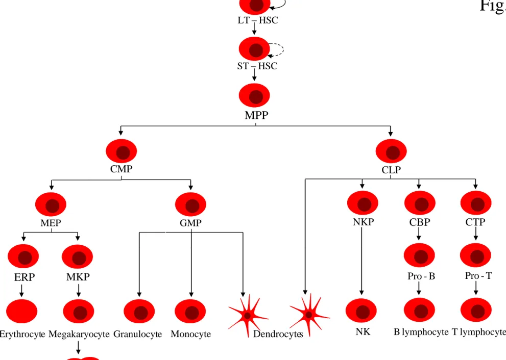
Fig. 1 HSC LT− HSC ST− MPP CMP CLP MEP GMP NKP CBP CTP

ERP MKP Pro-B Pro-T

s Dendrocyte

e

Erythrocyt Megakaryocyte Granulocyte Monocyte NK Blymphocyte Tlymphocyte

I

i ib

i

Imanitib

is a very

effective drug.

g

Under treatment

cancer cells

cancer cells

decrease

in two phases

After the stop of treatment, the number of cancer cells

quickly increases and exceeds the original level.g

Why?

Why?

Resurgence

Resistant Resistant

normal cells

regulated at a constant level stem cells

transition is accompanied

b i i b

progenitor cells

by expansion in number (finite time cell divisions)

differentiated cells differentiated cells

observed cell number

terminally differentiated cells

leukemic cells normal cells stem cells stem cells progenitor cells progenitor cells differentiated cells differentiated cells differentiated cells differentiated cells terminally differentiated cells terminally differentiated cells without treatment

leukemic cells normal cells stem cells stem cells progenitor cells progenitor cells differentiated cells differentiated cells differentiated cells differentiated cells terminally differentiated cells terminally differentiated cells with treatment

P l i D i M d l Population Dynamic Model

? x ₀ =

[

λ( )x₀ − d₀

]

x₀ y ?₀ = r

[

_y(1− u)− d₀

]

y₀ ? x ₁ = a_xx₀ − d₁x₁ y ?1 = ayy0 − d1y1 ? x ₂₂ = b_xxx₁₁ − d₂₂x₂₂ y ?₂ = b_yy₁ − d₂y₂ ? x ₃ = c_xx₂ − d₃x₃ y_{2 y}y_{1 2}y₂ ? y ₃ = c_yy₂ − d₃y₃ 3 x 2 3 3 y3 yy2 3y3

Two rates of Two rates of cancer cells decrease decrease correspond to turnover rates of PC and DC d₂ = 0.05 d₁ = 0.008 1 d₂ = 20 days _{1 =125 days} d₁ =125 days

After the stop of treatment, the number of cancer cells

quickly increases and exceeds the original level.g

S ll

Stem cells are

leukemic cells resistant tumor normal cells SC SC stem cells PC PC progenitor cells DC DC differentiated cells DC DC differentiated cells TC TC terminally differentiated cells with treatment

Population Dynamic Model ? x ₀₀ =

[

[

λ( )( )x₀₀ − d₀₀

]

]

x₀₀ y ?₀ = r

[

_y(1− u)− d₀

]

y₀ z ?₀ = r( _z − d₀)z₀ + r_yy₀u ? d y₀

[

_y( ) ₀

]

y_{0 0} ( _{z 0}) _{0 y}y₀ ? y a y d y ? d ? x ₁ = a_xx₀ − d₁x₁ y ?1 = ayy0 − d1y1 ? b d ? z ₁ = a_zz₀ − d₁z₁ ? x ₂ = b_xx₁ − d₂x₂ y ?2 = byy1 − d2y2 z ?2 = bzz1 − d2z2 ? x ₃ = c_xx₂ − d₃x₃ y ?3 = cyy2 − d3y3 z ?3 = czz2 − d3z3 i ll resistant cells

Model for the number of resistant cells

h iti ll b h M

when sensitive cell number reaches M

M

lls

the detectable number

M

em ce sensitive cells m ic st e u mutation rate euke m u mutation rate r of l e resistant cells u mbe r time n u

= 1 − exp[ −

R

• p

M −1

∑

]

probability of

_{= 1 exp[}

R

_x

• p

_x x=1

∑

]

resistance

expected number of new mutations

survivorship of one lineage until the detection time

is the expected number of new mutations

R

is the expected number of new mutations

when the number of sensitive cells is .

x

R

_x f₁( )0 =1, f_x( )0 =0 for x =2, 3,...,M−1 R_x = rux 1 d / fx(t)dt ∞

∫

df₁ dt = 2df2 − (r + d) f1 1− d /r

∫

_{0 dfx} dt = r(x −1) fx−1 + d(x +1) fx+1 − (r + d)xfx df r: division rate _df M−1 dt = r(M − 2) fM−2 − (r + d)(M −1) fM−1 d: death rate u: mutation rate the probability th t th iti ll t ti

t

generating function: g g g (ξ, t) = E[ξZ ( t ) | Z (0) = 1] ⇒ g (ξ,0) =ξ g (ξ, t + Δt) = aΔtg (ξ, t)2 + bΔt •1+ (1− (a + b)Δt)g (ξ, t) g(ξ ) g(ξ ) ( ( ) )g(ξ ) ⇔ ∂g ∂t = (a − bg )(1− g ) (ξ 1)(b a)e( a−b )t (ξ b a) ⇔ g (ξ, t)= (ξ −1)(b a)e ( ) − (ξ − b a) (ξ −1)e( a−b )t − (ξ − b a) 1 M M = x exp[(r − d)t] t = 1 r − d log( M x ) 1 b ⎛ ⎜ ⎞ ⎟ 1 b ⎛ ⎜ x ⎞ ⎟ a−b ( ) (r−d) ⎡ ⎢ ⎤ ⎥ p_x = 1− a ⎝ ⎜ ⎠ ⎟ 1− a M⎝ ⎜ ⎠ ⎟ ⎣ ⎢ ⎢ _⎦ ⎥ ⎥

Probability of Resistance

Probability of Resistance

⎡

⎤

P

=1− exp −

MuF

1 d

⎡

⎣

⎢

⎤

⎦

⎥

1

1

− d r

⎣

⎢

⎦

⎥

F = 1− b a 1− (b a)y(a−b) (r−d) dy 0 1

∫

where ( )y 0 d i i i

M : detection size u : mutation rate r, d : division/death rate (sensitive cells) a, b : division/death rate (resistant cells)

Simulation results fit the formula

Simulation results fit the formula.

0.5 0.4 M=104 a− b r− d = 2 P 0.3 0.4 0.3 P d=b=1 u=10−5 r d 0 1 0.2 r_a= 2_{= 3} d = b = 1 u= 10−5 0.1 0.2 0.1 104 2×104 3×104 4×104 5×104 u= 10 1.2 1.4 1.6 1.8 2.0 M (detection size)

r

(division rate)

Slow growth implies higher risk of resistant

Slow growth implies higher risk of resistant

cells

small r higher risk of

small r higher risk of

resistance

longer time until diagnosis longer time until diagnosis

more mutations more cell division

Mean number of Mean number of resistant cells

(conditional to one or (conditional to one or more resist. cells)

Distribution of

i t

t

ll

resistant cell

number

z: large Pr y[ ₁ < Y ≤ y₂]= 1 − 1 z: large Pr y[ ₁ < Y ≤ y₂] Fy₁ ( )1α Fy₂ ( )1α ( )2 ₁ ( )y 1 1 z: small Pr Y[ = y]= (1− b a) 2 αF z1α(1− z)y−1 1− b a( )z ( )y+1 dz 0 1 ∫

Cancer Progression

Cancer Progression

is

is

Somatic Evolution

Somatic Evolution.

Collaborators

zMartin A. Nowak (PED, Harvard Univ)

zFranziska Michor (Sloan-Kettering Cancer Research Inst.)

zFranziska Michor (Sloan Kettering Cancer Research Inst.)

zSteven A Frank (UC Irvine)

zRobert May (University of Oxford)y ( y )

zDominik Wodarz (UC Irvine)

zNatalia L Komarova (UC Irvine)

zBert Vogelstein (Johns Hopkins Univ.)

zChristoph Lengauer (Johns Hopkins Univ.)

zTim. P. Hughes (Inst.Med.Vet.Sci. Adelaide)

zSusan Branford (Inst.Med.Vet.Sci. Adelaide)

zN il P Sh h (UCLA)

zNeil P. Shah (UCLA)

zCharles L. Sawyers (UCLA)

zHi hi H (K h U i i )

Probability of drug resistance

d

b

f

i

i

and number of resistance in CML

Poisson distribution of infected

ll

b

( i l i f

i

)

cell number (viral infection)

Drug resistance requires two mutations

Age distribution for CML incidence

g

Drug resistant virus:

Drug resistant virus:

• HIVHIV

• hepatitis B virus • influenza virus

• simple herpes virussimple herpes virus Pathogenic virus

Pathogenic virus ..

(1) produces enzymes decomposing the drug (2) changes the structure of target molecules (3) interrupt the drug delivery

http://web.uct.ac.za/depts/mmi/stannard/emimages.html http://www.howstuffworks.com/aids2.htm

When virus infection is diagnosed,

what is the probability for resistant

strain(s) already to exist in the host.

Proliferation of Virus

target cell

viral particles from a single infected cell Virus

lti l i f t d

p g

can infect multiple cells.

an infected cell Viral particles

multiple infected cells

: mean number of mutants when the b f i f t d ll i

R

_x

number of infected cells is x

f f f x f_x−1 f_x f_x+1 r r r r R = rux f (t)dt ∞

∫

d d d d R_x = 1− ?g

∫

₀ fx(t)dt f 0( )= 1 f ( )0 = 0 for x = 2 3 M 1 x cells x+1 cells x-1 cells probability of x infected cells at t f₁( )0 = 1, f_x( )0 = 0 for x = 2, 3, ..., M − 1 df₁ dt = (d + r ⋅ e −λ )⋅ 2 ⋅ f₂−{d + r(1−λe−λ)}⋅1⋅ f₁ df x−1 λ(x−k +1) probability of extinction of infected cells df_x dt = r λ( ) (x− k +1)!e −λ_{⋅ k ⋅ f} k + k=1 ∑ (d+ r ⋅ e−λ)⋅ (x +1) ⋅ f_x+1 −{d + r(1−λe−λ)}⋅ x ⋅ f_x df M_∑−2 λ(M−k ) re−λ(1− ?g ) + d = (r + d)?g df_M−1 dt = r λ( ) (M− k)!e −λ_{⋅ k ⋅ f} k k=1 ∑ −{d + r(1−λe−λ)}⋅ (M −1) ⋅ f_M−1

: probability for the lineage of resistant cell

q

p y g

line until the onset of drug use.

q

_x M q = ν i e−ν

(

1− gi

)

∞ ∑ = 1 − e−ν(1− g_x ) q_x i! e

(

1 gx

)

i= 0 ∑ 1 e 1 ⎛ ⎞ M ⎛ ⎞ x g _{b bilit f ti ti} g_x = g 1 r(λ − 1) − d log M x ⎛ ⎝ ⎜ ⎞ ⎠ ⎟ ⎛ ⎝ ⎜ ⎞ ⎠ ⎟ R_x q 1 i 0 g_{x : probability of extinction} of resistant virus time q_x t i 0 M = x exp[{r(λ −1) − d}t] t = 1 (λ 1) d log M ⎛ ⎝ ⎜ ⎞ ⎠ ⎟ dg dt = ae −ν(1− g ) _{+ b − (a + b)g , g (0) = 0} r(λ−1) − d ⎝ ⎠ x

Probability that one or more cells are

infected by drug resistant virus y g

at diagnosis

(1 point mutation is enough for resistance)

M 1

⎡

⎤

(1 point mutation is enough for resistance)

R

q

_x

P

=1−exp−

rux

?

f

x

(t)dt

∞

∫

M−1

∑

⋅(1−exp−

(

ν

(1

−g

_x

)

)

⎡

⎣

⎢

⎤

⎦

⎥

R

_x

q

_x

p

1

−?g

∫

0

f

x

( )

x=1

∑

(

p ( g

(

_x

)

)

⎣

⎢

⎦

⎥

M : population size at diagnosis u : mutation ratep p g

r, d : cell division/mortality (wild type) a, b (resistant strain)

Probability of drug resistance is high

when....,

i P r=1.5 • mutation rate u is high r=5

• infected cell number

r : reproductive

rate of sensitve type

ec ed ce u be at diagnosis M is large P u（mutation t ) 1 5 is large d ti t i rate) P _r=1.5 r=5 • reproductive rate r is small M (cell number)

Risk of drug resistance is high, when.. mutation rate is high

mutation rate is high

population size at diagnosis is large

p p g g

population growth rate of virus is slow

Risk of drug resistance is reduced

b id tif i ti t d t ti d

by identifying patients and starting drug treatment as early as possible.

When leukemic stem cell number reaches

M th ti t i di d CML

Current d l

Symptoms of CML

M, the patient is diagnosed as CML.

M

ls model: Symptoms of CML appear

M

m cel l drug sensitive stem cells ic ste m stem cells u mutation rate u kem i u mutation rate of le u drug resistant stem cells m ber time Nu m

A tissue grows exponentially in development. Mutant cells can be produced in the process

Alternative

Mutant cells can be produced in the process, and some descendent may exist at diagnosis.

interpretation： End of development

M

normal cells cells er of c u mutation rate N umb e mutant cells (later causing N (later causing disease) time

Probability of drug resistance

d

b

f

i

i

and number of resistance in CML

Poisson distribution of infected

ll

b

( i l i f

i

)

cell number (viral infection)

Drug resistance requires two mutations

Age distribution for CML incidence

g

Clinical problems caused by cells

p

y

with two specific mutations.

- Drug resistance

CML cells acquires resistance when it becomes

resistant to two different drugs (Imatinib and Dasatinib)

(L387M/F317I etc.)

- Cancer

Retinobrastoma is caused when both alleles of Retinobrastoma is caused when both alleles of

tumor suppressor gene RB1 in a cell are inactivated during development

Model

r

1

a a₂

Type-0 cell Type-1 cell

1 a Type-2 cell 2 a 1 u u₂

Type 0 cell Type 1 cell

d

Type 2 cell

b₁ b₂

Type-0: Wild type cells Type 0: Wild type cells

Type-1: Cells with one mutation (intermediate state) (intermediate state)

Type-2: Cells with two mutations

( ll d i ll )

Parameters

number of mutants cell division rate cell death rate

mutants _{rate rate}

T 0 ₀

r

d

Type-0 1 u 0

r

d

Type-1 ₁

a

₁

b

₁ u₂ Type-2 ₂

a

₂

b

₂

Model

cell number Type-0 mutation mutation Type-1 Type-2 time yp

Probability that fhe first Type-1 cell that survives is producedwhen there are x Type 0 cells

P

_x

:

is producedwhen there are x Type-0 cells.

P −σR ′

(

1 −σR

)

x−1

∏

− x−1( )σR 1 −σR

(

)

P_x = e σRx ′

(

1− e σRx

)

′ x =1

∏

= e ( )x 1σR_x 1− e σRx

(

)

r

When the total cell number reaches M

Expected number of mutants

produced while there are x Type-0 cells:

ell numbe

R_x ≈ u1

1− d r

ce

Probability the linearge from a newly

x

σ ≈1− b1

formed Type-1can survive:

1

time t

Probability that type 1 cells produce type 2 cell(s)

b f th t t l ll b h th fi l l

before the total cell number reaches the final value

Q

=1−e

−u2y 1( −b1 a1)

Q

_x

=1−e

The number of type 1 cells

m

ber

y

= e

(a1−b1)τx

when total cell number reaches the final value

when cell number reaches the final number

cell nu

m

y

y

= e

:time from the production of a Type 1 cell to the final time

τ

_x

x _xe(r−d)τx + e(a1−b1)τx = M

Type-1 cell to the final time

x

1

τ

x Expected number of mutations

until Type-1 cell number reaches y:

time t

u₂y

Probability that one or more Type-2 cell exist

y

yp

at the final time

P

e

−β( )x−1

(

1 e

−β

)

(

1 e

−u2y 1( −b1 a1)

)

M −1

∑

P

=

e

β( )

(

1

−e

β

)

(

1

−e

2y ( 1 1)

)

x=1

∑

β =σR_x = 1− b( ₁ a₁)(u₁ (1− d r))

where

y = e(a1−b1)τx xe(r−d)τx + e(a1−b1)τx = M τ_x

_{is a solution of}

and

y = e( )

r, a₁, a₂: cell division rate

d b b li

x

d, b₁, b₂: mortality

Parameter dependence

Cells with two or more Cells with two or more

mutations exist more likely

– High mutation rates u1 and u2

– Fast cell division rate a₁ of intermediate mutants

– Large final population size M – Large mortality d

Probability distribution of

y

Type-2 cell number

red line: prediction by

red line: prediction by the formula Pr z[ ₁ < Z < z₂]= Pr κ_z 1 <κZ <κz2

[

]

= L L = L_z 2 − Lz1

Probability of drug resistance

d

b

f

i

i

and number of resistance in CML

Poisson distribution of infected

ll

b

( i l i f

i

)

cell number (viral infection)

Drug resistance requires two mutations

Age distribution for CML incidence

g

Step number

0

1

2

1

p

0

1

2

...

n-1

n

Cancer incidence occurs when n stochastic

events occurs to a patient

Probability of incidence on or before age t ）

( )

Step number of CML incidence date is

close to three

If a single mutation is sufficient for CML, can we have step number three?

Moran process

1 choose a single cell randomly 1. choose a single cell randomly.

2. cell division 4 add one cell 4. add one cell

Diagnosis as CML (or detection) occurs

t t ti l t

at a rate proportional to

the number of CML stem cells...

ells em c e m ic st e euke m u mutation rate r of l e u mbe r

i

i

n u

Diagnosis as CML

Probability for a patient to be judged as

leukemia on or before t

⎛ ⎞ ⎡ ⎤

leukemia on or before t

P t

( )

= 1− 1+ e cx −1 N 1 1 r

(

)

⎛ ⎝ ⎜ ⎞ ⎠ ⎟ −qN c ⎡ ⎣ ⎢ ⎢ ⎤ ⎦ ⎥ ⎥ e −b t−x( ) bdx t

∫

N 1

(

−1 r

)

⎝ ⎠ ⎣ ⎢ _⎦ ⎥ 0 b = Nu 1−1 r

(

)

τ c = r −1

(

)

τ

S b f

Step number from

incidence age distribution can be quite large.