利用多部KINECT建構環車3D行車紀錄器及其應用

國

立

交

通

大

學

多媒體工程研究所

碩 士 論 文

利用多部 KINECT 建構環車 3D 行車紀錄器及其應用

Construction and Applications of a 3D Event Data Recorder

Using Multiple KINECT Devices around a Car

研 究 生：張揚

指導教授：蔡文祥 教授

利用多部 KINECT 建構環車 3D 行車紀錄器及其應用

Construction and Applications of a 3D Event Data Recorder

Using Multiple KINECT Devices around a Car

研 究 生：張揚 Student：Yang Chang

指導教授：蔡文祥 Advisor：Wen-Hsiang Tsai

國 立 交 通 大 學

多 媒 體 工 程 研 究 所

碩 士 論 文

A Thesis

Submitted to Institute of Multimedia Engineering College of Computer Science

National Chiao Tung University in partial Fulfillment of the Requirements

for the Degree of Master

in

Computer Science

June 2013

Hsinchu, Taiwan, Republic of China

i

Construction and Applications of a 3D Event Data

Recorder Using Multiple KINECT Devices around a Car

Student: Yang Chang

Advisor: Wen-Hsiang Tsai

Institute of Multimedia Engineering, College of Computer Science

National Chiao Tung University

ABSTRACT

In this study, a 3D imaging system is constructed for use as an event data recorder by affixing multiple KINECT devices to the body of a vehicle. The position and orientation of each KINECT device is different, and totally the views of the 14 KINECT devices in the system cover the 360o car surround. To speed up the data recording work, two computers are used, each controlling seven KINECT devices.

To implement the proposed system, at first a method for creating a 3D model of around-car objects is proposed. This method is based on the pinhole camera model. The constructed around-car object model can be rendered in the 3D space and seen from specific views.

Secondly, a method for calibration of the relationship between neighboring KINECT devices using any calibration target is proposed, which is based on matching the target in a pair of acquired KINECT images using the iterative closest point (ICP) algorithm. Moreover, the calibration process is speeded up by the use of some learned information.

In addition, a method is proposed for merging the images acquired from multiple KINECT devices around the car. With the relationship parameters acquired during the

ii

calibration process as inputs, the method transforms the coordinates between each pair of neighboring KINECT devices to accomplish the merge work.

Also, a method is proposed for panoramic image creation by stitching multiple color images into a single image. The stitching work is carried out by an automatic stitching algorithm. The created panoramic image can be used as a background in the displayed scene because the 3D image data constructed by the system sometimes are not enough.

Finally, a method for combining 3D images with the 2D panoramic image is proposed. Specifically, the panoramic image is projected onto a spherical shape which, together with the 3D around-car object model, is rendered for inspection of the geometric relation between the nearby object and the background scene.

Good experimental results are also shown, which prove the feasibility of the proposed methods for real applications.

iii

利用多部 KINECT 建構環車 3D 行車紀錄器及其應用

研究生：張揚

指導教授：蔡文祥 博士

國立交通大學多媒體工程研究所

摘要

本研究利用架設在車輛上的多台 KINECT 感測器，來建立三維取像系統，做 行車紀錄器之應用。每台 KINECT 感測器的位置都不盡相同，因此所有使用的 14 台 KINECT 感測器的視野加起來可以涵蓋 360o 的車子週遭範圍。為了在紀錄時加 快速度，本研究使用了兩台電腦，每台控制 7 台 KINECT 感測器。 為達到建構 3D 行車紀錄器的目的，首先，本研究提出一個建立三維環車近 景模型的方法，該法是建立在針孔成像的原理上。所建三維還車近景模型可以借 由三維空間顯像技術，由各個不同的角度觀看。 第二步，本研究提出了一個校正兩台相鄰 KINECT 感測器關係的方法，該法 是利用最近點迭代演算法來進行校正工作，並利用一些預先學習的資訊，來進行 加速。 第三步，本研究提出了一個整合車輛上多台 KINECT 感測器所得資料的方 法，該法是利用校正所得兩台 KIMECT 感測器的相對關係參數，對每對相鄰 KINECT 感測器所得之三維近景模型作座標轉換。 第四步，本研究提出了一個將多張由環車 KINECT 感測器所擷取之彩色影像 連接成一張全景圖的方法，該法是基於一自動接圖演算法。因為室外所得到的深 度資訊是不夠多的，所以本研究將環車彩色影像串接出來的全景圖，作為 3D 行 車紀錄器的背景。 第五步，本研究提出了一個將三維環車近景模型與背景圖整合的方法。該法

iv

是將背景圖投影到球體上，與三維環車近景模型做幾何的對應，因此在近的地方 有三維環車近景模型，而在遠的地方則顯示出背景的部分。

v

CONTENTS

ABSTRACT (in English) ... i

CONTENTS ... iii

LIST OF FIG.S... vi

LIST OF TABLES ... x

Chapter 1

Introduction ... 1

1.1 Background and Motivation ... 1

1.2 Review of Related Works ... 3

1.3 Overview of Proposed Methods ... 5

1.4 Contributions ... 7

1.5 Thesis Organization ... 8

Chapter 2

System Design and Processes ... 9

2.1 Ideas of Proposed System ... 9

2.2 System Configuration ... 10

2.2.1 Hardware Configuration ... 10

2.2.2 Software Configuration ... 13

2.3 System Processes ... 14

2.3.1 Learning Process ... 14

2.3.2 Data Recording and Analysis Process ... 16

Chapter 3

Design of Proposed 3D Around-car Imaging System ... 19

3.1 Idea of Proposed 3D Around-car Imaging System ... 19

3.2 Details of System design ... 21

3.2.1 Front Part ... 21

3.2.2 Right- and Left-side Parts ... 23

3.2.3 Rear Part ... 25

3.3 System Performance Analysis ... 26

3.3.1 Ranges of Camera Views... 26

3.3.2 Imaging Sequence and Speed ... 27

Chapter 4

Construction of 3D Images from KINECT Images ... 29

4.1 Review of Structures of Depth and Color Images Taken by KINECT Devices ... 29

4.2 Construction of 3D Images from KINECT Images ... 30

vi

4.2.2 Ideas of 3D Image Construction and Coordinate Conversion .. 32

4.2.3 Construction Algorithm and Experimental Results ... 34

4.3 Review of a Method for Geometric Correction of 3D Images ... 37

4.3.1 Idea of Geometric Correction ... 37

4.3.2 Correction Algorithm and Experimental Results ... 38

Chapter 5

Modeling of Around-car Objects... 40

5.1 Introduction ... 40

5.2 KINECT Camera Calibration ... 41

5.2.1 Review of Calibration of a Single KINECT ... 41

5.2.2 Transformation of Coordinates ... 42

5.2.3 Review of Iterative Closest Point (ICP) Algorithm ... 43

5.2.4 Calibration by the ICP algorithm Using Speeded-up k-d Tree. 44 5.2.5 Calibration of Relation between Neighboring KINECT Devices ... 46

5.3 Merge 3D Images from Multiple KINECT Devices... 47

5.3.1 Coordinate Mapping between Local and global ... 47

5.3.2 Reduction of Merged Data Using Mesh Structure ... 50

5.3.3 Review of Quadric Error Matrix (QEM) ... 51

5.3.4 Merge Algorithm ... 53

5.4 Experimental Results ... 54

5.5 Object Detection ... 55

5.5.1 Object Detection in Depth Images ... 55

5.5.2 Component Labeling by Region Growing on Depth Images for Object Detection ... 56

Chapter 6

Long-Range View Construction and Display ... 58

6.1 Ideas of Proposed Techniques ... 58

6.2 Automatic Panoramic Image Stitching from Multiple KINECT Images ... 59

6.3 Panoramic Image Stitching ... 61

6.4 Merging 3D image with background image ... 66

6.5 Experimental Results ... 69

Chapter 7

Experimental Results and Discussions ... 72

7.1 Experimental Results ... 72

7.2 Discussions ... 78

Chapter 8

Conclusions and Suggestions for Future Works ... 80

vii

8.2 Suggestions for Future Works ... 81

LIST OF FIGURES

Fig. 1.1 The system used in LightSpace. ... 3

Fig. 1.2 A 3D indoor environment model constructed by [4] from KINECT images. .. 4

Fig. 1.3 Geometrically precise 3D models of a room constructed by [5]. ... 5

Fig. 1.4 Illustration of proposed system with multiple KINECT devices. ... 5

Fig. 1.5 Major tasks of proposed KINECT-based around-car EDR system. ... 6

Fig. 2.1 The structure of a KINECT device. ... 10

Fig. 2.2 The USB extension card (the upper is the expansion and the lower is the base) ... 12

Fig. 2.3 Ferrous boxes for holding KINECT devices. (a) Without a KINECT device. (b) With a KINECT device. ... 12

Fig. 2.4 illustration of the role OpenNI plays. ... 13

Fig. 2.5 The learning process for system calibration. ... 15

Fig. 2.6 The learning process for image stitching. ... 15

Fig. 2.7 Master-slave structure of proposed data recording and analysis process where PC1 is the master computer and PC2 is the slave computer. ... 16

Fig. 2.8 Starting the data recording and analysis process. ... 17

Fig. 2.9 Ending the data recording and analysis process. ... 17

Fig. 3.1 The cameras affixed on the body of the car (a) (b) front part of the car (c) (d) side part of the car (e) (f) rear part of the car (g) (h) the recorder on the mirror... 20

Fig. 3.2 Proposed design of the KINECT-device system affixed on the vehicle and the views of the KINECT devices. ... 22

Fig.3.3 A test for driver’s view. (a) Side view. (b) Front view. ... 23

Fig. 3.4. A car-side iron stand for holding a KINECT device. (a) With a KINECT device. (b) Without a KINECT device. ... 24

Fig. 3.5. Ferrous boxes for holding KINECT devices. (a) With a KINECT device. (b) Without a KINECT device. ... 24

Fig. 3.6 Around-car KINECT devices (a) A front view. (b) A back view. (c) A lateral view. (d) A rear-view mirror. ... 25

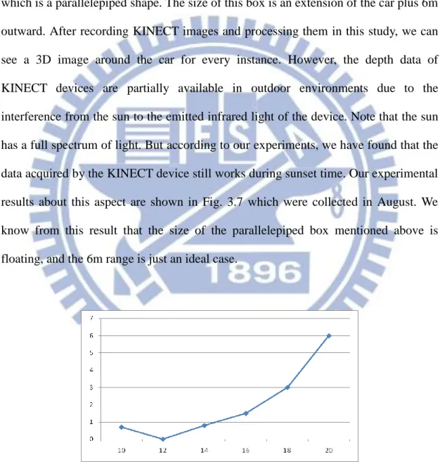
Fig. 3.7 The relationship between the depth image quality and the sun intensity (the x-axis specifies time, the y-axis specifies the available depth range). ... 26

Fig. 4.1 Images acquired with the KINECT device. (a) Color image. (b) Depth image. ... 29

Fig. 4.2 A tree is projected onto the image plane through a pinhole model... 30

viii

Fig. 4.4 The geometry of a pinhole camera as seen from the X2 axis ... 32 Fig. 4.5 A flowchart of 3D image construction algorithm. ... 35 Fig. 4.6 Images acquired by a KINECT device. (a) The depth image. (b) The color image. ... 36 Fig. 4.7 A constructed 3D image. (a) A perspective view of the 3D image. (b) A top view. ... 36 Fig. 4.8 The paraboloid seen from the direction of the Y-axis (i.e., from the top view).

... 37 Fig. 4.9 The 3D image of a wall seen from above. (a) Before correction. (b) After correction. ... 39 Fig. 4.10 The 3D image of another wall seen from the top view. (a) Before correction. (b) After correction. ... 39 Fig. 5.1 The pinhole camera model for calibration of the focal length of the camera. 41 Fig. 5.2 Transformation between two coordinate systems built on KINECT devices affixed on the car. ... 48 Fig. 5.3 The transformations involved in merging three 3D images taken by three neighboring KINECT devices. ... 49 Fig. 5.4 Constructing a mesh on the depth image for each pixel (i, j). ... 50 Fig. 5.5 The contraction of two vertices. (a) Before contraction. (b) After contraction.

... 52 Fig. 5.6 The calibration of two neighboring KINECT devices. (a) Before alignment (b)

After alignment. ... 54 Fig. 5.7 The constructed around-car model. (a) Front view. (b) Rear view. (c) Right side view. (d) Left Side view. ... 54 Fig. 5.8 The constructed around-car model. (a) Front view. (b) Rear view. (c) Right side view. (d) Left Side view. (Continued). ... 55 Fig. 5.9 The object detection result. (a) Original color image. (b) The detected object part in the color image. ... 57 Fig. 6.1 The two images before stitching, where (a) is a slightly left rotated version of (b). ... 60 Fig. 6.2 Stitching result from the two images in Fig. 6.1 using Algorithm 6.1. ... 61 Fig. 6.3 Stitching two images with different values of  and   case 1. (a) and (b) are original images, and (c) is the stitching result with  = 10,  = 0.2.

... 61 Fig. 6.4 Stitching two images with different values of  and   case 2. (a) and (b) are original images, and (c) is the stitching result with  = 0,  = 0.13.

... 62 Fig. 6.5 Stitching result compares with those of Figs. 6.3 and 6.4 with  = 10 and 

ix

= 0.2. ... 63 Fig. 6.6 Two color images acquired from two neighboring KINECT devices where view (a) is a left shift version of view (b), and the essential overlap part (the three cars in the middle) is too small, compared with the parking space in front which has fewer features for matching. ... 64 Fig. 6.7 Two color images with nearby parts cut, where view (a) is a left shift version of view (b). ... 64 Fig. 6.8 Successful stitching result using images in Fig. 6.7 as input. ... 64 Fig. 6.9 Illustration of the stitching method. The neighboring number of images are corresponded to the neighboring position of each KINECT devices. ... 65 Fig. 6.10 The original panoramic image yielded by the panoramic image stitching process illustrated in Fig. 6.8. ... 65 Fig. 6.11 A well-cut version of Fig. 6.9. ... 66 Fig. 6.12 A 3D point in a sphere expressed by polar coordinates. ... 67 Fig. 6.13. A result of polar coordinate transformation applied to a color image acquired by a KINECT device. (a) Seen from the front. (b) Seen from the top with a little slant. (c) Seen right from the top. ... 67 Fig. 6.14 The images before merged. (a) Nearby object in the color image being removed. (b) Rendering of the removed object part into the 3D space. .. 69 Fig. 6.15 The result of merged data. (a) Seen on the front of image. (b) Seen from the top view. ... 69 Fig. 6.16 The result of merged 3D image on to background data which come from stitching by 3 background images... 70 Fig. 6.17 Removal of a near-by car in a panoramic image. (a) Nearby car in the color image being removed. (b) Rendering of the removed car part into the 3D space. ... 70 Fig. 6.18 Different views of result of merging 3D image and 2D panoramic background. (a) A front view. (b) A side view. (c) A top view. ... 71

1

Chapter 1

Introduction

1.1 Background and Motivation

The event data recorder (EDR) of a car, which is similar to an aircraft’s black box, is used by people to record the around-car information “seen” during car driving in a trip, which includes the traffic conditions and possibly car accidents along the way. Such records of “driving history” can be used for judgments of car encountering or collision conditions when legal cases arise. For example, according to a news report, a boy who was nineteen years old drove a jip bump to hit a Rover sport utility vehicle, causing an accident in which only a paralyzed baby survived. The data recorded by the EDR was used to re-build the situation at the car collision instance, finding out that a force equivalent to 42mph was applied in one fifth of a second in the crash. This helped the police to put the defendant’s speed at around 72mph, and it is the first time such technology plays a role in the British court.

The EDR has become more and more popular in recent years. According to the evaluation of National Highway Traffic Safety Administration (NHTSA) of the USA, it is predicted that more than 85 percents of the cars are equipped with EDRs whose capabilities become more and more diversified and powerful due to the market growing trend and the technology advance. Some kinds of high-end EDRs are equipped with wide-angle cameras and provide high-resolution videos, offering capabilities of “seeing wider and clearer.” Moreover, some even better high-end EDRs are designed to include the GPS and dual cameras, the latter being used at the front

2

and rear of the car. This helps people to get a more complete view around the car when one drives to a place for the first time. Furthermore, such intelligent EDRs also help saving power and storage because they start recording only if the view is changing.

In addition, with the advance of 3D vision technology, 3D cameras, 3D phones, 3D movies, 3D TVs, etc. appear one after another in fast speeds. These goods enrich our life in different ways, helping us to “show” the world on various types of displays from 2D ways to 3D ones. These 3D goods inspired us to create a 3D EDR. In this study, we try to build a 3D EDR system with multiple KINECT devices for use on a car to record around-car scenes from different views, so that complete 3D information around the car can be constructed.

Furthermore, when a car accident occurs, the proposed 3D EDR system can help re-building the scene at the accident moment as a 3D version, called a 3D scene. Afterwards, we can browse the 3D scenes in sequence. In this way, we can see the scene just like you were there and holding a camera inside a car. For example, to see how a car bumps onto another, we can turn the 3D scene to the lateral side to check the situation between the two cars at critical moments, or to see the entire course of the event. This helps us to clarify the car-accident responsibility easier than using the record of a traditional “2D” EDR.

Furthermore, the 3D EDR is a tool useful not only for protecting people’s right in car accidents, but also for recording journeys by car driving in the outdoor environment. By the use of the recorded information, people may look back at beautiful scenes, check the shapes of luxury cars driven around, view gorgeous ladies passing by, and so on, all in 3D ways, to enrich our “life of technology!” In this study, we try to design a 3D EDR using around-car KINECT devices and develop techniques to deliver 3D information for this goal.

3

1.2 Review of Related Works

About researches related to 3D device systems, Wilson and Benko, et al [1] proposed an idea of LightSpace created by the research team of Microsoft, and proposed accordingly a smart image display system for use in the office, for which they used three depth sensors and three projector sets installed on the ceiling (as shown in Fig.1.1). Special touch screens or monitors were not used. The depth image which is acquired by the depth camera is transformed into the real-world coordinate system after calibrating each depth camera of the system, so that they could interact with the user in ways such as moving an image from the table to the white board with a user’s hand sign. That means he/she can use a hand to control many complex instructions implemented by integration of the projector and depth cameras in a usual way.

Fig. 1.1 The system used in LightSpace.

Some other systems using different devices for building 3D models have also been proposed. Biber, et al. [2] proposed a robot equipped with a laser distance meter

4

and an omni-camera to get depth information of the real-world environment, extract the information of walls by using the laser distance meter to solve the SLAM problem, and mix up multi-size textures to hide the seams between images. Henry et al. [3] used color and depth images acquired by the KINECT device to propose a method for building a complete 3D mapping system by combining visual features.

About other applications using the KINECT device, a team of the MIT, the University of Washington, and the Intel Lab. at Seattle [4] put KINECT devices on a light aircraft to build a multi-view integrated 3D model of an environment. An example is shown in Fig 1.2. In their method, the feature points in the images acquired by the KINECT devices were extracted and a so-called RGBD-SLAM algorithm was used to achieve their goal of environment modeling.

Fig. 1.2 A 3D indoor environment model constructed by [4] from KINECT images.

In seeking a method for building 3D environment models, Sharam Izadi, et al. [5] proposed the concept of KINECT fusion and designed accordingly a system that takes live data from a moving KINECT device and creates high-quality and geometrically accurate 3D models in realtime. An example of their result is shown in Fig. 1.3. They tracked the previous frame and the current frame to compute a rigid 6DOF transform that closely aligns the currently-oriented points with those of the previous frame,

5

using a novel GPU implementation of the ICP algorithm.

Fig. 1.3 Geometrically precise 3D models of a room constructed by [5].

1.3 Overview of Proposed Methods

In this study, we use KINECT devices around the car to build our 3D EDR system. The concept of this idea is illustrated in Fig. 1.4.

Fig. 1.4 Illustration of proposed system with multiple KINECT devices.

As shown in Fig. 1.5, before acquiring data by the KINECT devices, we measure manually roughly the geometric relation between every two neighboring KINECT devices. Afterwards, we develop a method for finding more precise inter-KINECT relations based on an ICP algorithm, using the hand-measured data as initial values

6

for iterations conducted by the algorithm.

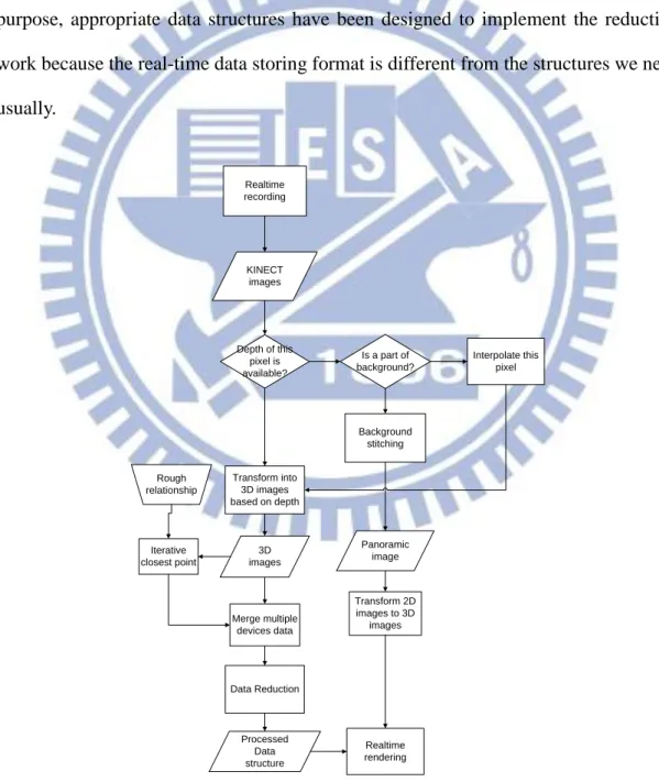
Then, we use a method of coordinate conversion similar to that described in [1] to transform each pixel of the depth image into the real-world coordinate system to construct a 3D image. In the process, a cluster of points are taken to correspond to a single real point existing in the real world. Because the number of points obtained from the KINECT device is pretty large, it is important to reduce the amount of data while keeping the shape of each object good enough without deformations. For this purpose, appropriate data structures have been designed to implement the reduction work because the real-time data storing format is different from the structures we need usually. Realtime recording KINECT images Depth of this pixel is available? Is a part of background? Transform into 3D images based on depth Background stitching Interpolate this pixel Data Reduction Processed Data structure Panoramic image Realtime rendering Transform 2D images to 3D images Iterative closest point 3D images Rough relationship Merge multiple devices data

7

Because of the restriction of the range of KINECT devices, depth data out of 6m are notavailable, but we still want to see some beautiful scene at far distances when we are driving. To satisfy this desire, the long-range views of the surrounding scene provided by the color images are stitched in this study to produce a panoramic image automatically. Furthermore, this panoramic image is attached to a part of a sphere for the purpose of fitting the nearby data obtained from the KINECT devices.

Finally, we can browse the generated 3D images and panoramic views in a form like video from both near and far views, just like browsing a Google Street View in a 3D version. At every instant of the generated video sequence, we can see the 3D objects around us and the scenes at far distance just as if we are standing on the street (but in fact we are standing inside a sphere).

1.4 Contributions

Some contributions of this study are listed in the following.

1. Constructing 3D images by color and depth images acquired with KINECT devices

2. Constructing 3D images for a subset of the KINECT devices and combining them into a single 3D image for each of some specific views (front, lateral, rear, etc.).

3. Constructing a complete around-car 3D image without blind spots from the 3D images corresponding to all the KINECT devices respectively on the car. 4. Combining the long-range color-image views into a mosaic panoramic image

for use as the far-view background image.

5. Providing a realtime browsing system with a series of offline processes for users’ browsing of the panoramic background image.

8

6. Combining near objects and far views around the car to construct 3D images like street views for each time instant for the user to browse.

1.5 Thesis Organization

The remainder of this thesis is organized as follows. In Chapter 2, we introduce the configuration of the proposed system and the system processes in detail. In Chapter 3, we present the design of the proposed 3D around-car imaging system. In Chapter 4, a method for constructing 3D images is described. In Chapter 5, we introduce the proposed method for modeling around-car objects, including calibration and merging multiple KINECT devices. In Chapter 6, the proposed method for browsing a 3D image including integrated long-range views and nearby objects is described. In Chapter 7, experimental results and discussions are presented. Finally, conclusions and some suggestions for future works are given in Chapter 8.

9

Chapter 2

System Design and Processes

2.1 Ideas of Proposed System

In order to build a complete panoramic view around the car, we affix KINECT devices with different orientations to the car body at different locations. We try to consider the use of the minimal number of KINECT devices to cover the entire car body with a 360-degree surround. With the horizontal angle of a KINECT device being 57 degrees, the minimal number of KINECT devices required to accomplish a complete covering of 360o would be 7, but our final design of the 3D around-car system uses 14 KINECT devices as mentioned in Chapter 1. The reason and more details of the design will be described in Chapter 3.

With the 14 KINECT devices, we can acquire depth and color images through universal serial buses (USBs). Since each KINECT device needs one distinct USB controller, we need 14 USB controllers for the proposed system. In turn, we need a special computer with at least 14 USB controllers. But such a computer is not available commercially. Therefore, we insert a USB extension card onto the mother board of a common desk-top computer for use in this study. But the computing speed becomes so slow that we decided to use two computers to build our system, with each computer containing seven USB controllers. Analysis of the resulting processing speed will be described in Chapter 3.

In Section 2.2, we will describe the configuration of the proposed system, including the hardware and the software. The processes conducted by the proposed

10

system, which include a learning process and a data recording and analysis process, will be described in Section 2.3.

2.2 System Configuration

To build the proposed 3D imaging system on the car, we affix 14 KINECT devices on the car as mentioned before. Color and depth images are acquired with the KINECT devices via the OpenNI which is an open source software for use as the device driver. In Section 2.2.1 we will review the functions of the KINECT device, and describe how and where we affix the 14 KINECT devices on the car. In Section 2.2.2, we will introduce system development environment for this study, and the functionality of each component in the system.

2.2.1 Hardware Configuration

At first, we review the structure of the KINECT device as shown in Fig. 2.1. Inside a sensor case, a KINECT device contains an infrared (IR) emitter, an RGB camera, an IR depth sensor, and a tilt motor to control the tilting angle of the KINECT device.

11

The functions of the components of the KINECT device are explained below. 1. An infrared (IR) emitter and an IR depth sensor The IR emitter emits light

to objects in the environment, and the IR depth sensor reads the reflected light from the objects to compute the distances between the objects and the KINECT device by converting the times of flight of the reflected light rays into depth values.

2. An RGB camera  The camera in the KINECT device senses image data of three color channels R, G, and B.

3. An accelerometer  The accelerometer is conFig.d for sensing a 2G range (G is a unit of acceleration due to gravity), by which, we can know the current operational condition of the tilter (i.e., the tilt motor).

4. A multi-array microphone  This device contains four microphones which may be used to record the sound and know the direction of the sound.

Some more specifications of the KINECT device are listed in Table 2.1. Especially, the view angle, the tilt range of the device, and the range of the sensed depth values are important for our design of the proposed system. We will discuss these parameters in more detail later in Chapter 3. Furthermore, some specifications of the desktop computer used in this study are listed in Table 2.2.

Table 2.1 Specifications of the KINECT device.

Horizontal viewing angle 57 degrees

Vertical viewing angle 43 degrees

Tilt range of the device ±27 degrees Range of the depth sensor 1.2-3.5 meters

Resolution of color images 640 x 480

12

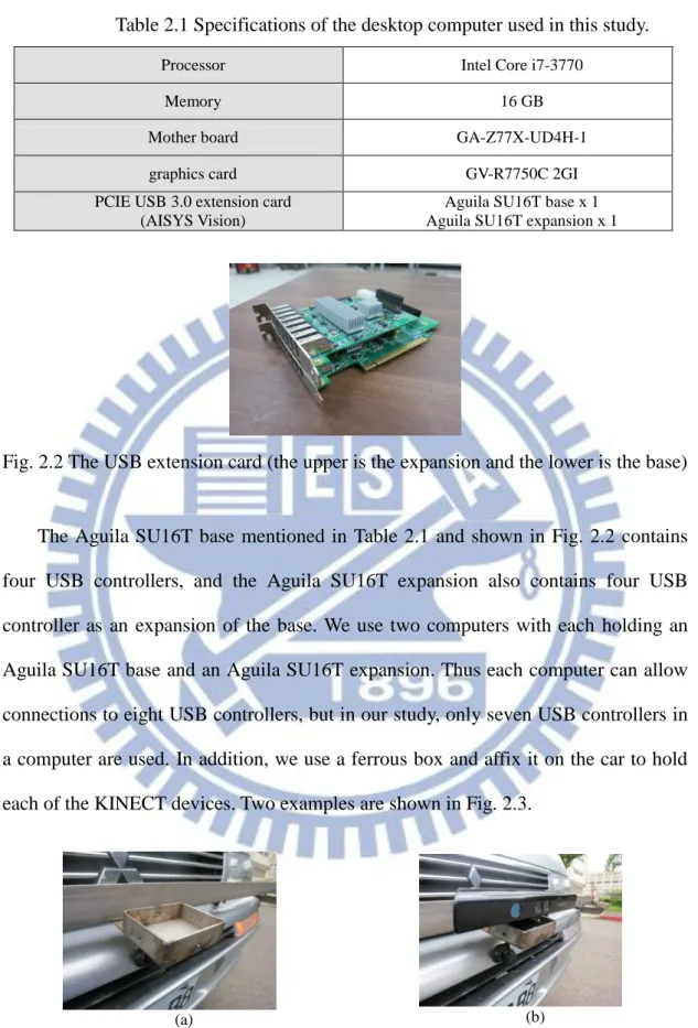
Table 2.1 Specifications of the desktop computer used in this study.

Processor Intel Core i7-3770

Memory 16 GB

Mother board GA-Z77X-UD4H-1

graphics card GV-R7750C 2GI

PCIE USB 3.0 extension card (AISYS Vision)

Aguila SU16T base x 1 Aguila SU16T expansion x 1

Fig. 2.2 The USB extension card (the upper is the expansion and the lower is the base)

The Aguila SU16T base mentioned in Table 2.1 and shown in Fig. 2.2 contains four USB controllers, and the Aguila SU16T expansion also contains four USB controller as an expansion of the base. We use two computers with each holding an Aguila SU16T base and an Aguila SU16T expansion. Thus each computer can allow connections to eight USB controllers, but in our study, only seven USB controllers in a computer are used. In addition, we use a ferrous box and affix it on the car to hold each of the KINECT devices. Two examples are shown in Fig. 2.3.

(a) (b)

Fig. 2.3 Ferrous boxes for holding KINECT devices. (a) Without a KINECT device. (b) With a KINECT device.

13

2.2.2 Software Configuration

About the software configuration, firstly we review the OpenNI which is an open source software for development of 3D sensing middleware libraries and applications as shown in Fig.2.4. It provides a tool for getting depth and color images from KINECT devices, or in other words, it provides an interface to communicate with the hardware and the computer.

Fig. 2.4 illustration of the role OpenNI plays.

Secondly, the OpenGL is an application programming interface (API) for generating 2D and 3D images. This API is typically used to interact with a GPU to achieve hardware-accelerated rendering. In our case, the OpenGL is a tool for rendering 3D data which are obtained from transforming the color and depth images. The details will be described later.

Finally, we use the Visual Studio 2010 as a development environment for integrating multiple kinds of libraries, such as OpenNI and OpenCV. Therefore, we can write programs using the C and C++ languages and the libraries to conduct works of image processing, rendering, …, etc. on this software platform.

14

2.3 System Processes

2.3.1 Learning Process

Before the data recording process, a learning process is necessary. We divide the learning process into two parts as follows.

The first part is the process for system calibration, including the calibrations of the KINECT devices and some system parameters. The first task to be done in this process is to find out the height of each KINECT device with respect to the road in the 3D image. For this, we have to transform the depth and color images acquired by a KINECT device into a 3D image at first. Then, we find the desired height by a try-and-error manner using the 3D image; when an appropriate height parameter is found, we can use it for next steps.

Secondly, we have to calibrate the geometric relation between every two neighboring KINECT devices. For this, we use a box with a simple shape as the calibration target, and take the previous result, the height of each KINECT device, to find the calibration target out in precise. The result of this process is the relative angle between every two KINECT devices, which can be used in the data recording and analysis process. A flowchart of this part of the learning process is shown in Fig. 2.5, and the detail of calibration is described in Chapter 5.

The second part is the process for stitching of multiple images to construct a long-range panoramic view. In this processing, at first we want to learn a threshold value to separate far-view contents from near-view ones in each color image which is taken by the KINECT device. The work is completed by try-and-errors. The resulting set of far views can then be combined together to get a panoramic view by a stitching process which will mentioned in more detail in Chapter 6. A flow chart of this part of

15

the learning process is shown in Fig. 2.6.

Conversion process Threshold of height Depth images 3D images Learning process Result Calibration process

Fig. 2.5 The learning process for system calibration.

Stitching process Color images Learning process Input value Resulting set

16

2.3.2 Data Recording and Analysis Process

In the data recording and analysis process, two computers are in use as the controllers of the 14 KINECT devices and are connected by a cable. They are of a master-slave structure, as shown in Fig. 2.7. The software implementation is based on a client-server architecture which we use a windows socket to conduct the inter-computer communication. Start Initialization of PC 1 Initialization of PC2 Ready for recording Ready for recording User instruction (PC1) PC1 recording PC2 recording

Fig. 2.7 Master-slave structure of proposed data recording and analysis process where PC1 is the master computer and PC2 is the slave computer.

At the beginning of the data recording and analysis process, as shown in Fig. 2.8, at the client side, the master receives an instruction from the user, and then sends a request to the slave at the server side for recording. The slave starts the recording process and returns a reply to the master after getting the request. While receiving a reply from the slave at the server side, the master starts to run the recording process,

17

too. All the communications are implemented by multi-thread, because we have to communicate two devices and record at the same time. The ending of the data recording and analysis process is shown in Fig. 2.9.

Client(master) Server(slave) 2. Request

1. instruction

4. Reply

5. recording 3. recording

Fig. 2.8 Starting the data recording and analysis process.

Client(master) Server(slave) 2. stop request

1. wait the stop pattern

4. stop reply

5. stop recording 3. stop recording

Fig. 2.9 Ending the data recording and analysis process.

Furthermore, a series of tasks are conducted in the data recording and analysis process as described in Section 1.3, including (1) transforming color and depth images acquired by each KINECT device at each time instant into a 3D image; (2) stitching all the color images into a panoramic color background image; (3) extracting nearby 3D objects from the 3D image corresponding to each KINECT device; (4) merging the extracted 3D objects into the panoramic color background image; and (5) allowing

18

the user to browse the merging result from any viewpoint and display the corresponding partial view.

19

Chapter 3

Design of Proposed 3D Around-car

Imaging System

3.1 Idea of Proposed 3D Around-car

Imaging System

When constructing a 3D EDR, it is important to let the EDR “see” the view around the car with no blind spot. It is obviously not enough to use only one KINECT device whose horizontal angle range is 57 degrees only. Instead, we have to affix multiple KINECT devices around the car. In addition, the way of design for this system is different for each distinct part of a car. Before starting the description of the proposed system design, we give a brief review of the design of a car model with multiple cameras produced by Luxgen Motor Co. Ltd.

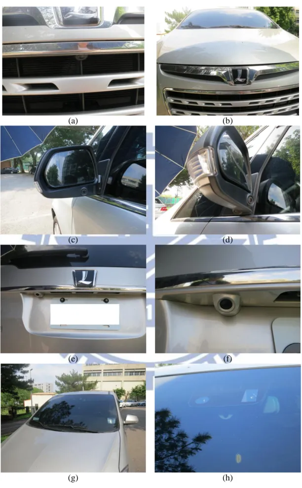
Luxgen has released a new car equipped with six RGB cameras around the car body. They are called “eagle views.” A camera is affixed to the front of the car, and another to the rear. The remaining four cameras are affixed below the side mirrors, with each side equipped with two cameras, one camera facing to the rear of the car, and the other is facing askew to the rear as shown in Fig. 3.1.

20

(a) (b)

(c) (d)

(e) (f)

(g) (h)

Fig. 3.1 The cameras affixed on the body of the car (a) (b) front part of the car (c) (d) side part of the car (e) (f) rear part of the car (g) (h) the recorder on the mirror.

21

This design inspired us, because we can affix cameras on the side mirror. With these cameras, we can seethe around-car view like through the window of the car. If someone gets close to the car near the window, it would be found by the nearby KINECT device.

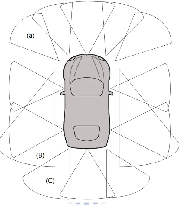
About the coverage of the front view of the car, Luxgen uses only one camera to cover the front view, because the camera is of the fisheye type which yields a wider view than from a normal projective camera. The overlapping portion of the front view and the side view is narrow, and so there exist four bind spots on the corner. To improve it, we use four additional KINECT devices to cover the corner views in our design. Specifically, to cover the front-left corner, a KINECT device with its view covering the portion of (a) as shown in Fig. 3.2 is deployed. A second KINECT device is used to cover the right symmetric portion in the front. For the rear-left corner, a third KINECT device with its view covering the portion of (c) is deployed. And the fourth KINECT device is used to cover the right symmetric portion in the rear.

About the other deployed KINECT devices, we affix three KINECT devices for the front view, four for each side view, and three for the rear view. In addition, we affix a KINECT device on each of the two side mirrors which looks backward to cover the view portion of (B) as shown Fig. 3.2. More details will be described in Section 3.3.

3.2 Details of System design

3.2.1 Front Part

In this section we will focus the part of our design which is related to the driver’s views. Specifically, we will affix KINECT devices to proper car body parts to cover “blind spots” that the driver cannot notice during driving, for example, the part of the

22

front view which is lower than the height of the engine hood.

Fig. 3.2 Proposed design of the KINECT-device system affixed on the vehicle and the views of the KINECT devices.

When one drives a normal car in the street, the car might accidentally run over a dog or some animal. In this situation, the driver won’t know what is happening because what is going on is within the blind spots of the car. Using the car with our

23

design of the multiple KINECT device system, the blind spots can be eliminated and such accidents can be avoided. Moreover, blind spots seen from a driver on the truck are much larger than those of a usual vehicle, so proposing a design to cover completely the surround of a car is really important. And this is done in this study.

Also, we affix three ferrous boxes on the bumper (as shown in Fig. 3.6(a)) for the maximal utilization of the KINECT devices. This allows us to see the region under the engine hood, as shown in Fig.3.3. The yellow object is used to tag the limit of driver’s view (below or closer than this object would not be seen in the driver’s view).

(a) (b)

Fig.3.3 A test for driver’s view. (a) Side view. (b) Front view.

3.2.2 Right- and Left-side Parts

Originally, a KINECT device was put on the iron stand which is stitched on the car as shown in Fig. 3.4. This design was considered the maximal utilization of the depth information, which is available in the range from 0.5m to 6m according to our experiment. However, this design violates the law of car modification. Other by-passing cars will possibly be scratched by the iron stand while driving on the road, so this wasn’t an appropriate design.

24

(a) (b)

Fig. 3.4. A car-side iron stand for holding a KINECT device. (a) With a KINECT device. (b) Without a KINECT device.

After this experience, a new design was developed with the KINECT devices affixed at the higher side rack on the car roof, as shown in Fig. 3.5. This design is considered to be safer and more convenient. The ferrous box preserves a position for each KINECT, so the position of each KINECT device will not change whenever we put KINECT devices back on the car.

(a)

(b)

Fig. 3.5. Ferrous boxes for holding KINECT devices. (a) With a KINECT device. (b) Without a KINECT device.

With this new design, the KINECT device is unmovable and safer when we are driving. Though the tilter of the KINECT device is movable, these two KINECT

25

devices are too high. To solve this problem, we affix two KINECT devices on the side mirrors to cover the lower view ranges as shown in Figs. 3.6(c) and 3.6(d)

3.2.3 Rear Part

In the previous part we used a ferrous bar and affixed the boxes on that. Contrastive to the previous part, because we don’t have any space to put the ferrous bar, or there is some ferrous stand originally, we drilled a hole for fastening the screw and affixed the ferrous box as shown in Fig. 3.6(b). We use this method only as a last resort.

The rear part is similar to the part of the front view, but we have to consider the case when the car is driven backward. From common drivers’ experience, the back view is known to be as a serious bind spot of the car, so we extend the view by using three KINECT devices (originally it was only one which is not enough). Furthermore, we use two KINECT devices on the side mirrors to cover more of the back view.

(a) (b)

(c) (d)

Fig. 3.6 Around-car KINECT devices (a) A front view. (b) A back view. (c) A lateral view. (d) A rear-view mirror.

26

3.3 System Performance Analysis

3.3.1 Ranges of Camera Views

With the proposed 3D images system, driving a car is like to carry a box. This box is used to collect 3D data. At each instance every view is dropped into this box which is a parallelepiped shape. The size of this box is an extension of the car plus 6m outward. After recording KINECT images and processing them in this study, we can see a 3D image around the car for every instance. However, the depth data of KINECT devices are partially available in outdoor environments due to the interference from the sun to the emitted infrared light of the device. Note that the sun has a full spectrum of light. But according to our experiments, we have found that the data acquired by the KINECT device still works during sunset time. Our experimental results about this aspect are shown in Fig. 3.7 which were collected in August. We know from this result that the size of the parallelepiped box mentioned above is floating, and the 6m range is just an ideal case.

Fig. 3.7 The relationship between the depth image quality and the sun intensity (the

27

Though this would be a bad news to our application, but we can still utilize the color images as the views in day time, and use the depth image to construct 3D models for night time, since the quality of depth images is pretty good in night. We improve the vision in the night by using depth images, and the night time is when traditional 2D EDRs do not work well.

3.3.2 Imaging Sequence and Speed

We use two computers to speed up our imaging speed. Two problems so arises. The first is the communication time, and the second is the synchronization of the rates of FPS (frames per second).

Firstly, we have to know the imaging speed of a single KINECT device. By reading the specification of the KINECT device, we know that the imaging speed is 30 FPS. In other words, we take a picture in 33ms. A single request from the master computer to the slave takes about 1 ms according to our experimental experience. Since the communication steps will not affect our imaging speed too much, we can conduct sequential processes with this speed for applications.

Secondly, we want to use a clock to synchronization the FPS rates of the two computers. When a signal is received in both the master computer and the slave, they start to count their time. In that way, each side may be controlled to take a picture at the same time (or we can say in a nearly identical time).

Finally, the last problem is the synchronization of the FPSs when car is moving. We allow 7 KINECT devices to be controlled by each computer. Take the sequential processing nature of the CPU, the imaging speed is so 33ms  7 = 231ms, so the FPS is 1/231  4.32. In other words, our car box mentioned above acquires a pair of KINECT device images in 231ms for each instance. Suppose that this car is driven slowly, just like a person working (a normal driving speed is 4km/hr = 111.11 cm/sec)

28

The delay length for each KINECT device coming from the delay of image acquisition time (i.e., 231ms) with respect to a proceeding KINECT device will be at most 111.11  0.231 = 25cm; and the delay length of the neighboring KINECT device will be 111.110.033= 3.67cm. By these parameters, we know that the car speed will not be a problem to our processing work.

29

Chapter 4

Construction of 3D Images from

KINECT Images

4.1 Review of Structures of Depth and

Color Images Taken by KINECT

Devices

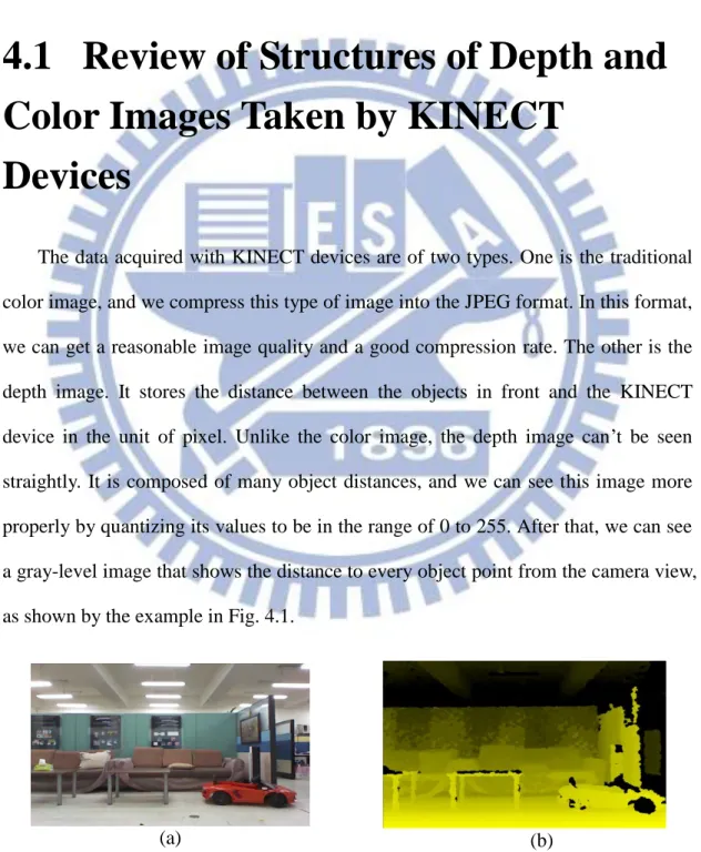
The data acquired with KINECT devices are of two types. One is the traditional color image, and we compress this type of image into the JPEG format. In this format, we can get a reasonable image quality and a good compression rate. The other is the depth image. It stores the distance between the objects in front and the KINECT device in the unit of pixel. Unlike the color image, the depth image can’t be seen straightly. It is composed of many object distances, and we can see this image more properly by quantizing its values to be in the range of 0 to 255. After that, we can see a gray-level image that shows the distance to every object point from the camera view, as shown by the example in Fig. 4.1.

(a) _(b)

30

4.2 Construction of 3D Images from

KINECT Images

4.2.1 Review of Pinhole Camera Model

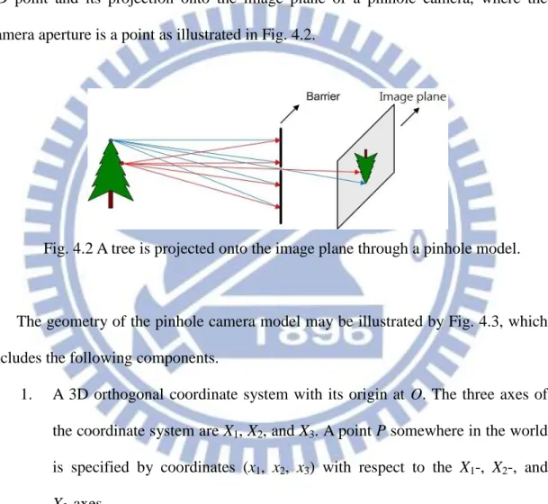
The pinhole camera model describes the relationship between the coordinates of a 3D point and its projection onto the image plane of a pinhole camera, where the camera aperture is a point as illustrated in Fig. 4.2.

Fig. 4.2 A tree is projected onto the image plane through a pinhole model.

The geometry of the pinhole camera model may be illustrated by Fig. 4.3, which includes the following components.

1. A 3D orthogonal coordinate system with its origin at O. The three axes of the coordinate system are X1, X2, and X3. A point P somewhere in the world

is specified by coordinates (x1, x2, x3) with respect to the X1-, X2-, and

X3-axes.

2. The image plane is parallel to the X1- and X2-axes. The image center is

denoted as R.

3. The projection of a space point P onto the image plane is denoted as Q. This point Q is just the intersection of the projection line (green) “emitted” by P and the image plane.

31

4. There is also a 2D coordinate system in the image plane, with its origin at R and its Y1- and Y2-axes parallel to the X1- and X2-axes, respectively. The

coordinates of point Q in this coordinate system are denoted as (y1, y2).

X2 X3 O X1 x1 x2 x3 Y1 Y2 P Q R Image plane f

Fig. 4.3 The geometry of a pinhole camera.

Next, we want to derive transformations between the coordinates (y1, y2) of point

Q and the coordinates (x1, x2, x3) of point P. In Fig. 4.4, we see two similar triangles

from which the following two equations can be derived:

3 1 1 x x f y _  ; (4.1) 3 2 2 x x f y   . (4.2)

Summarizing Equations 4.1 and 4.2, we get a vector equality as follows:

              2 1 3 2 1 x x x f y y . (4.3)

With the above equation, we can construct 3D images. The proposed method for this purpose will be explained in the next section.

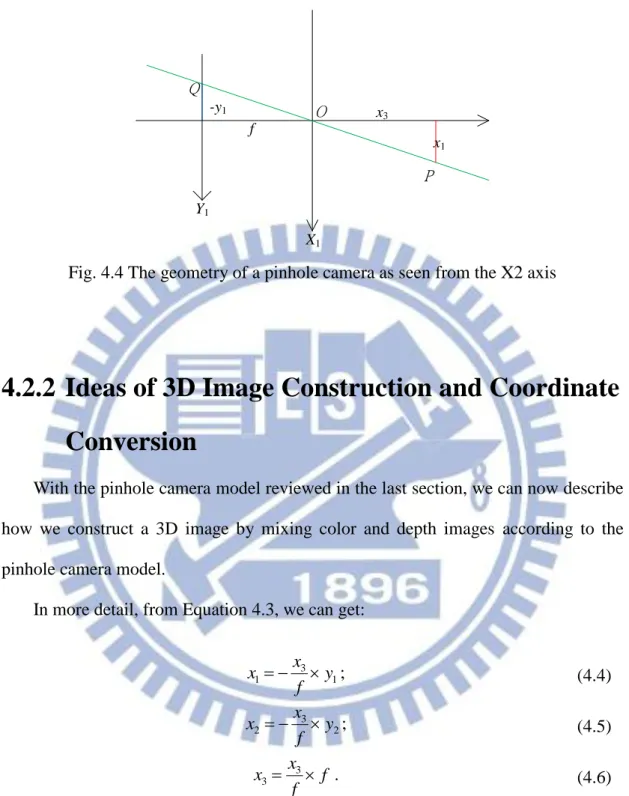
32 X1 O Y1 Q P x1 -y1 f x3

Fig. 4.4 The geometry of a pinhole camera as seen from the X2 axis

4.2.2 Ideas of 3D Image Construction and Coordinate

Conversion

With the pinhole camera model reviewed in the last section, we can now describe how we construct a 3D image by mixing color and depth images according to the pinhole camera model.

In more detail, from Equation 4.3, we can get:

And from Fig. 4.3, based on the similar-triangle principle again, we have the following equation: 1 3 1 y f x x   ; _(4.4) 2 3 2 y f x x   ; _(4.5) f f x x  3 3 . (4.6)

  



2 2 2 2 1 2 3 2 2 2 1 3 f y y x x x f x        (4.7)

33

where

  

2



2 2

1 2

y y f

    is the length of line segment OQ, and 2 2 2

1 2 3

x x x

is the length of line segment OP. In the same way, we can get:

For our applications here, from the above equations we can derive more detailed facts in the following which are useful for the purpose of 3D image construction:

1. 2 2 2

1 2 3

x x x is the distance between KINECT device and a point on the object, and we denote it as d;

2. the image center is R whose location is (Xmid,Ymid) in our captured depth

image by the KINECT device;

3. denote the focal length of the depth cameras by fd;

4. we can get Equations (4.10), (4.11), and (4.12) below from Equations (4.7), (4.8), and (4.9) for each point (xp, yp) in the depth image:

By (4.10), (4.11), and (4.12) , we can convert a 2D point with coordinates (xp, yp)

in a depth image into a 3D point with coordinates (x1, x2, x3) and construct the 3D

image by associating the corresponding color.

  



2 2 2 1 2 3 1 2 2 ₂ 1 1 2 x x x x y _{y y f}        ; (4.8)

  



2 2 2 1 2 3 2 2 2 ₂ 2 1 2 x x x x y _{y y f}        . (4.9)



 







1 _{2 2} 2 d p mi d p mi d p mi d d x x X x X y Y f        ; (4.10)



 







2 _{2 2} 2 d p mi d p mi d p mi d d x y Y x X y Y f        ; (4.11)



 



3 _{2 2} d 2 d p mi d p mi d d x f x X y Y f       . (4.12)

34

For the purpose of mapping 3D points to 2D pixels in the color image, we can derive, in a similar but inverse way, the following equations according to Equations (4.7), (4.8), and (4.9) (note that the focal length of the color camera is fC = 525):

where (Xmic, Ymic) are the image center of the color image.

Finally, we can construct a colorful 3D image from a depth image Id and a color

image Ic acquired by the KINECT device, and the details are described in the next

section.

4.2.3 Construction Algorithm and Experimental

Results

We have described each component of the proposed 3D image construction algorithm, and the full vision of this algorithm is presented below now.

Algorithm 4.1: construction of a 3D image.

Input: a color image Ic and a depth image Id acquired with a KINECT device. Output: a 3D image I3D constructed by the use of Ic and Id.

Steps:

Step 1. Transform the coordinates (xp, yp) and the depth value d of each pixel Pd in the

depth image Id into the 3D coordinates (x1, x2, x3) of Pd in the 3D space by

Equations (4.10), (4.11), and (4.12).

Step 2. Transform the 3D coordinates (x1, x2, x3) into 2D coordinates (xc, yc) in the

color image coordinate system by Equation (4.13) and (4.14).





c 1 3 c mi c f x X x x     => c 1 3 c mi c f x x X x     ; _(4.13)





c 2 3 c mi c f y Y x x     => c 2 3 c mi c f y x Y x     , _(4.14)

35

Step 3. Use (xc, yc) as indices to find the color values (R, G, B) of the pixel Pc at

coordinates (xc, yc) in the color image Ic.

Step 4. Take (R, G, B) as the color values of pixel Pd with coordinates (x1, x2, x3) in

the 3D space, and use these data (color values and 3D coordinates) to render a 3D color image I3D using the OpenGL as output.

The tool of OpenGL mentioned in Step 4 above can draw 3D points in the 3D space. It so can be used to draw the 3D image from different views so that we can see a constructed model or screen in the 3D image from a specific view by the projecting the points of the model or scene onto the chosen-view plane.

Depth images Color images Convert to 3D points Find corresponding color Realtime Recording Rendering 3D color points

Fig. 4.5 A flowchart of 3D image construction algorithm.

A result of applying Algorithm 4.1 is shown in Fig. 4.7, where the raw data (the original color image and depth image) are shown in Fig. 4.6. By Algorithm 4.1, the data can be converted into 3D format, and can be drawn with its corresponding color. Note that the black region represents no value of depth being available, so there is no

36

mapping to corresponding colors there.

(a) _(b)

Fig. 4.6 Images acquired by a KINECT device. (a) The depth image. (b) The color image.

(a)

(b)

Fig. 4.7 A constructed 3D image. (a) A perspective view of the 3D image. (b) A top view.

37

4.3 Review of a Method for Geometric

Correction of 3D Images

4.3.1 Idea of Geometric Correction

Once after we took a picture of a flat wall, which included both a depth image and a color one, and then conducted Algorithm 4.1, we found that the flat wall was a curved surface instead a plane when the resulting 3D image was displayed for inspection. The reason is that the infrared light rays emitted by the KINECT device are not all parallel to the X3-axis shown in Fig. 4.3, so that the we won’t get accurate

data.

A method has been proposed to solve this problem and is reviewed here. This curved surface was supposed to be of the shape of a paraboloid. Then, a paraboloid equation was derived for correcting this error. Specifically, after the paraboloid equation was found, the coordinates of x and y in the 3D image were substituted into this equation to get a corrected z value, as illustrated in Fig.4.8.

X Z O 2 2 p z    A x B y C C Error due to infrared light

38

4.3.2 Correction Algorithm and Experimental Results

Based on the above idea, an approximating paraboloid equation may be derived according to the criterion of minimum sum of squared errors (MSSE) in the following way.

(1) Let the equation of the paraboloid be written as:

where A and B are the quadratic coefficients and C is an intercepted length from the KINECT device to the apex of the paraboloid, as shown in Fig. 4.8.

(2) The equation for computing the value SSE of the SSE is:

where (xi, yi, zi) are the values of a 3D image pixel computed by

Algorithm 4.1 and h and w are the height and width of this depth image, respectively.

(3) To find the coefficients A, B and C, according to the minimum SSE criterion, the partial derivatives of Equation (4.16) with respect to variables

A, B and C, respectively are derived, yielding the following equations:

(4) The above simultaneous equations may be solved to obtain analytic solutions for the values of the coefficients A, B, and C.

2 2 p z  Ax By C. _(4.15)





2 2 2 0 i h w i i i i SSE z Ax By C      



_    _ . (4.16)



2 2

  

2 0 0 i h w i i i i i z Ax By C x           



; (4.17)



2 2

  

2 0 0 i h w i i i i i z Ax By C y           



; (4.18)



2 2



0 0 i h w i i i i z Ax By C          



. (4.19)

39

(5) The paraboloid is obtained by substituting A, B, and C back to (4.16).

Finally, we show two examples of the experimental results of applying the above scheme of geometric correction to 3D images in Figs. 4.9 and 4.10.

(a) (b)

Fig. 4.9 The 3D image of a wall seen from above. (a) Before correction. (b) After correction.

(a) (b)

Fig. 4.10 The 3D image of another wall seen from the top view. (a) Before correction. (b) After correction.

40

Chapter 5

Modeling of Around-car Objects

5.1 Introduction

In this chapter, we describe how we combine data acquired with multiple KINECT devices, and show the results in the same screen as a single view, like as a front view, a side view, or a rear view. Before this, we have to do calibration for the purpose of associating the parameters of the real world and those of the virtual world which is constructed in this study.

The calibration work in 3D space costs processing time, so we use a k-d tree to speed up our calibration steps. After this process, we know the relationship between each pair of neighboring KINECT devices. Then, we merge all the data to see a single view not only as a sparse point cloud, but also as a complete model which is constructed by many polygons. Since the 3D rendering bottleneck for model construction is the number of polygons, we try to reduce the number of polygons in our data without breaking its geometric property. The method of reduction is based on the use of the quadric error matrix (QEM). Before using the QEM, we have to construct polygons in the acquired depth images first. As a consequence, we can see a 3D image which is constructed by multiple KINECT data via real-time rendering. Moreover, the object in the screen which we want to tag such as cars or people is the

kinds of important information in a video surveillance. After that, we can add an index into each frame which includes the object information, so that the search of interesting objects or scenes can be made automatic without human involvement.

41

5.2 KINECT Camera Calibration

5.2.1 Review of Calibration of a Single KINECT

In this section, we will introduce how we get the focal length of the RGB-camera in the KINECT device, which we mentioned in the previous chapter and will be used in the calibration process. At first, we measure an object in the screen to know the object’s height py in the unit of pixel. Next, by the pinhole camera model again as

shown in Fig. 5.1, we can measure the distance dz from the object to the KINECT

device, as well as the object’s height h in the real world in the unit of mm. Then, we can apply the similar-triangle principle again to derive the following equation:

y

z

p h f d .

Finally, the focal length f can be obtained by solving the above equation to be

f = pydz/h. (5.1) O f Z Y py dz h

42

5.2.2 Transformation of Coordinates

In this section, we will introduce the method of coordinate transformation with6 degrees of freedom, which can be derived by two parts  one is translation, and the other is rotation.

First, we define a vector used in the transformation to be:

T = a b c           (5.2)

where a is the distance of translation in the X direction, b and c are interpreted similarly. Next, we define matrices for three ways of rotations, namely, pan, tilt, and swing, respectively, below:

RP= cos 0 sin 0 1 0 sin 0 cos P P P P               ; (5.3) RT= 1 0 0 0 cos sin 0 sin cos T T T T        _        ; (5.4) RS= cos sin 0 sin cos 0 0 0 1 S S S S                , (5.5)

where P is the pan angle, T is the tilt angle, and S is the swing angle. Then, a total

43 R= cos sin 0 sin cos 0 0 0 1 S S S S                1 0 0 0 cos sin 0 sin cos T T T T        _        cos 0 sin 0 1 0 sin 0 cos P P P P               , (5.6) or equivalently, to R=

cos cos sin sin sin sin cos cos sin sin sin cos

sin cos cos sin sin cos cos sin sin cos sin cos

cos sin sin cos cos

S P S T P S T S P S T P S P S T P S T S P S T P T P P T P                                    _{ }         .

As a result, if a point P1 become P1' after the transformation, we can express P1'

as

P1' = RP1 + T (5.7)

for some P, T, S, a, b, and c. This concludes our review of the coordinate

transformation process, and this process will be used in the next section for our application of 3D scene modeling.

5.2.3 Review of Iterative Closest Point (ICP)

Algorithm

The ICP algorithm is a method useful for 3D model alignment [6-8]. In this section, we will introduce the operation of the ICP step by step, and describe the bottleneck of the algorithm.

First, the original ICP algorithm is basically a brute-force method for aligning two clusters of points which are used to construct a scene or object model. The core idea of this algorithm is that “each point in one group finds a closest point in the other group.” More points this rule is satisfied by, more possibly the corresponding transformation (including the translation and rotation) is true. The detail of this

44

algorithm is shown below.

Algorithm 5.1: aligning two groups of points in a 3D space. Input: Two groups of points, Pa and Pb.

Output: A translation matrix T and a rotation matrix R for aligning Pa and Pb. Steps:

Step 5. Make a little change of T and R on Pb, and compute Pb' = PbR + T. where R

and T are as described in Section 5.2.2 (leading to Equation 5.7).

Step 6. For each point b in Pb', find the closest point s to it in Pa, and calculate the

Euclidean distance dbs between b and s.

Step 7. After all the points in Pb' have been processed, sum up all the distances to get

 

b min bs b P D d  



Step 8. If Dmin is the minimal in all the possible changes of transformation and

rotation, then the corresponding T and R are the transformation and rotation matrices for aligning the two groups of points, Pa and Pb.

From the algorithm described above, we know that the speed bottleneck is Step 2 since for each point in one group, we have to check all the points in the other group by brute force. An improved method is proposed in the next section.

5.2.4 Calibration by the ICP algorithm Using

Speeded-up k-d Tree

In this section we introduce how k-d tree can be utilized to speed up Algorithm 5.1. First, it is noted that the k-d tree is a data structure for “partitioning the 3D space.” After such partitioning, we can speed up Algorithm 5.1. In Step 2 of