室內環境之三維模型重建

(1)

國

立

交

通

大

學

資訊科學與工程研究所

碩

士

論

文

室內環境之三維模型重建

Three-Dimensional Surface Model

Reconstruction of Indoor Environments

研究生：張凱為

指導教授：陳永昇教授

(2)

室內環境之三維模型重建

Three-Dimensional Surface Model

Reconstruction of Indoor Environments

研究生：張凱為 Student：Kai-Wei Chang

指導教授：陳永昇 Advisor：Yong-Sheng Chen

國立交通大學

資訊科學與工程研究所

碩士論文

A Thesis

Submitted to Institute of Computer Science and Engineering College of Computer Science

National Chiao Tung University in partial Fulfillment of the Requirements

for the Degree of Master

in

Computer Science

June 2007

Hsinchu, Taiwan, Republic of China

(3)

摘要

從二維的影像資訊重建出三維的場景模型，一直是電腦視覺領域一個重要的研究主題，隨著電腦計算速度的進步，這項研究所延伸而出的應用更是琳瑯滿目。近年來蓬勃發展的電腦繪圖、虛擬實境等等，都會利用到影像重建的技術，比如將一些現成的玩具利用多個視角的照片，便可在電腦中產生玩具的模型。我們提出了一個透過影像來重建三維場景模型的方法，透過影像之中與影像之間的關係將攝影機的內外部參數算出之後，我們變能夠將影像間重複拍攝的部份的三維座標點算出。在算出三維座標點之後，使用Wendland將三維座標點之間缺乏的部份算出來形成場景的三維表面模型並將拍攝到的影像當作場景的材質貼到該模型上以達到擬真的室內環境重建。

(4)

致謝

本篇論文的完成，首先要感謝我的指導教授陳永昇老師，在老師熱心的協助之下，不論是在學術的研究上，或是在論文撰寫的過程中，都給了我莫大的幫助，也使得本篇論文能夠順利地完成。也謝謝口試委員莊仁輝教授及黃仲陵教授給予我的建議與指教，使得本篇論文能夠更加完善。另外，也感謝實驗室的同學和學長姊學弟妹，因為有他們的相互扶持與陪伴，使我的研究過程並不孤單。最後，我要謝謝我的家人，因為他們的支持是我努力的最大動力，僅以此篇論文，獻給我最愛的父母親。

(5)

Three-Dimensional Surface Model

Reconstruction of Indoor Environments

A thesis presented

by

Kai-Wei Chang

to

Department of Computer Science

and Information Engineering

in partial fulfillment of the requirements for the degree of

Master of Science

in the subject of

Computer Science and Information Engineering

National Chiao Tung University Hsinchu, Taiwan

(6)

Three-Dimensional Surface Model Reconstruction of Indoor Environments

Copyright c₂₀₀₇ by

(7)

Abstract

In recent years computer hardware and computer graphics has made tremendous progress in visualizing 3D models of real objects. Many techniques have reached maturity and are being ported to hardware. This seems like in the area of 3D visualization, performance may increase even faster than Moor’s law. Some job required a million dollar computer a few years ago can be now achieved by a custom computer, which cost a few hundred dollars. It is now possible to visualize complex 3D scenes in real time due to the advancement of computer hardware.

This speed of evolution causes an essential demand for more complex and realistic models. Even though we are now able to build three-dimensional models, the tools for three-dimensional modeling are getting more and more powerful, synthesizing realistic models is difficult and time-consuming. Many virtual objects are inspired by real objects, so we are interested in being able to build three-dimensional environment models directly from the real environments.

In the past, visual inspection and robot guidance were the main applications. We re-quire more and more 3D content for computer graphics, virtual reality and communication nowadays. The visual quality becomes one of the main points of attention. Therefore not only the position of a small number of points have to be measured with high accuracy, but the geometry and appearance of all points of the surface have to be measured.

We proposed a semi-automatic 3D indoor environment reconstruction procedure using the thin-plate splines for surface modeling and texture mapping. First, the intrinsic parame-ters of the two cameras are calibrated. Second, calculate the fundamental matrix by using the well-known Eight-Point algorithm and the essential matrix is derived to be the combi-nation of fundamental matrix and the two camera intrinsic matrices. Third, relative pose of the two cameras can be extracted from the essential matrix and sparse 3D point recon-struction can be performed. Forth, interpolate 3D surfaces among the reconstructed sparse 3D points with the thin-plate splines. Finally, we can add textures on the reconstructed 3D surface model with some texture mapping techniques. The 3D surface model established

(8)

with the proposed reconstruction system provides useful information for robot navigation and other applications.

(9)

Acknowledgements

(10)

(11)

List of Figures

1.1 A 3D Laser Scanner . . . 2

1.2 3D Laser Scanning Result - Human Face . . . 3

1.3 3D Laser Scanning Result - Shoe . . . 4

1.4 An image of a scene with some features specified. . . 5

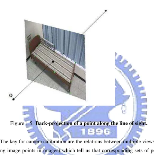
1.5 Back-projection of a point along the line of sight. . . 6

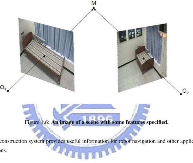
1.6 An image of a scene with some features specified. . . 7

2.1 Camera 3D Reconstruction System - 3D Dome Developed by Narayanan, Rander and Kanade. . . 10

3.1 Shapes which are equivalent to a cube under different geometric transforms. 25 4.1 Perspective Camera Model. . . 29

4.2 From Image Coordinates to Retinal Coordinates. . . 30

4.3 Correspondences Between Two Views. . . 32

4.4 Two-View Epipolar Geometry. . . 33

4.5 The Pose Recovery Twisted Pair Extracted from The Essential Matrix. . . . 39

5.1 Radio Basis Function of the Thin-Plate Splines in Two-Dimensional Space. 44 5.2 A Mathematical Model of A Thin Steel Plate. . . 45

6.1 Our 2D Planar Camera Calibration Planar Pattern. . . 57

6.2 Result Image After Binarization. . . 57

6.3 Result Image After Grid Alignment. . . 58

6.4 Multi-view Photos For 3D Environment Reconstruction With Correspond-ing Image Points Specified - Scene 1. . . 58

(14)

6.5 Multi-view Photos For 3D Environment Reconstruction With

Correspond-ing Image Points Specified - Scene 2. . . 59

6.6 Multi-view Photos For 3D Environment Reconstruction With Correspond-ing Image Points Specified - Scene 3. . . 59

6.7 Scene 1 - Epipolar Lines Calculated With The Fundamental Matrix. . . 61

6.8 Scene 2 - Epipolar Lines Calculated With The Fundamental Matrix. . . 61

6.9 Scene 1 Viewpoint 1 - Individually Reconstructed Surface Model. . . 62

6.20 Viewpoint 1 - Reconstructed Environment Using Our Method. . . 68

6.26 Wireframe - Projecting all the synthesized views onto a sphere. . . 71

6.27 Wireframe - Reconstructed part of all the synthesized views. . . 71

6.28 Textured model - Projecting all the synthesized views onto a sphere. . . 72

6.29 Textured model - Reconstructed part of all the synthesized views. . . 72

(15)

List of Tables

3.1 Comparison of Different Geometric Strata . . . 24 6.1 The Specification of Our 3D Environment Recontruction System. . . 51 6.2 The Calibrated Pan-Tilt-Zoom Camera Intrinsic Parameters Using Our

Cal-ibration Method. . . 60

(16)

(17)

Chapter 1 Introduction

(18)

2 Introduction

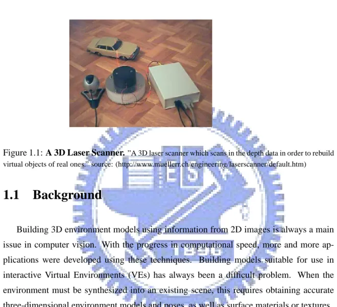
Figure 1.1: A 3D Laser Scanner.”A 3D laser scanner which scans in the depth data in order to rebuild virtual objects of real ones.” source: (http://www.muellerr.ch/engineering/laserscanner/default.htm)

1.1 Background

Building 3D environment models using information from 2D images is always a main issue in computer vision. With the progress in computational speed, more and more ap-plications were developed using these techniques. Building models suitable for use in interactive Virtual Environments (VEs) has always been a difficult problem. When the environment must be synthesized into an existing scene, this requires obtaining accurate three-dimensional environment models and poses, as well as surface materials or textures.

In addition to the appearance of the reconstructed environment, modeling the behav-iour of objects is also very important if the system and the environment allow any kind of nonpassive user interaction. Generally, a scene hierarchy is constructed by specifying the relationships between objects in the scene. These relationships can then be used to assist the user in interacting with the environment.

Traditional methods of reconstructing environment models involve a skilled user and a three-dimensional CAD (Computer Aided Design) program. Accurately modeling a real environment in such a way can only be done if the user has obtained blueprints is able

(19)

1.1 Background 3

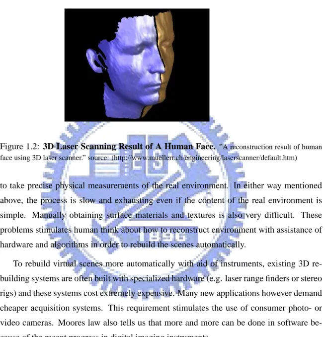
Figure 1.2: 3D Laser Scanning Result of A Human Face. ”A reconstruction result of human face using 3D laser scanner.” source: (http://www.muellerr.ch/engineering/laserscanner/default.htm)

to take precise physical measurements of the real environment. In either way mentioned above, the process is slow and exhausting even if the content of the real environment is simple. Manually obtaining surface materials and textures is also very difficult. These problems stimulates human think about how to reconstruct environment with assistance of hardware and algorithms in order to rebuild the scenes automatically.

To rebuild virtual scenes more automatically with aid of instruments, existing 3D re-building systems are often built with specialized hardware (e.g. laser range finders or stereo rigs) and these systems cost extremely expensive. Many new applications however demand cheaper acquisition systems. This requirement stimulates the use of consumer photo- or video cameras. Moores law also tells us that more and more can be done in software be-cause of the recent progress in digital imaging instruments.

Due to the factors mentioned above, many techniques using informations captured from cameras have been developed over the last few years. Many of these techniques do not require more than some cameras and a computer to rebuild three-dimensional models of real objects.

(20)

how-4 Introduction

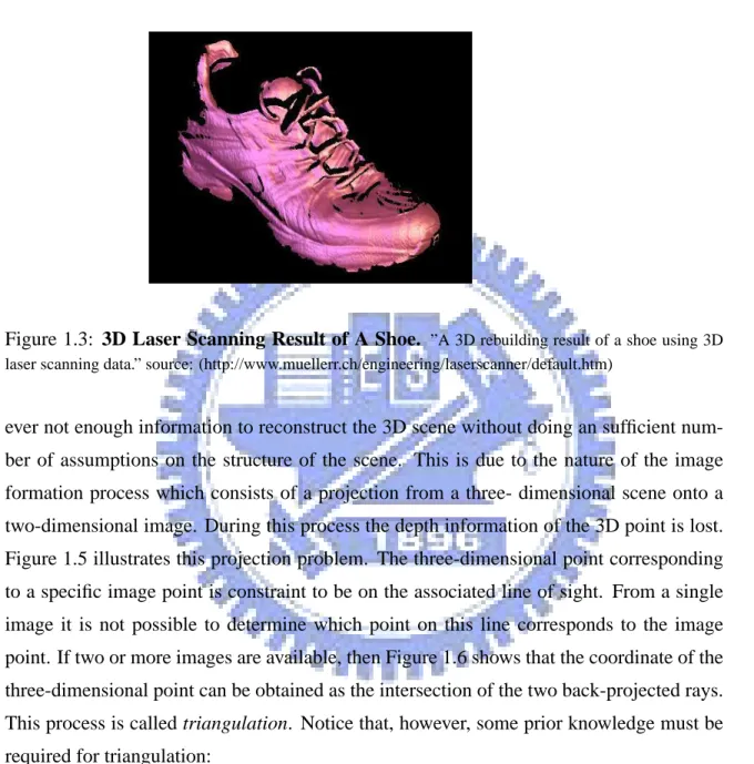
Figure 1.3: 3D Laser Scanning Result of A Shoe. ”A 3D rebuilding result of a shoe using 3D laser scanning data.” source: (http://www.muellerr.ch/engineering/laserscanner/default.htm)

ever not enough information to reconstruct the 3D scene without doing an sufficient num-ber of assumptions on the structure of the scene. This is due to the nature of the image formation process which consists of a projection from a three- dimensional scene onto a two-dimensional image. During this process the depth information of the 3D point is lost. Figure 1.5 illustrates this projection problem. The three-dimensional point corresponding to a specific image point is constraint to be on the associated line of sight. From a single image it is not possible to determine which point on this line corresponds to the image point. If two or more images are available, then Figure 1.6 shows that the coordinate of the three-dimensional point can be obtained as the intersection of the two back-projected rays. This process is called triangulation. Notice that, however, some prior knowledge must be required for triangulation:

• Corresponding image points

• Relative pose of the camera for the different views

(21)

1.2 Thesis Scope 5

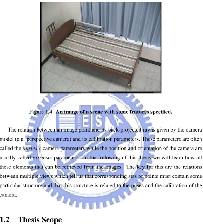
Figure 1.4: An image of a scene with some features specified.

The relation between an image point and its back-projected ray is given by the camera model (e.g. perspective camera) and its calibration parameters. These parameters are often called the intrinsic camera parameters while the position and orientation of the camera are usually called extrinsic parameters. In the following of this thesis we will learn how all these elements that can be retrieved from the images. The key for this are the relations between multiple views which tell us that corresponding sets of points must contain some particular structure and that this structure is related to the poses and the calibration of the camera.

1.2 Thesis Scope

In this thesis, we proposed a 3D reconstruction procedure using images captured by cameras at different poses. The relation between an image point and its corresponding ray of sight is given by the camera model (e.g. perspective camera) and the camera calibration parameters. These parameters are often called the intrinsic camera parameters while the position and orientation of the camera are in general called camera extrinsic parameters. In the following chapters we will learn how all these elements can be acquired from the

(22)

6 Introduction

Figure 1.5: Back-projection of a point along the line of sight.

images. The key for camera calibration are the relations between multiple views (e.g. cor-responding image points in images) which tell us that corcor-responding sets of points must contain some structure and that this structure is related to the intrinsic and extrinsic para-meters of the camera.

In our 3D reconstruction procedure, first, the intrinsic parameters of the two cameras are calibrated. Second, we calculate the fundamental matrix by using the well-known Eight-Point algorithm and the essential matrix is derived to be the combination of fundamental matrix and the two camera intrinsic matrices. Third, relative pose of the two cameras can be extracted from the essential matrix and sparse 3D point reconstruction can be performed. Fourth, interpolate 3D surfaces among the reconstructed sparse 3D points with the thin-plate splines. Finally, we can add textures on the reconstructed 3D surface model with some texture mapping techniques. The 3D surface model established with the proposed

(23)

1.3 Thesis Organization 7

Figure 1.6: An image of a scene with some features specified.

reconstruction system provides useful information for robot navigation and other applica-tions.

1.3 Thesis Organization

After this chapter, we will introduce some relative works during the pass few years. Chapter 3 describes projective geometry and the stratification of geometric structure. After some geometric fundamentals are introduced, we turn into the perspective camera model and some geometric calculation of the relation between multiple view cameras in chapter 4. Chapter 5 tells the main 3D surface modeling method we use to reconstruct photo texture

(24)

8 Introduction

mapped 3D models in this thesis and then run the way through to perform our 3D model reconstruction procedure in chapter 6. Some reconstruction and experiment results are shown in chapter 7 and finally, we have some conclusion and future works discussed in chapter 8.

(25)

Chapter 2

(26)

10 Related Works

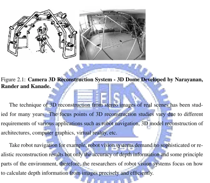
Figure 2.1: Camera 3D Reconstruction System - 3D Dome Developed by Narayanan,

Rander and Kanade.

The technique of 3D reconstruction from stereo images of real scenes has been stud-ied for many years. The focus points of 3D reconstruction studies vary due to different requirements of various applications such as robot navigation, 3D model reconstruction of architectures, computer graphics, virtual reality, etc.

Take robot navigation for example, robot vision systems demand no sophisticated or re-alistic reconstruction results but only the accuracy of depth information and some principle parts of the environment, therefore, the researchers of robot vision systems focus on how to calculate depth information from images precisely and efficiently.

Another example is the 3D virtual model reconstruction of a specific real object, the most common way nowadays is to put the object on a rotating plate and keep capturing images with a stationary camera while the plate rotates. The camera can be calibrated first in order to acquire the relationship between image points and its reprojection rays. Camera motion can be formulated since the rotation speed and the radius of the rotation are prior knowledge under the model reconstruction system. The main purpose of 3D virtual model reconstruction systems is to build photo-realistic models from a sequence of images.

In the following sections of this chapter, we will introduce several methods about how to rebuild 3D virtual models from images captured by various poses of cameras.

(27)

2.1 Multi-View 3D Reconstruction 11

2.1 Multi-View 3D Reconstruction

Multi-view 3D reconstruction systems rebuild the model from photos captured by sev-eral cameras of different poses. The corresponding features are found amoung cameras in order to calculate 3D coordinates of the real object. Cameras in multi-view rebuilding sys-tems are often fully calibrated so that their relative poses are known. Acquire enough 3D information by tracking the motion of an moving object with multiple calibrated cameras is the main advantage of these systems.

Narayanan, Rander and Kanade proposed a multi-view photographic reconstruction system called 3D Dome [12]. As illustrated in Figure 2.1, the system 3D Dome is a semi-sphere multi-capturing system formed by fifty-one synchronous and fully calibrated cam-eras. Since all the cameras are all fully calibrated, which means in the Equation 4.6 the camera intrinsic matrix K and relative poses amoung cameras are all known. Therefore, when a person is taking some actions in the 3D dome, every camera around the 3D dome will capture images from different point of views and then obtain a dense depth graph for each camera by running through a multiple-baseline stereo reconstruction procedure. Map-ping the texture onto the dense depth graph forms a simple reconstructed 3D human model. The author called this a visible surface model (VSM). But VSM is a surface model recon-structed from each camera, there is some part of the human have inevitable reconstruction difficulties due to occlusion. The author solved this problem by synthesizing all the VSMs together with a optimized integration procedure in order to reconstruct the complete surface

model (CSM) of the scene.

In the 3D dome system, cameras are all fully calibrated with relative poses known. Therefore, in the 3D dome system, calculation of 3D coordinates from the photos needs no complicated computation. Since the system is equipped with 51 cameras, the main problem of the system is to have cameras capture images synchronously.

Fua and Leclerc have proposed a similar system which goal is to rebuild the real scenes in virtual reality [6]. Differ from Narayanan, Rander and Kanade, they use only two cali-brated cameras to capture images of static scenes. Fua and Leclerc turn the calculated 3D points into meshes in order to reconstruct the 3D surface model of the scenes.

(28)

12 Related Works

2.2 Single-Camera 3D Reconstruction

Single-camera 3D reconstruction systems often obtain images with a single camera but from different point of view or simply record videos while the camera is moving. The most often used method is the so-called structure from motion. Image processing methods, such as multi-image intensity correlation, can be used in single camera video systems in order to find out image correspondences since there should be small differences between frames in short-term intervals.

Pollefeys and Van Gool [13] have implemented a single camera reconstruction system similar to described systems above. The input of their system is a sequence of images captured from the same scene by single camera. After specifying some distinct features in each image, similarity comparison methods are used to find out correspondences amoung images. Since there are some errors in images due to camera projection hardware structure and some noises caused if the feature points were specified by human, Pollefeys and Van used a method called random sampling consesus(RANSAC) to calculate several choices of the fundamental matrices from the image correspondences and picked the most stable fundamental matrix out from the computed matrices. The fundamental matrix encodes the transformation of every image points in two corresponding images, the definition of the fundamental matrix and epipolar geometry will be introduced in chapter 3 and 4. After finding out the fundamental matrix, a projective reconstruction can be computed. If the cameras are calibrated, the intrinsic parameters of the camera matrix are all known and thus a metric reconstruction can be performed, which differs from the real world by only a scalar factor. After the metric reconstruction is done, the author computed the dense depth graph in order to calculate depth for every pixel in the image and then performed texture mapping to reconstruct the whole 3D model.

Fitzgibbon and Zisserman have proposed a similar system, but besides finding feature points, they used the informations of line segments in the images by using image processing techniques such as edge detection for 3D reconstruction. Therefore, their reconstruction re-sults are not only sparse 3D points but with the information support of line segments, which can assist in reducing the depth error of the 3D reconstruction. In addition, Zisserman used

(29)

2.3 Other Reconstruction Methods and Applications 13

both the two-view reconstruction method and the trifocal tensor method, which is to cut down depth ambiguity by using three-view image correspondences.

2.3 Other Reconstruction Methods and Applications

There are lots of applications require image-based 3D reconstruction systems for assis-tance. Schreer [15] has developed a robot navigation system with photographic 3D recon-struction algorithms built in. The two cameras used for robot vision are both fully calibrated in order to calculate 3D coordinates in real-time while the robot is moving around in the environment. But this system uses only the distribution condition of the reconstructed 3D points with some prior knowledge and experiences in order to avoid obstacles. But lack of considering the structure of indoor environments may cause the robot vision system inflexible.

Some reconstruction systems use some characteristics of the scenes to refine the recon-structed model. Cipolla and Robertson [3] used the prior knowledge such as the perpen-dicular relations amoung walls and floors of the buildings to find the vanishing point in the image. The vanishing point is then transfered into a 3D vector form in order to reduce computational error of the vanishing point. After the vanishing point is found, the cam-era intrinsic parameters can be calculated with the vanishing point in order to simplify the calculation process of camera intrinsic parameters and 3D model reconstruction.

(30)

(31)

Chapter 3

(32)

16 Projective geometry

The concepts presented in the following two chapters concentrates on concepts of pro-jective geometry. This chapter and the next one introduce most of the geometric concepts used in the rest of the thesis. This chapter focuses on projective geometry and introduces concepts as points, lines an planes in two or three dimensions. A lot of attention goes to the analysis of geometry in projective, affine, metric and Euclidean layers. Projective geome-try is used for its simplicity in formalism, additional structure and properties that can then be introduced were needed through this hierarchy of geometric strata. This section was in-spired by the introductions on projective geometry found in Faugeras’ book [5]. A detailed description on the subject can be found in the recent book by Hartley and Zisserman [8].

3.1 Projective Geometry

A point in projective n-space _Pn is given by a (n + 1)-vector of coordinates x = [x1...xn+1]T. At least one of these entries of the vector should differ from zero. These

coordinates are called homogeneous coordinates. In this thesis the coordinate vector and the point itself will be denoted with the same symbol. Two points denoted by (n +

1)-vectors x and y are equal if and only if there exists a nonzero scalar λ such that x = λy.

This will be indicated by x_{∼ y.}

A collineation is a mapping between projective spaces. A collineation from _Pm _to

Pn _{can be mathematically denoted by a}

(m + 1) × (n + 1) matrix H, where points are

transformed linearly: x0 _{∼ Hx. Matrices H and λH with a nonzero scalar λ represent the} same collineation.

A projective basis is the extension of a coordinate system to projective geometry. A projective basis is a set of n+ 2 points such that no n + 1 of them are linearly dependent.

The set el = [0, · · · , 1, · · · , 0]T, ∀l, 1≤l≤n + 1, where 1 is in the lth position and en+2 =

[1, 1, · · · , 1]T _{is the standard projective basis. A projective point of}

Pn_{can be described as}

a linear combination of any n+ 1 points of the standard basis. For example: m =

n+1

X

l=1

(33)

3.1 Projective Geometry 17

It can be shown [4] that any projective basis can be transformed into a unique collineation of the standard projective basis. Similarly, if two sets of points m1, ..., mn+2and m01, ..., m0n+2

both form a projective basis, then there exists a uniquely resolved collineation T such that

ml0 ∼ T ml, ∀l, 1≤l≤n + 2. This collineation T describes the different combination of

projective basis. Notice that T is invertible.

3.1.1 The Projective Plane

The projective plane is the projective space _P2. A point in_P2 is represented by a 3-vector m= [x, y, z]T_{. A line l is also represented by a 3-vector. A point m is located on a}

line l if and only if

lTm= 0 (3.1)

This equation, however, can also be described as the expression that ”the line l passes through the point m” or ”the point m in on the line l”. This symmetry in the equation shows that there is no formal difference between points and lines in the projective plane. This is known as the principle of duality. A line l passing through two points m1 and m2 is given

by their vector product m1 × m2. This can also be written as

l_{∼ [m}1]xm2, with[m1]x=       0 z1 −y1 −z1 0 x1 y1 −x1 0       (3.2)

The dual formulation gives the intersection of two lines. All the lines passing through a specific point form a pencil of lines. If two lines l1 and l2 are distinct elements of the

pencil, all the other lines can be obtained through the following equation:

l_{∼ λ}1l1+ λ2l2 (3.3)

(34)

3.1.2 The Projective 3D Space

A projective 3D space typically means the dimension of the projective space is 3, where is the projective space _P3. An element in _P3 is represented by a 4-entry vector M = [X, Y, Z, W ]T_{. In}

P3 _{the duality of an element is a plane, which is also denoted as a}

4-entry vector. A point M lies on a planeΠ can be denoted mathematically as:

ΠT_M _{= 0}

(3.4) A line can be written into a linear combination of two points as:

λ1M1+ λ2M2

or can be produced by the intersection of two planesΠ1 ∩ Π2.

3.1.3 Projective Transformations

We can denote a transformation between the images as a homography of _P2 _{→ P}2 , which can be represented by a_{3 × 3-matrix H. With the same properties of matrices, H} and λH represent the same homography for all nonzero scalars λ. A point is transformed as follows:

m_{7→ m}0 _{∼ Hm} (3.5)

The corresponding transformation of a line can be obtained by transforming the points which are on the line and then finding the line defined by these points:

l0Tm0 = lTH−1Hm= lTm= 0 (3.6) From the previous equation it is easy to derive a transformation equation for a line (H−T = (H−1₎T _{= (H}T₎−1_):

(35)

3.2 Analysis of 3D Geometry 19

Similar reasons can be considered in_P3 gives the following equations for transforma-tions of points and planes in 3D space:

M _{7→ M}0 _{∼ T M,} (3.8)

Π 7→ Π0 ∼ T−TΠ (3.9) where T is a_{4 × 4-matrix.}

3.2 Analysis of 3D Geometry

Usually we define the real world as a Euclidean 3D space. But in some particular cases it is not sufficient to use the full Euclidean structure of 3D space. Euclidean 3D space is only suitable for less structured and thus simpler projective geometry. Intermediate layers are formed by the affine and metric geometry. These structures can be thought of as different geometric layers which can be overlaid on the world for different transformations. The most complicated is Euclidean, then metric, next affine and finally projective structure. The concept of stratification is closely related to the groups of transformations acting on geometric entities and leaving some properties of configurations of these elements in-variant. Attached to the projective stratum is the set of projective transformations, attached to the affine stratum is the set of affine transformations, attached to the metric stratum is the set of similarities and attached to the Euclidean stratum is the set of Euclidean transforma-tions. It is important to notice that these groups are subgroups of each other, e.g. the metric group is a subgroup of the affine group and both are subgroups of the projective group.

An important aspect related to these groups are their invariants. An invariant is a prop-erty of a derivation of geometric entities that is not altered by any transformation belonging to a specific group. Invariants therefore can guild us what measurements we can do consid-ering a specific stratum of geometry. These invariants are often related to geometric entities which stay unchanged after applying the transformations to a specific group. These

(36)

geomet-20 Projective geometry

ric entities with invariants related play an important role in part of this thesis.Recovering them allows us to upgrade the structure of the geometry to a higher level of the geometric stratification.

In the following sections, different strata of geometry are discussed. The associated groups of transformations, their invariants and the corresponding invariant structures are presented.

3.2.1 Projective Stratum

The simplest stratum is the projective stratum. It is the less structured one and has the least number of invariants and the largest group of transformations related to it. The group of projective transformations or collineations is composed with the most general group of linear transformations.

A projective transformation of 3D space can be denoted by a _{4 × 4-matrix, where the} matrix is invertible: TP ∼          p11 p12 p13 p14 p21 p22 p23 p24 p31 p32 p33 p34 p41 p42 p43 p44          (3.10)

This transformation matrix is only defined up to a nonzero scale factor and has therefore 15 degrees of freedom.

Relations of collinearity, incidence and tangency are projectively invariant. The cross-ratio is an invariant property under projective transformations as well. It is defined as follows: Assume that the four points M1, M2, M3 and M4 are collinear. Then they can be

expressed as Mi = M + λiM0 (assume none is coincident with M0). The cross-ratio is

defined as {M1, M2; M3, M4} = λ1− λ3 λ1− λ4 :λ2− λ3 λ2− λ4 (3.11)

(37)

The cross-ratio does not depend on the choice of the reference points M and M0 and is invariant under the group of projective transformations of _P3. It can be derived that a similar cross-ratio invariant for four line intersecting in a point or four planes intersecting in a line.

We can regard cross-ratio as the coordinate of the fourth point is the linear combination of the first three points, since three points form a basis for a projective line in_P1. Similarly, two invariants can be found for five coplanar points, three invariants for six coplanar points, all in general position.

3.2.2 Affine Stratum

The affine stratum has more structure than the projective one, but less structure than the metric or the Euclidean strata. Differs from projective stratum, the affine stratum identifies a special plane, which called the plane at infinity.

To define this plane at infinity, we have W = 0 and thus Π∞ = [0, 0, 0, 1]T. We can

consider that the projective space contains the affine space under the one-to-one mapping:

A3 _{→ P}3_{: [X, Y, Z]}T _{7→ [X, Y, Z, 1]}T_{. The plane W} _{= 0 in P}3 _{can be thought as}

con-taining the limit points for_{kMk = ∞. The Affine transformation is usually denoted as the} following:       X0 Y0 Z0       =       a11 a12 a13 a21 a22 a23 a31 a32 a33             X Y Z       +       a14 a24 a34       , with det(aij)6= 0 (3.12)

The affine transformation can be rewritten in the matrix form: M0 _{∼ T}AM with:

TA∼          a11 a12 a13 a14 a21 a22 a23 a24 a31 a32 a33 a34 0 0 0 1          (3.13)

(38)

Therefore, the affine transformation has 12 independent degrees of freedom. All in-variants under the projective stratum also exsist under the affine stratum. For the more restrictive affine group, parallelism is added as a new invariant property. Lines or planes having their intersection at infinity are called parallel. Another new invariant property for affine group is the ratio of lengths along some direction.

3.2.3 Metric Stratum

The metric stratum resembles in the group of similarities. This stratum differs from the Euclidean stratum only up to a scale factor. The metric transformations correspond to Euclidean transformations complemented with a scaling. When no absolute measure-ment is available, reconstruction in the metric coordinate is the highest level of geometric structure that 3D reconstruction from images can achieve.

A metric tranformation can be represented as the following:

      X0 Y0 Z0       = σ       r11 r12 r13 r21 r22 r23 r31 r32 r33             X Y Z       +       t14 t24 t34       (3.14)

with rij the coefficients of an orthonormal matrix, which is usually denoted by R such

that RTR= RRT _{= I and thus R}−1 _{= R}T_{. Recall that R is a rotation matrix if and only if}

RRT _{= I and det(R) = 1. In homogeneous coordinates, Equation 3.14 can be rewritten as}

M0 = TMM , with TM ∼          σr11 σr12 σr13 tX σr21 σr22 σr23 tY σr31 σr32 σr33 tZ 0 0 0 1          ∼          r11 r12 r13 σ−1tX r21 r22 r23 σ−1tY r31 r32 r33 σ−1tZ 0 0 0 σ−1          (3.15)

A metric transformation therefore has 7 independent degrees of freedom, 3 for trans-lation, 3 for orientation and 1 for scale. In metric stratum there are two important new invariants properties: relative lengths and angles.

(39)

3.2.4 Euclidean Stratum

The only difference between Euclidean stratum and metric stratum is absolute length. Therefore, the Euclidean transformation has 6 independent degrees of freedom, 3 for trans-lation and 3 for rotation. A Euclidean transformation has the following matrix form:

TE ∼          r11 r12 r13 tX r21 r22 r23 tY r31 r32 r33 tZ 0 0 0 1          (3.16)

with rij the coefficients of an orthonormal matrix, as described previously. If det(R) =

1 then, this transformation is simply the same as a rigid-body transformation in space.

3.2.5 Comparison of the Different Strata

In this chapter some concepts of projective geometry were introduced. Based on these concepts, some methods can be invented by doing the inverse of the projection process and obtain 3D reconstructions of the observed scenes, where is the main objective of this thesis. We can list a table in order to compare different strata described previously:

(40)

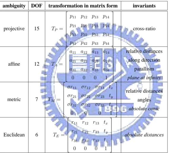
ambiguity DOF transformation in matrix form invariants

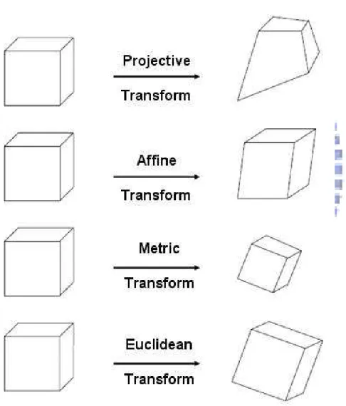
projective 15 TP =          p11 p12 p13 p14 p21 p22 p23 p24 p31 p32 p33 p34 p41 p42 p43 p44          cross-ratio affine 12 TA=          a11 a12 a13 a14 a21 a22 a23 a24 a31 a32 a33 a34 0 0 0 1          relative distances along direction parallism plane at infinity metric 7 TM =          σr11 σr12 σr13 tx σr21 σr22 σr23 ty σr31 σr32 σr33 tz 0 0 0 1          relative distances angles absolute conic Euclidean 6 TE =          r11 r12 r13 tx r21 r22 r23 ty r31 r32 r33 tz 0 0 0 1          absolute distances

Table 3.1: Comparison of Different Geometric Strata. ”Number of degrees of freedom, trans-formation in matrix form and invariants corresponding to different geometric strata.”

(41)

Figure 3.1: Shapes which are equivalent to a cube under different geometric transforms.

(42)

(43)

Chapter 4 Camera Model and 3D Reconstruction

Fundamentals

(44)

28 Camera Model and 3D Reconstruction Fundamentals

Before discussing how to reconstruct 3D objects from relations of images captured from different poses of cameras, it is important to know how images are formed via the camera model. In the following sections, first, the perspective camera model is introduced. Second, some important relationships between multiple views are presented with some mathematics.

4.1 The Camera Model

In this thesis the model of perspective camera is used. The image-forming process is completely determined by having a perspective projection center point and a retinal plane. The projection of a real 3D point is then obtained as the intersection of a line passing through this real 3D point and the projection center C with the image plane_R.

4.1.1 A Simple Camera Model

In the simplest case, where the center of projection C is placed at the origin of the world frame and the image plane is at Z = 1, the projection process can be formulated as follows:

x= X Z, y=

Y

Z (4.1)

For a world point(X, Y, Z) and its corresponding projected image point (x, y). Using

the homogeneous representation of the points, a linear equation is then obtained as the following:       x y 1       ∼       1 0 0 0 0 1 0 0 0 0 1 0                X Y Z 1          (4.2)

This projection is illustrated in Figure 4.1, where the optical axis passes through the projection center C and is orthogonal to the retinal plane_{R. The intersection of the optical}

(45)

4.1 The Camera Model 29

Figure 4.1: Perspective Camera Model. ”A simple perspective camera model, cited from: [14].”

axis and the retinal plane is defined as the principle point c.

4.1.2 Perspective Camera Intrinsic Calibration

Now consider the case when actual camera is used, where the focal length f will be different from 1, the coordinates of Equation 4.2 should be scaled with f to take account.

In addition the coordinates in the image output on the screen do not match the physical coordinates in the retinal plane. Using a CCD camera the relation between the image coordinate and the retinal coordinate depends on the size and shape of the pixels and of the

(46)

Figure 4.2: From image coordinates to retinal coordinates. ”This figure illustrates how image coordinates transform to retinal coordinates, cited from: [14].”

position of the CCD chip placed in the camera. The projection process of actual perspective camera can be formulated in matrix form as follows:

      x y 1       =       f px (tan α) f py cx 0 _pf y cy 0 0 1             xR yR 1       (4.3)

where pxand pyare the width and height of the pixels, the principle point c= [cx, cy,1]T

and α the skew angle as shown in Figure 4.2. Since only the ratios _pf

x and

f

py are important,

we can write a simplified notation of Equation 4.3 as the following:

      x y 1       =       fx s cx 0 fy cy 0 0 1             xR yR 1       (4.4)

with fx and fy the focal length measured in width and height of pixels, and s a factor

(47)

4.1 The Camera Model 31

called the intrinsic camera calibration matrix, and the notation K is usually used for the matrix. For a camera with fixed optics these parameters are identical for all the images taken with the camera. For cameras which have zooming and focusing capabilities the focal length can obviously change, but also the principal point can vary. In order to find out the camera intrinsic parameters, we use the calibration method proposed by Z.Zhang [23], which calibrates perspective cameras with a 2D plane with some features easily extracted by image processing techniques.

4.1.3 The Projection Matrix

Combining Equations( 4.2), ( 4.4) and rigid-body transformation of the camera, the following expression can be written with camera intrinsic parameters defined previously and with a specific camera position and orientation:

      x y 1       ∼       fx s cx 0 fy cy 0 0 1             1 0 0 0 0 1 0 0 0 0 1 0         RT _−RTt 0T 3 1            X Y Z 1          (4.5)

which can be simplified to:

m _{∼ K}   RT _−RTt 0T 3 1  M (4.6) or even m_{∼ P M} (4.7) The _{3 × 4 matrix P is called the camera projection matrix, which determines how} real world 3D points turn into image 2D points we saw on the monitor screen. With the Equation 4.7 the plane Π corresponding to a back-projected line l can also be derived:

Since lTm_{∼ l}T_{P M}

(48)

Figure 4.3: Correspondences Between Two Views. ”Even the exact position of M is not known, it is bounded on the line of sight of the corresponding image point m. This line of sight can be projected on the other camera image plane as l0_{, cited from: [14].”}

Π ∼ PTl (4.8)

4.2 Multi-View Geometry

In the previous sections multi view relations were not discovered. Since several geo-metric relationships can be build between two, three or more images, these relationships are the essential parts for camera calibration and 3D reconstruction from images. Many insights of multiple view geometry are discovered over the last few decades.

(49)

4.2 Multi-View Geometry 33

Figure 4.4: Two-View Epipolar Geometry. ”This figure illustrates that different epipolar planes formed by 3D points and the two projection centers C and C0_{always include the baseline and the two epipoles}

e and e0_{. Each epipolar plane satisfies epipolar geometry and can be formulated in mathematical way (cited}

from: [14]).”

4.2.1 Two-View Geometry

After the intrinsic parameters of the perspective camera are known, we can calculate the corresponding ray of an specific image point passing itself and the projection center. Con-sider that there are two cameras with different positions and orientation capturing images from the same scene, is there any relations between the images formed by these cameras? A more specific question: Given one image point in an image, can this point restrict the

position of an image point in the other image? It turns out that this relationship can be

obtained from the process of camera calibration or even from a set of prior image point correspondences.

(50)

M amoung two cameras, although the exact position of M is not known, it is bounded on

the line of sight of the corresponding image point m. This line of sight can be projected on the other camera image plane as shown in Figure 4.3. In fact all the points on the planeΠ

defined by the two projection centers and M have their image on l0. The same reason that line l is formed by the projecting all the points on the plane Π onto the left image. l and l0 _{are said to be in epipolar correspondence, the plane} _{Π is usually named with epipolar}

plane.

All these epipolar planes pass through both projection centers C and C0, results in a set of corresponding epipolar lines as shown in Figure 4.4. All these epipolar lines pass through two specific points e and e0, which are commonly called epipoles.

This epipolar geometry can be represented mathematically. A point m on a line l can be expressed in the formula as lTm = 0. The line passing through point m and the epipole e is:

l _{∼ [e]}xm (4.9)

with[e]xthe antisymmetric3 × 3 matrix describing the cross-product of the epipole e.

4.2.2 Fundamental Matrix and Essential Matrix

After describing the basic two-view epipolar geometry, we can now going further into some derivations of the fundamental matrix and the essential matrix. From Equation 4.8 and Equation 4.9 the plane_{Π can be easily obtained as Π ∼ P}T_{l and similarly}_{Π ∼ P}0T_l0_.

Combining these equations gives the following formula:

l0 _{∼ (P}0T)†PTl_{≡ H}−1l (4.10) with_{† denoting the pseudo-inverse. Substituting ( 4.9) in ( 4.10) we have the following} equation:

(51)

l0 _{∼ H}−T[e]xm (4.11)

defining F = H−T_[e]

xand substitute in Equation 4.11, we have:

l0 _{∼ F m} (4.12) and thus,

m0TF m= 0 (4.13)

The matrix F is called the fundamental matrix. These definitions and concepts were introduced by Faugeras [4] and Hartley [7]. Many people have studied the properties of the fundamental matrix (e.g. Q.T. Luong [9] and [10]) and lots of efforts have been put in obtaining the fundamental matrix from two-view image pairs robustly [16–18].

When the calibration is not known, the fundamental matrix F can be calculated by Equation ( 4.13). Every pair of image correspondences gives one constraint on the fun-damental matrix F . Since F is a _{3 × 3 matrix which is determined only up to a scalar} factor, it has_{3 × 3 − 1 unknowns, which means eight pairs of image correspondences are} sufficient to compute F with a linear algorithm. The linear algorithm is then introduced in the following section.

4.2.3 The Eight-Point Linear Algorithm

Linear Solution for the Fundamental Matrix

As described in the previous section, the fundamental matrix is defined by Equation 4.13, for any matching image pairs m _{↔ m}0. Given a sufficient number of image point matches (at least eight) mi ↔ m0i, Equation 4.13 can be used to compute the unknown fundamental

matrix F . Let m = [u, v, 1]T _{and m}0 _{= [u}0_{, v}0_,_1]T_{, every point correspondence gives one}

constraint linear equation to an unknown entry of F . The coefficients of the equation can be easily derived in coordinates of m and m0 as the following:

(52)

uu0F11+ uv0F21+ uF31+ vu0F12+ vv0F22+ vF32+ u0F13+ v0F23+ F33= 0 (4.14)

The coefficients of the equation can be written into a row vector as follows:

(uu0, uv0, u, vu0, vv0, v, u0, v0,1) (4.15) Let the row vector in the Equation 4.15 be matrix A, and the nine-vector column vector

f be the stacked-version matrix containing the entries of the fundamental matrix F . Then

we obtain a set of linear equations of the form:

Af = 0 (4.16)

Because the fundamental matrix F is defined up to an unknown scalar factor, to avoid the trivial solution f , an additional constraint can be used as follows:

kfk = 1 (4.17) where_{kfk is the norm of f.}

With the constraints described above, it is possible to find a solution to the linear system with as few as eight image pairs. If more than eight point correspondences are specified, we have an overspecified system of equations. Assuming that there exists a non-zero solution to this system of equations, A is derived to be rank-deficient. In other words, although A has nine columns, the rank of A must be at most eight. In fact, the rank of A is exactly eight, and there is an unique solution f .

The above discussion assumes that the given point correspondences are all perfect data and without the disturbance of noise. Actually, because of inaccuracies in the measurement or specification of the matched points, the matrix A will not be rank-deficient, which means it will have rank nine. In this case, there will not be any nontrivial solutions to the system of equations Af = 0. Instead of finding a non-zero solution, we seek a least-squares solution

(53)

to this equation set, where is well known to be the unit eigenvector corresponding to the smallest eigenvalue of ATA. An appropriate algorithm for finding this eigenvector can

refer to the algorithm of Jacobi [21] or the singular value decomposition(SVD) [1, 21]. The properties of the fundamental matrix will be introduced in the next paragraph.

The Singularity Constraint and The Eight-Point Algorithm

A important property of the fundamental matrix is that it is singular, which is in fact has rank of two. Furthermore, the left and right null-spaces of the fundamental matrix F can be generated by the vectors in homogeneous coordinate denoting the two epipoles in the two relative images. Most applications depends on the rank two constraint of the matrix

F . But the matrix F found by solving the system of equations ( 4.16) will not in general

have rank two due to the noise and the error of measurement. Therefore, a convenient method to enforce the singularity constraint and compute the fundamental matrix is to use the singular value decomposition. In particular, let F = U DVT _{be the SVD of F , where}

D is a diagonal matrix D _{= diag(r, s, t) satisfying r ≥ s ≥ t. Let F}0 = U diag(r, s, 0)VT_,

this method is suggested by Tsai and Huang [19] and has been proven to minimize the Frobenius norm_{kF − F}0_{k as required.}

Thus, with the previous description we can now formulate the eight-point algorithm into two main steps for the computation of the fundamental matrix F as follows:

1. Find Linear Solution: Given image pairs m_{↔ m}0, solve the equations m0TF m= 0

to find F . The solution is the eigenvector corresponding to the smallest eigenvalue of ATA with A the equation matrix.

2. Enforce Rank Two Constraint: Replace F by F0, where F0 is the closest singular ma-trix to F under Frobenius norm. This can be done via singular value decomposition.

The algorithm is extremely simple and can be easily implemented, assuming with the availability of a suitable linear algebra library, for instance, Matlab or OpenCV.

(54)

4.2.4 The Essential Matrix and Extraction of Relative Pose Between

Cameras

In this section we will introduce the definition of the essential matrix and how to find out the relative pose of the two cameras by extracting the essential matrix.

The Essential Matrix

In comparison to the fundamental matrix F , where F satifies the equations m0TF m = 0

in the homogeneous image(pixel) coordinate. The essential matrix E is defined in the met-ric coordinate satisfying the similar constraint x0TEx = 0, with m = Kx and K the

intrinsic camera matrix. In fact, E _{= T × R = [T ]}xR with(R, T ) the coordinate

trans-formation between the two camera coordinates. In other words, the essential matrix E encodes the relative pose of the two cameras in one matrix with the two cameras intrin-sically calibrated(K and K0 are known). Compare to the fundamental matrix F with the cameras uncalibrated, the essential matrix and the fundamental matrix have the following relative equation:

E = K0TF K (4.18)

The meaning of the equation above is that after we calibrate the two cameras and the fundamental matrix F is calculated with the eight-point algorithm mentioned previously, the essential matrix E can be computed with Equation 4.18, which informs us the relative pose of the two cameras.

Pose Recovery of Cameras By Extracting The Essential Matrix

After the essential matrix E is computed, in the previous section we know that E = [T ]xR, which is the matrix that relative pose of the two cameras(R, T ) can be extracted

from it. In order to extract the coordinate transformation from the essential matrix, the essential matrix E is decomposed with singular value decomposition at first. Let E =

(55)

Figure 4.5: The Pose Recovery Twisted Pair Extracted from The Essential Matrix.

”Two pairs of camera relative poses which generate the same essential matrix. It is shown that one of the two solutions will not satisfy the positive depth constraint. Cited from [22]”

U DVT, where D= diag(a, a, 0), define:

RZ(+ π 2) =       0 −1 0 1 0 0 0 0 1       (4.19)

then we can derive four solutions with two rotation matrices R1, R2and two translation

matrices in_{3 × 3 cross-vector form T}1, T2 with the following formula:

(R1, T1) = (U RTZ(+ π 2)V T_{, U R} Z(+ π 2)DU T₎ (R2, T2) = (U RTZ(− π 2)V T_{, U R} Z(− π 2)DU T₎

In the formula above(R1, T1) and (R2, T2) are called the twisted pair. Figure 4.5 shows

(56)

means all 3D points must lie in front of the image planes of both cameras. In fact, in order to extract the relative poses from the essential matrix with SVD robustly, Wang and Hung [20] have proven that there are four solutions for rotation(two additional solutions for rotation) and two solutions for translation, which permutates into eight solutions for the relative pose between the two cameras. Let:

R(−Z)(+ π 2) =       0 −1 0 1 0 0 0 0 ₋₁       (4.20)

then after extracting the solutions of pose from the essential matrix we have the follow-ing eight solutions:

(R1, T1) = (U RTZ(+ π 2)V T_{, U R} Z(+ π 2)DU T₎ (R2, T2) = (U RTZ(− π 2)V T_{, U R} Z(− π 2)DU T₎ (R1, T2) = (U RZT(+ π 2)V T_{, U R} Z(− π 2)DU T₎ (R2, T1) = (U RZT(− π 2)V T_{, U R} Z(+ π 2)DU T₎ (R3, T1) = (U RT(−Z)(+ π 2)V T_{, U R} Z(+ π 2)DU T ) (R3, T2) = (U RT(−Z)(+ π 2)V T_{, U R} Z(− π 2)DU T ) (R4, T1) = (U RT(−Z)(− π 2)V T_{, U R} Z(+ π 2)DU T ) (R4, T2) = (U RT(−Z)(− π 2)V T , U RZ(− π 2)DU T )

After the above eight solutions are extracted from the essential matrix, six out of the eight solutions can be rejected by using the positive depth constraint and one solution is removed since the relative pose of the two cameras is not reasonable. Thus, after extracting the solutions of the pose recovery problem from the essential matrix with singular value de-composition, we can obtain eight solutions where one of them will be the correct relative pose between the cameras.

(57)

4.2.5 Calculation of Depth Information for Structure Reconstruction

With the rigid-body transformation of the cameras (R, T ) and the intrinsic camera

pa-rameters known, we can calculate 3D coordinates of the paired image points in terms of the image coordinates and depths λ, λ0, let xi, xi0 be the ith image pair points in homogeneous

image coordinate system, the relation between depths and the transformations between two camera coordinates can be formulated as follows:

λi0xi0 = λiRxi+ γT (4.21)

notice that because (R, T ) are known, the depths λ’s and the scale of translation γ in

Equation 4.21 form a linear system of equations and thus they can be easily solved. For each 3D point, λ and λ0denote its depths with respect to the first and second camera frames, respectively. One of the depths λ or λ0 is therefore redundant, for instance, if λ is known,

λ0 is simply a function of (R, T ). Hence we can eliminate one of the depths, say, λ0 _by

multiplying both sides of the Equation 4.21 by[xi0]x:

λ[xi0]xRxi+ γ[xi 0_]

xT = 0 (4.22)

this is equivalent to solving the following linear equation:

Mi¯λi = h [xi0]xRxi [xi 0_] xT i   λi γ  = 0 (4.23) where Mi = h [xi0]xRxi [xi0]xT i ∈ R3×2_{and ¯}_λ i =   λi γ  ∈ R2, for i= 1, 2, ..., n.

(58)

42 Camera Model and 3D Reconstruction Fundamentals ¯ λ= [λ1, λ2, . . . , λn]T ∈ Rn+1and a matrix M ∈ R3n×(n+1)as M =                 [x10]xRx1 0 0 0 0 [x10]xT 0 [x20]xRx2 0 0 0 [x2 0_] xT 0 0 [x30]xRx3 0 0 [x3 0_] xT 0 0 _{· · ·} 0 0 _{· · ·} 0 0 0 [x(n−1)0]xRx(n−1) 0 [x(n−1) 0_] xT 0 0 0 0 [xn0]xRxn [xn 0_] xT                

Then the equation:

M ¯λ= 0 (4.24)

determines all the unknown depths up to a single universal scale γ and the linear least-square solution of ¯λ is simply the eigenvector of MTM that corresponds to the smallest

(59)

Chapter 5 The Thin-Plate Splines for 3D Surface

Modeling

(60)

44 The Thin-Plate Splines for 3D Surface Modeling

Figure 5.1: Radio Basis Function of the Thin-Plate Splines in Two-Dimensional Space.

”This figure is cited from [2]”

The Thin-Plate Splines(TPSs) are often used for interpolating surfaces over scattered data because of its elegant algebra expressing the dependence of the physical bending en-ergy of a thin metal plate on point constraints. For interpolation of a surface over a fixed set of sparse points in the plane, the bending energy is a quadratic form in the heights as-signed to the surface. After calculating the 3D points of the image correspondences, the 3D data can be regarded as a sparse point cloud which spread over an certain area of the virtual scene. Therefore, we can use the TPS to interpolate the surface including all the reconstructed sparse 3D points. In recent years, the thin-plate splines is used for biological deformations [2] since the interpolation results of the TPSs may be suitable for analysing biological structures. In the following sections we will introduce the formation and algebra of the thin-plate splines.

5.1 The Radio Basis Function(RBFs)

The splines are all expanded by their basis functions and therefore different basis func-tions contribute to the variation of the splines. The thin-plate splines are expanded by the

(61)

5.1 The Radio Basis Function(RBFs) 45

Figure 5.2: A Mathematical Model of A Thin Steel Plate. ”This figure is cited from [2]”

radio basis functions. For instance, in two-dimensional space the radio basis function is

defined as follows:

z_{(x, y) = −U(r) = −r}2log r2 (5.1)

where r is the distance√x2_{+ y}2_{from the Cartesian origin. The function is zero along}

the indicated circle in Figure 5.1, where r = 1. The radio basis function satisfies the

following equation: ∆2U = ( ∂ 2 ∂x2 + ∂2 ∂y2) 2 (5.2)

In addition, U is a so-called fundamental solution to the biharmonic equation∆2_U _{= 0,}

the equation for the shape of a thin steel plate can be shown as a function z(x, y) above the (x, y)-plane.

(62)

46 The Thin-Plate Splines for 3D Surface Modeling

5.2 Bounded Linear Combinations of Radio Basis

Func-tions

Figure 5.2 illustrates a mathematical model of a thin steel plate which is in fact extend-ing to infinite space in all directions. Passextend-ing through this plate is a rigid skeleton of square size with its side length√2, drawn as the rhombus at the center of the figure. The steel is

fixed in position in some distance above two diagonally opposite corners of the square and the same distance below the other two corners of the square.

The surface in Figure 5.2 can be modeled mathematically into the formula as follows:

z(x, y) = U (qx2_{+ (y − 1)}2₎ − U(q(x + 1)2+ y2₎ + U (qx2_{+ (y + 1)}2₎ − U( q (x − 1)2+ y2₎ = 4 X k=1 (−1)k_U (|(x, y) − Dk|)

where Dk are the corners(1, 0), (0, 1), (−1, 0), (0, −1) of the square. The coefficients

having with function U_{(r) taken are +1 for the ends of one diagonal and −1 for the ends of} the other. As one travels far away from the origin, this plate is asymptotically flat and level in all directions. For instance, in Figure 5.2, the corner of the plate facing the viewer in the diagram has apparently become nearly level somewhat underneath the level of constraint at the nearest corner of the square, and the condition is similar to the other three corners.

The displacement of the thin plate in Figure 5.2 lies in a direction orthogonal to the plate itself. We can imagine that the displacements z(x, y) is applied directly to one or

both of the coordinates of x or y-axis of the plate with which we started. Thus we may interpret the scheme of Figure 5.2 as the interpolation function. Thus we can formulate the mapping function of the interpolation as follows:

(63)

5.3 Algebra of the Thin-Plate Splines 47

(x, y) → (x0, y0) = (x, y + z(x, y)) (5.3) In this manner the thin-plate spline we have been examining can be used to solve a two-dimensional interpolation problem as the computation of a map R2 _{→ R}2from sparse arbitrary data. Likewise, we can interpolate 3D data as well using the thin-plate splines.

5.3 Algebra of the Thin-Plate Splines

In order the model the surface over sparse 3D reconstructed feature points using the thin-plate splines, the following text of this section focus on the overview of the algebraic form of the thin-plate spline method. Let P1 = (x1, y1, z1), P2 = (x2, y2, z2), · · · , Pn =

(xn, yn, zn) be n points in the Euclidean coordinate. Define rij = |Pi− Pj| as the distance

between points i and j and the following matrices:

K =          0 U(r12) · · · U(r1n) U(r21) 0 · · · U(r2n) · · · · U(rn1) U (rn2) · · · 0          , n_{× n} P =          1 x1 y1 z1 1 x2 y2 z2 · · · · 1 xn yn zn          , n_{× 4} L =   K P PT O  ,(n + 4) × (n + 4)

where O is a_{4 × 4 matrix consists of zeros.}

Let V = (v1, v2, . . . , vn) be any arbitrary n-vector and have Y = (V |0 0 0 0)T, which is

a column vector of length n+ 4. Define the vector W = (w1, . . . , wn) and the coefficients

室內環境之三維模型重建

國

立

交

通

大

學

資訊科學與工程研究所

碩

士

論

文

室 內 環 境 之 三 維 模 型 重 建

Three-Dimensional Surface Model

Reconstruction of Indoor Environments

研 究 生：張凱為

指導教授：陳永昇 教授

室內環境之三維模型重建

Three-Dimensional Surface Model

Reconstruction of Indoor Environments

研 究 生：張凱為 Student：Kai-Wei Chang

指導教授：陳永昇 Advisor：Yong-Sheng Chen

國 立 交 通 大 學

資 訊 科 學 與 工 程 研 究 所

碩 士 論 文

摘要

致謝

Three-Dimensional Surface Model

Reconstruction of Indoor Environments

Kai-Wei Chang

Department of Computer Science

and Information Engineering

Computer Science and Information Engineering

Acknowledgements

Contents

List of Figures

List of Tables

Chapter 1

Introduction

1.1

Background

1.2

Thesis Scope

1.3

Thesis Organization

Chapter 2

2.1

Multi-View 3D Reconstruction

2.2

Single-Camera 3D Reconstruction

2.3

Other Reconstruction Methods and Applications

Chapter 3

3.1

Projective Geometry

3.1.1

The Projective Plane

3.1.2

The Projective 3D Space

3.1.3

Projective Transformations

3.2

Analysis of 3D Geometry

3.2.1

Projective Stratum

3.2.2

Affine Stratum

3.2.3

Metric Stratum

3.2.4

Euclidean Stratum

3.2.5

Comparison of the Different Strata

Chapter 4

Camera Model and 3D Reconstruction

Fundamentals

4.1

The Camera Model

4.1.1

A Simple Camera Model

室內環境之三維模型重建

研究生：張凱為

指導教授：陳永昇教授

研究生：張凱為 Student：Kai-Wei Chang

國立交通大學

資訊科學與工程研究所

碩士論文