國
立
交
通
大
學
資訊科學與工程研究所
碩
士
論
文
基於時空域畫面複雜度的品質限制跳畫面
演算法
A Quality Constrained Frame Skipping Algorithm based
on Spatiotemporal Frame Complexity
研 究 生:陳建穎
指導教授:彭文孝 助理教授
基於時空域畫面複雜度的品質限制跳畫面演算法
A Quality Constrained Frame Skipping Algorithm based on
Spatiotemporal Frame Complexity
研 究 生:陳建穎 Student:Jian-Ying Chen
指導教授:彭文孝 Advisor:Wen-Hsiao Peng
國 立 交 通 大 學
資 訊 科 學 與 工 程 研 究 所
碩 士 論 文
A ThesisSubmitted to Institute of Computer Science and Engineering College of Computer Science
National Chiao Tung University in partial Fulfillment of the Requirements
for the Degree of Master
in
Computer Science
September 2009
Hsinchu, Taiwan, Republic of China
基於時空域畫面複雜度的品質限制跳畫面演算法
研 究 生:陳建穎 指導教授:彭文孝
國立交通大學資訊科學與工程研究所 碩士班
摘
要
近年來最佳化視訊編碼的限制問題已日漸成為研究的目標。本論
文著重在以位元率和品質限制為條件的時空域品質衡量問題。基於編
碼畫面的時間域相依性,我們提出一個可調式跳畫面機制來達到好的
時空域品質衡量。在給定的區間內藉由所提出的 R-Q/D-Q 模型去預測
所有的位元率與畫面失真的組合並且挑選那些畫面使得它在時間域
上內插能達到較佳視覺效果。實驗結果顯示,我們的方法雖然簡單但
非常有效地能夠解決所針對的問題,並且對於快速移動的視訊品質亦
能給於適度的改善。總結而言,我們的方法能夠藉由所提出的畫面選
擇方式來有效地達到已編碼畫面的品質要求。
A Quality Constrained Frame Skipping Algorithm
based on Spatiotemporal Frame Complexity
Student : Jian-Ying Chen Advisor : Wen-Hsiao Peng
Institute of Computer Science and Engineering
National Chiao Tung University
ABSTRACT
This constrained problem of optimized video encoding has increasingly been the object of study in recent years. This thesis focuses on the problem of trading temporal quality for spatial quality subject to the rate- and quality- constraints. An adaptive frame skipping scheme is proposed to achieve a good tradeoff between spatial and temporal quality based on temporal dependency between the coded frames. The frame selection scheme chooses the frames that lead to the better visual quality in interpolation by estimating all possible combinations of the rate and distortion of the coded frames within the window using the proposed R-Q/D-Q models, respectively. Experimental results show that our scheme is simple but very effective, and have moderate improvements for high motion sequences in the various subjective-based objective measurements. To conclude, our scheme can effectively achieve the quality requirement of the coded frames in spatial domain by the proposed frame selection approach.
誌
謝
在這兩年的研究所求學生涯中,首先,我要感謝我的指導教授—彭文孝 博 士,於學問研究上的指導。經由一次又一次與老師的討論,研究內容才得以逐漸 趨於完整。老師對於學術研究的精神,深刻地影響了我,成為我在學習與研究路 上的典範與楷模。對於老師平時給予我的鼓勵與支持,這份感激之情更是難以用 言語表達。 其次,對於能夠進入多媒體架構與處理實驗室感到與有榮焉,優良的學習環 境以及一起做研究的實驗室成員,都是成為我學習動力的來源。感謝我的學長姐 們—陳渏紋 博士、林鴻志 博士、黃雪婷、林岳進、與陳敏正,引領我進入研究 生的階段;感謝我的好同學們林哲永、詹家欣、與陳俊吉,不論是課業上或研究 上,他們總是可以不願其煩地給予協助;特別感謝我的學弟吳崇豪、王澤瑋能在 論文撰寫期間給予批評和指教,以及蔡閏旭、吳思賢與楊復堯,在最後這一年內, 給予許多無私的協助。 最後,我要感謝我的父母:陳勝國先生與許麗香女士,長期以來給予我關心 與鼓勵、支持我完成碩士班的學業;以及兄長陳建璋不斷地給予我在求學間的建 議,另外,特別感謝表哥王清鍾對於論文撰寫的建議,給予了我莫大的幫助,感 謝你們一路的陪伴打氣給了我很多力量,謝謝你們!
Contents
Contents i
List of Tables iii
List of Figures iv 1 Introduction 1 1.1 Research Overview . . . 1 1.2 Problem Statement . . . 1 1.3 Contributions . . . 2 1.4 Organization . . . 3 2 Background 4 2.1 Rate Control in H.264/AVC . . . 4
2.2 Quadratic Rate-Distortion Model. . . 5
2.3 Related Works . . . 5
2.3.1 Rate-Distortion Optimized Frame Skipping . . . 6
CONTENTS
3 Quality- and Rate-Constrained Frame Skipping 8
3.1 Algorithm Overview . . . 8
3.2 Distortion-Quantizer (D-Q) Model . . . 11
3.3 Rate-Quantizer (R-Q) Model . . . 13
4 Experiments and Analyses 16 4.1 Joint Spatio-Temporal Bit Allocation . . . 16
4.2 Quality of the Proposed R-Q/D-Q Models . . . 19
4.2.1 MAD Prediction Accuracy . . . 20
4.2.2 QP Prediction Accuracy . . . 22
4.2.3 Chain Effect of QP and MAD Prediction . . . 24
4.3 Performance Evaluation . . . 24
5 Conclusions 31
List of Tables
4.1 Testing conditions and encoder parameters . . . 17
4.2 The accuracy of QP prediction of the differenet sequences for the
List of Figures
3.1 The notion of the proposed algorithm. Note to graphics illustrator: (1)
The solid arrows indicate the path for estimating the bits and distor-tion of the coding frames by R-Q/D-Q models. (2) The dashed arrow
indicates the reference frame used for frame replication. . . 9
3.2 The proposed algorithm flowchart. . . 10
3.3 PSNR-QP curves of Foreman sequence with regular frame skipping for
frame rate = 10, 7.5. . . 12
3.4 PSNR-QP curves of Foreman sequence with irregular frame skipping for
frame rate = 10, 7.5. . . 12
3.5 The QP prediction error traces of Foreman sequence for frame rate =
7.5 in bit-rate (a) 83kbps, (b) 30kbps. . . 13
3.6 The relationships between O and A0 of (a) Coastguard, (b) Football, (c)
Foreman, (d) Salesman sequences. . . 14
4.1 Rate-distortion curves of (a) Hall and (b) Salesman sequences for regular
frame skip number =0, 1, 2 in PSNR. . . 18
4.2 Rate-distortion curves of (a) Hall and (b) Salesman sequences for regular
LIST OF FIGURES
4.3 Rate-distortion curves of (a) Hall and (b) Salesman sequences for regular
frame skip number =0, 1, 2 in NQM. . . 18
4.4 Rate-distortion curves of (a) Hall and (b) Salesman sequences for regular
frame skip number =0, 1, 2 in VQM. . . 19
4.5 The average PSNR-Y comparison of the (a) slow motion sequences and
(b) high motion sequences for the window size=3, 5, 8. . . 20
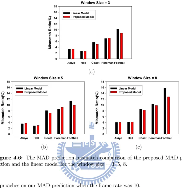
4.6 The MAD prediction mismatch comparison of the proposed MAD
pre-diction and the linear model for the window size = 3, 5, 8. . . 21
4.7 The average mismatch ratio of the MAD prediction in the window
size=3, 5, 8. . . 22
4.8 The QP prediction accuracy for the different window sizes. . . 23
4.9 The MAD mismatch distribution of the experiment 1 within the window
size = 3, 5, 8. . . 24
4.10 The performance of foreman sequence for the window size=3, 5, 8. . . . 25
4.11 The R-D performance comparison of Salesman sequence reconstructed by frame replication and frame interpolation based on the different
ob-jective quality measurement. . . 27
4.12 The performance comparison of Foreman sequence reconstructed by frame replication and frame interpolation based on the different
objec-tive quality measurement. . . 28
4.13 The performance comparison of Hall sequence reconstructed by frame replication and frame interpolation based on the different objective
qual-ity measurement. . . 29
4.14 The performance comparison of Football sequence reconstructed by frame replication and frame interpolation based on the different objective
CHAPTER 1
Introduction
1.1
Research Overview
Multimedia services such as surveillance, video-conferencing and media utilization are getting popular in recent years. Some of these applications require that the bit-rate and/or the decoded quality of video bitstreams satisfy certain constraints. For instance, the bit-rate may not exceed a target value due to the limitation on channel bandwidth, or there is a quality requirement for the coded frames. Within the extensive literature, however, comparatively little research has focused on the scenario where both the bit-rate and the distortion of the coded frames must be below a pre-determined level. In such a scenario, it is necessary to trade the temporal quality for the spatial quality, or vice versa, during the encoding. For doing so, a common technique is adaptive frame skipping.
1.2
Problem Statement
This thesis aims to develop a quality- and rate-constrained adaptive frame skipping scheme. Our objective is to determine which frames in a specified time window should
Sec 1.3. Contributions
be encoded and what the values of their quantization parameters (QP) are such that the following conditions are satisfied:
1. The bit-rate of the coded frames shall be less than a target value, 2. The distortion of each coded frame shall be below a given level,
3. When the skipped frames are interpolated, the overall distortion, including both the coded frames and the skipped ones, shall be minimized.
Stated in another way, our goal amounts to searching for the solution to the following constrained optimization problem:
[q∗, s∗] = arg min q,s N X i=1 Di(q, s) (1.1) s.t. N X i=1 Ri(q, s)≤ Rt and Di(q, s) ≤ Dmax,
where Di denotes the distortion of the i-th frame, Ri corresponds to the associated
number of coded bits; the vector s = [s1, s2, ..., sN] specifies the frame-skip pattern
with si = 1 indicating the skip of the i-th frame; q = [q1, q2, ..., qN] describes the
quantization parameters; and Rt and Dmax define the target bit-rate and the quality
requirement, respectively.
As can be seen from Eq. (1.1), the distortion constraints in our problem are
non-static: on one hand, the distortion of each coded frame has to be lower than Dmax, and
on the other hand, which frames deserve coding is not known in advance. For such a complex problem, there generally does not exist a closed-form solution. To solve the problem, dynamic programming can be used. Its computational complexity, however, increases exponentially with the number of frames contained in the window, making it unfeasible and unpractical for real applications. As a result, we proposed in this thesis a heuristic algorithm.
1.3
Contributions
In brief, our algorithm proceeds as follows:
1. Within a time window, we first compute all possible frame-skip patterns. 2. For each admissible skip pattern,
Chapter 1. Introduction
(b) We then use an R-Q model to estimate their coding bits.
3. For the skipped frames, we compute their distortions by conducting frame inter-polation.
4. Finally, we choose, among all possible frame-skip patterns, the one that has more non-skipped frames while satisfying both the rate and the quality constraints. Specifically, our main contributions in this work include the following:
• We proposed an empirical D-Q model based on the analysis of spatial-temporal frame complexity.
• We designed an adaptive frame skipping algorithm that uses the D-Q model, together with an R-D model, to determine the frame-skip pattern and the QP for the non-skipped frames.
• We also provided a detail analysis on how video content, distortion measures, and interpolation schemes may affect the frame selection and the reconstruction quality.
Experimental results indicate that our scheme has a significant improvement in R-D performance, as compared with the regular frame skipping and the other previous work. The improvement is most obvious in fast-motion sequences, and similar results are observed with the other objective measures, such as SSIM and VQM.
1.4
Organization
The remainder of this thesis is organized as follows: Chapter 2 contains a brief review of the related works and compares the problem settings of different schemes. Chapter 3 presents our adaptive frame skipping scheme and the proposed D-Q model. Chapter 4 provides simulation results and compares the performance of our scheme with that of the regular frame skipping and of the previous work. Finally, Chapter 5 summarizes our work and gives a list of future works.
CHAPTER 2
Background
2.1
Rate Control in H.264/AVC
Rate control plays an important role in the application of H.264. Rate control is employed to achieve good perceptual quality by regulating the variable bit rate output of video encoder to meet the target bit-rates and the user’s desired constraints. In general, rate control can be separated into two levels: the frame and the macroblock (MB) levels. One is frame level bit allocation which we examine in this thesis to handle the spatial and temporal quality of video effectively. The other is bit allocation in the macroblock level by effectively distributing bit budgets among MBs. Like H.263 and MPEG-4, H.264 allows variable frame skipping to keep the rate constraint. The goal of frame skipping control is to satisfy the target bit allocation. Further, in order to achieve optimal rate control scheme, the rate-distortion (R-D) model is usually used for modeling the encoded bits or the distortion. Consequently, the quadratic rate-quantization model of H.264 is briefly discussed in the section 2.2. Besides, a number of studies have investigated the rate control scheme in the different experiment conditions. So rate control via variable frame rate by R-D model or other approaches
Chapter 2. Background
are also discussed in the section 2.3.
2.2
Quadratic Rate-Distortion Model.
Rate control allocates a target number of bits to each frame and then computes QPs to meet the target bits. According to [1], a quadratic rate-distortion model was proposed as follows: Rtexture = µ c1 1 QP + c2 1 QP2 ¶ × A, (2.1)
where A is the mean of absolute difference of the residual component, QP denotes
the quantization parameter and ci denotes the model parameters that are fitted to the
data. Due to the fact that the actual MAD is not available before the QP calculation, the MAD of the coding unit can be predicted by the linear model as follows:
b
Al[i] = a× A[i − 1] + b, (2.2)
where bAl[i] presents the predicted MAD of frame i, A[i − 1] is the actual MAD at
the co-located position in the previous frame, a and b are two parameters that will be updated after coding each frame. In brief, Eq. (2.1) was used to compute the corresponding QP after the target number of bits for the frame is computed.
2.3
Related Works
Fixed frame skipping (FFS), adopted in H.264/AVC of the JM reference software, is one of frame skipping scheme to encode video for meeting the rate constraints. Be-cause it cannot flexibly select the frame to be coded and logically decide which frame should be dropped, some approaches such as adaptive frame skipping based on spatio-temporal complexity analysis have been proposed for solving the disadvantage of fixed frame skipping scheme. The related works about frame skipping scheme reported in the literature can be classified into two major categories. One is to adopt adaptive frame skipping based on spatio-temporal complexity analyses to achieve a good bal-ance between spatial quality and temporal quality for rate-distortion optimized video coding. The other is to consider the reconstruction of the skipped frame using
motion-Sec 2.3. Related Works
compensated frame interpolation at decoder and then to choose the dropped frame by modeling the reconstructed quality of the dropped frame using motion-compensated frame interpolation at encoder to meet the user’s requirements. In the following sec-tions 2.3.1 and 2.3.2, we reviewed some approaches that have been proposed for finding rate-distortion optimized video coding with frame skipping scheme.
2.3.1
Rate-Distortion Optimized Frame Skipping
Vetro et al.[2] proposed a video coding algorithm considering the trade-off between spatial and temporal quality. The purpose of the algorithm is to find the optimal frame rate and quantization parameter selection to minimize the mean square error with rate-distortion model and frame skipping control subject to constraints on the target bit-rate and buffer occupancy. This algorithm is based on analytical model that estimated the distortion of encoded frames and the distortion of skipped frames reconstructed from previous coded frame by using frame replication. But, the prediction accuracy of the distortion model is not sufficient, especially for the video sequence with mixed motion activity.
Song et al.[4] formulated the problem as a rate-distortion (R-D) optimization process and solved the problem by the gradient search in low bit-rate condition. The main idea is to predefine Lagrange multiplier and then to calculate the histogram of difference (HOD) of last two in the previous sub-GOP (12 frames as a unit) to estimate which frames to be encoded for the current sub-GOP. However, the approach presents a limited performance when the high motion and low motion are mixed among each sub-GOP because the frame rate of the current sub-GOP is predicted from the previous sub-GOP information and the variable frame rate can only be changed from one basic unit to another.
2.3.2
Interpolation-Quality-Oriented Frame Skipping
Kuo [5] provided a video coding algorithm based on estimating quality of skipped frames for deciding which frames to be coded in low bit-rate channel. He proposed a variable frame skipping scheme that introduced motion-compensated frame interpo-lation in the encoding process. The experiment results revealed the suitable frame skipping had generated the better PSNR quality than that of the conventional coding
Chapter 2. Background
with no frame skipping. Similar concept was also presented in Yang et al.[6], adaptive frame skipping, which is adopted in the video encoding process. Their algorithm was proposed based on a bidirectional motion estimation and adaptive overlapped block motion-compensated interpolation. Both of the two above-mentioned methods are used to model the reconstructed objective quality of the skipped frame using motion-compensated frame interpolation. However, the difference between them is the skipped frame selection strategy.
In summary, the previous studies were designed to determine the variable encoding frame rate through adaptive frame skipping scheme. The basic idea of adaptive frame skipping mechanism is to reduce bit usage in temporal domain and then the saved bits can be allocated to improve the spatial quality of video. Their scheme used the rate-distortion model and frame interpolation at encoder to estimate the objective quality of the dropped frame in the bit-rate constraint, respectively. However, no requirements for the objective quality of the coded frame have been considered. In the following, an adaptive frame skipping scheme subject to rate- and quality- constraint was proposed.
CHAPTER 3
Quality- and Rate-Constrained Frame
Skipping
3.1
Algorithm Overview
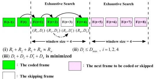
In Section 1.2, we discussed the problem of adaptive frame-skip coding with quality- and rate- constraints. In this chapter, we propose a frame selection scheme that adaptively skips frames based on a pair of R-Q and D-Q models, and provides a way to determine the quantization parameter for each coded frame. The notion of our algorithm can be expressed in Figure 3.1. In order to trade off processing delay and R-D performance, we first define a window size to specify the continuous number of frames that will influence the level of frame skipping (e.g., the window size in Figure 3.1 is equal to 4). Among the frames contained in the window, we search for a frame-skip pattern that yields the best reconstruction quality subject to a rate constraint, which is computed
as Rw = (Rb × Nw)/F with Rb, Nw, and F being the channel bandwidth, the number
of frames in the window, and the initial frame rate, respectively. An example of such a pattern is given in Figure 3.1, where the frame F(t+3) is skipped such that (i)
Chapter 3. Quality- and Rate-Constrained Frame Skipping F(t-1) F(t) F(t+1) F(t+2) F(t+3) F(t+4) F(t+5) window size = 4 ) , (R1 D1 (R2,D2)( ,R D3 3) ∗ ( , ) 4 4 D R 1 2 3 4 ( )i R +R +R +R ≈Rw ( )ii Di≤Dmax , i=1 2 4, , :The coded frame
:The skipping frame
:The next frame to be coded or skipped
F(t+6) F(t+7) F(t+8)
window size = 4 Exhaustive Search Exhaustive Search
1 2 3 4
( )iii D +D +D∗+D is minimized
Figure 3.1: The notion of the proposed algorithm. Note to graphics illustrator: (1)
The solid arrows indicate the path for estimating the bits and distortion of the coding frames by R-Q/D-Q models. (2) The dashed arrow indicates the reference frame used for frame replication.
R1+ R2+ R4 ' Rw, (ii) D1, D2, D4 ≤ Dmax, and (iii) D1+ D2+ D∗3+ D4 is minimized.
Remarkably, the D∗
3 represents the distortion (in mean squared error) of the skipped
frame F(t+3) when it is interpolated by replicating F(t+2). As will be seen in Section 4.1, the way in which the skipped frames are interpolated has an important effect on frame skipping.
In search of an optimal frame-skip pattern, it is necessary to acquire the rate Ri
and the distortion Di of each coded frame. Collecting the R-D data associated with
different frame-skip patterns actually requires coding the non-skipped frames. The complexity, however, may be so high that the approach becomes impractical. In order to reduce the computation, we employed a pair of R-Q and D-Q models that relate the estimated the rate and the distortion of each non-skipped frame to its quantization parameter. Unlike the conventional R-D models, ours allows the R-D estimation to be dynamically adapted to the change of the prediction distance. The design details are discussed in Section 3.2 and 3.3.
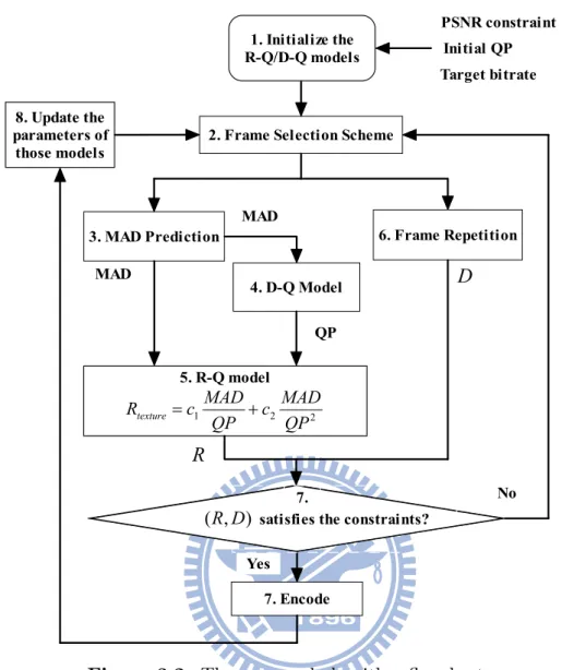
Figure 3.2 shows the flowchart of our algorithm, and the steps are as follows: Step 1 Initialize the R-Q and D-Q models.
Step 2 Compute all possible frame-skip patterns within the window. For example, if
the window size is 4, there are 24 frame-skip patterns.
Sec 3.1. Algorithm Overview 1. Initialize the R-Q/D-Q models 5. R-Q model 2 2 1 QP MAD c QP MAD c Rtexture= + ) , ( DR 8. Update the parameters of those models No Yes Target bitrate Initial QP PSNR constraint 7. Encode 4. D-Q Model 2. Frame Selection Scheme
3. MAD Prediction
QP MAD
6. Frame Repetition
satisfies the constraints? 7.
D
R
MAD
Figure 3.2: The proposed algorithm flowchart.
Step 3 Estimate the MAD of its prediction residues,
Step 4 Compute its QP with the D-Q model subject to the quality constraint, Step 5 Estimate the bit rate associated with the chosen QP using the R-Q model, Step 6 Measure the distortion of the skipped frame by assuming the use of frame
replication.
Among all plausible frame-skip patterns, we
Step 7 Choose the one that has more non-skipped frames while satisfying both the rate and quality constraints.
Step 8 Lastly, the R-D models are updated and (restarting from step 3) the process is repeated until the entire sequence is coded.
Chapter 3. Quality- and Rate-Constrained Frame Skipping
3.2
Distortion-Quantizer (D-Q) Model
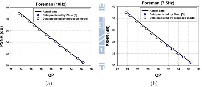
In our scheme, the QP for each non-skipped frame subject to the quality constraint must be determined. Therefore, a parametric model is needed to describe the relationship between the distortion and the QP of the non-skipped frames. Given the quality constraint (PSNR used as a measurement metric), the model can estimate the QP of the current frame based on the previous information (the distortion and the QP of the previous coded frame, etc.). Thus, we will adopt the D-Q model, proposed by Zhuo et al. [3], using a mathematical model to describe the relationships between the quantization parameter and the quality (PSNR used as a measurement metric) as follows.
P SN R = c1QP2+ c2QP + c3,
where QP denotes quantization parameter, P SN R denotes the reconstructed video
quality, and ci,i = 1, 2, 3 are model parameters.
However, the account of the effect of temporal complexity in the model, such as the sum or mean absolute differences of the residual component or the mean square error of the residual component on estimating the QP of the frame to be coded, is neglected. The prediction accuracy of the model can be critically influenced by the distance between the current frame and its reference. Accordingly, the impact of tem-poral complexity should be considered.
Based on our observations from a lot of experiment results which are generated by
using H.264 JM 12.3 [7], we find that the model is sensitive to | log 1
M AD|. In addition,
when the quantization step size and | logM AD1 | are used for the input parameters of
the model, the prediction accuracy of the model can be improved. So the quantization step size is used in place of the quantization parameter in the model. Therefore, the modified model can be formulated as follows:
P SN R = c1 µ¯¯¯ ¯log 1 M AD ¯ ¯ ¯ ¯ × Qstep ¶2 + c2 µ¯¯¯ ¯log 1 M AD ¯ ¯ ¯ ¯ × Qstep ¶ + c3,
where Qstep represents the quantization step size, M AD represents mean absolute
difference and ci,i = 1, 2, 3 denote the model parameters that are fitted to the data.
Sec 3.2. Distortion-Quantizer (D-Q) Model Foreman (10Hz) QP 22 24 26 28 30 32 34 36 38 P S NR (dB ) 30 32 34 36 38 40 Actual data
Data predicted by Zhuo [3] Data predicted by proposed model
Foreman (7.5HZ) QP 22 24 26 28 30 32 34 36 38 PSN R (dB ) 30 32 34 36 38 40 Actual data
Data predicted by Zhuo [3] Data predicted by proposed model
(a) (b)
Figure 3.3: PSNR-QP curves of Foreman sequence with regular frame skipping for
frame rate = 10, 7.5. Foreman (10Hz) QP 22 24 26 28 30 32 34 36 38 PSNR (dB) 30 32 34 36 38 40 Actual data
Data predicted by Zhuo [3] Data predicted by proposed model
Foreman (7.5Hz) QP 22 24 26 28 30 32 34 36 38 PS NR (d B) 30 32 34 36 38 40 Actual data
Data predicted by Zhuo [3] Data predicted by proposed model
(a) (b)
Figure 3.4: PSNR-QP curves of Foreman sequence with irregular frame skipping for
frame rate = 10, 7.5.
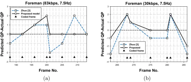
the proposed model data with regular and irregular frame skipping are shown in Figure 3.3 and Figure 3.4, respectively. Compare Figure 3.3 with Figure 3.4, the prediction accuracy of the two models are almost the same in sequential level. Therefore, the data in frame level are provided. As shown in Figure 3.5, the QP prediction error can be decreased substantially because the prediction distance between the current frame and its reference frame is taken into consideration in our model.
Chapter 3. Quality- and Rate-Constrained Frame Skipping Foreman (83kbps, 7.5Hz) Frame No. 190 195 200 205 210 Pre d ic te d Q P -A ct ual Q P -3 -2 -1 0 1 2 3 Zhuo [3] Proposed model Coded frame Foreman (30kbps, 7.5Hz) Frame No. 265 270 275 280 285 Pre d ic te d Q P -A ct ual Q P -4 -3 -2 -1 0 1 2 3 Zhuo [3] Proposed Coded frame (a) (b)
Figure 3.5: The QP prediction error traces of Foreman sequence for frame rate = 7.5
in bit-rate (a) 83kbps, (b) 30kbps.
3.3
Rate-Quantizer (R-Q) Model
In order to estimate the number of bits required for coding each non-skipped frame, we adopt the quadratic R-D model in Eq. (2.1), where the MAD is predicted linearly by
Eq. (2.2). Let cAL[i] denote the predicted MAD of frame i by the linear model. It has
been known that the linear MAD model performs poorly in video frames undergoing rapid temporal changes. For this reason, Liu et al. [8] proposed an adaptive MAD model that allows the MAD prediction to switch between the conventional linear model and their proposed direct model. Unlike the linear model, the direct model, as shown in Eq. (3.1), estimates the MAD of the frames to be coded.
c AD[i] = A[i− 1] × µ 1 + A[i− 1] A0[i− 1]× A0[i]− A0[i− 1] A0[i− 1] ¶ , (3.1)
where A0[i]is the MAD of the current frame i with zero motion, cAD[i]is the predicted
MAD of frame i by the direct model and A[i − 1] is the actual MAD of the (i − 1)-th frame resulting from motion-compensated prediction. They found that the actual MAD of the current frame can be estimated by the actual MAD of the previous reference frame and the prediction error was reduced by a weighting factor that includes the
previous known data since the fluctuation of A0[i] always reflects the fluctuation of
A[i].
Sec 3.3. Rate-Quantizer (R-Q) Model Coastguard (90kbps, 10Hz) O 5 10 15 20 25 30 A0 0 5 10 15 20 25 30 35 Football (152kbps, 10Hz) O 0 5 10 15 20 25 30 35 A0 0 5 10 15 20 25 30 35 (a) (b) Foreman (42kbps, 10Hz) O 0 10 20 30 40 A0 0 10 20 30 40 Salesman (20kbps, 10Hz) O 1 2 3 4 5 A0 3 4 5 6 7 (c) (d)
Figure 3.6: The relationships between O and A0 of (a) Coastguard, (b) Football, (c)
Foreman, (d) Salesman sequences.
the window, however, only the first frame within the window has the reconstructed reference frame and the actual MAD of the previous reference frame. In other words, the next frames within the window have no the above-mentioned the reconstructed
reference frame and the actual MAD except the current frame. Let cA0[i] and O[i]
denote the MAD of frame i when the previously-reconstructed frame and the previous source frame are used as the predictor, respectively. We expect O[i] between the current
frame i-th and the previous original frame (i−1)-th to be used to estimate cA0[i]because
their difference is only the quantization error. The linear relation between cA0[i] and
O[i]is justified by extensive experiments, with some of the results shown in Figure 3.6.
Therefore, the cA0[i] of the i-th frame is modeled by a linear predictor as follows:
c
Chapter 3. Quality- and Rate-Constrained Frame Skipping
where a and b denote the model parameters. Except the first frame in the window, the actual MAD of the remaining frames is unknown. For those frames, we modify the
direct model by using cA0[i] in place of A0[i] and using the predicted MAD instead of
the actual MAD. The Eq. (3.1) can be modified in the following:
c AD[i] = cAP[i− 1] × Ã 1 +AcP[i− 1] c A0[i] × Ac0[i]− cA0[i− 1] c A0[i− 1] ! , (3.2) where c AP[i− 1] = ⎧ ⎨ ⎩ c AL[i− 1] ΓL[i− 1] < ΓD[i− 1] c AD[i− 1] otherwise , ΓL[i] = i X n=0 ¯ ¯ ¯ cAL[n]− A[n] ¯ ¯ ¯ , ΓD[i] = i X n=0 ¯ ¯ ¯ cAD[n]− A[n] ¯ ¯ ¯ ,
where cAP[i] denotes the result which is adaptively switched between the linear model
and the direct model, ΓLand ΓD denote the similarity measure of the direct model and
the linear model, and i denotes the i-th frame within the window. Therefore, we use Eq. (3.1) to predict the first frame in the window and then use Eq. (3.2) to estimate others in the window.
CHAPTER 4
Experiments and Analyses
In this chapter, in order to evaluate the performance of the proposed coding method and to analyze the effects of the MAD and QP estimations on the frame selection scheme for the different window sizes, we conduct a set of experiments to illustrate:
1. To what extent the window size affects the accuracy of the MAD and QP esti-mations?
2. How the proposed scheme trades off the spatial and temporal quality?
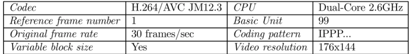
3. Which subjective quality assessment used to be the distortion measure is com-patible with human perceptional system in our experimental environment? We integrate the proposed algorithm into the H.264/AVC reference software, Joint Model version 12.3, to exhibit its utility. The details of the testing conditions in the following experiments are presented in Table 4.1.
4.1
Joint Spatio-Temporal Bit Allocation
In order to demonstrate the benefit of frame skipping in low bit-rate condition, we adopt H.264 JM reference software to encode video sequences in fixed frame skipping.
Chapter 4. Experiments and Analyses
Table 4.1: Testing conditions and encoder parameters
Codec H.264/AVC JM12.3 CPU Dual-Core 2.6GHz
Reference frame number 1 Basic Unit 99
Original frame rate 30 frames/sec Coding pattern IPPP...
Variable block size Yes Video resolution 176x144
Moreover, we use frame replication and motion-compensated frame interpolation to achieve a full frame rate video. For simplicity, we abbreviate frame replication as FR and motion-compensated frame interpolation as FI.
The five PSNR traces, indicating the qualities of full-frame-rate video reconstruc-tions up-converted from 30, 15, 10fps by FR and FI, are shown in Figure 4.1. From the figure, three important observations can be made:
1. Compare part (a) and (b). The performance of reconstructing frame-skipped videos by FR and FI are more effective than that of encoding videos with full frame rate in low bit-rate condition, especially for low motion sequences.
2. Compare the two frame interpolation schemes. The performance of motion-compensated frame interpolation is better than that of frame replication and the influence of motion-compensated frame interpolation on frame recover is more obvious than frame repetition, especially for high motion sequences.
3. Compare the PSNR with subjective quality. The distortion of skipped frames dominates the whole distortion of reconstructed frames which include non-coded frames, especially for high motion sequences.
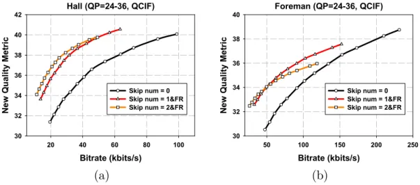
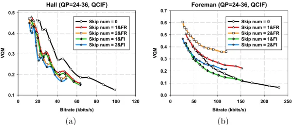
When we alter the quantization parameter and the frame rate simultaneously, the correlation between subjective quality and the PSNR become lower. For example, if we jointly change these two parameters, the PSNR may increase, whereas subjective quality may decrease. Therefore, in the following experiments, we will adopt various video quality assessments to demonstrate the benefit of skipped frame scheme in H.264. In addition to common objective quality measures, such as SSIM [9] and VQM [10][11], we also evaluate the performance by the new quality metric (NQM) [12] because it takes into account of the frame rate, motion speed and the PSNR. However, because NQM only considers the effect of frame replication in [12], we just use frame replication to reconstruct the skipped frames if we adopt NQM. Figure 4.2-4.4 present the rate-distortion curves of two different sequences in SSIM, NQM, and VQM, respectively.
Sec 4.1. Joint Spatio-Temporal Bit Allocation Hall (QP=24-36,QCIF) Bitrate (kbits/s) 20 40 60 80 100 PSNR-Y (dB) 30 32 34 36 38 40 Skip num = 0 Skip num = 1&FR Skip num = 2&FR Skip num = 1&FI Skip num = 2&FI
Foreman (QP=24-36,QCIF) Bitrate (kbits/s) 50 100 150 200 250 PSNR-Y (dB) 26 28 30 32 34 36 38 40 Skip num = 0 Skip num = 1&FR Skip num = 2&FR Skip num = 1&FI Skip num = 2&FI
(a) (b)
Figure 4.1: Rate-distortion curves of (a) Hall and (b) Salesman sequences for regular
frame skip number =0, 1, 2 in PSNR.
Hall (QP=24-36,QCIF) Bitrate (kbits/s) 0 20 40 60 80 100 120 SSI M 0.93 0.94 0.95 0.96 0.97 0.98 0.99 Skip num = 0 Skip num = 1&FR Skip num = 2&FR Skip num = 1&FI Skip num = 2&FI
Foreman (QP=24-36,QCIF) Bitrate (kbits/s) 50 100 150 200 250 SSI M 0.75 0.80 0.85 0.90 0.95 1.00 Skip num = 0 Skip num = 1&FR Skip num = 2&FR Skip num = 1&FI Skip num = 2&FI
(a) (b)
Figure 4.2: Rate-distortion curves of (a) Hall and (b) Salesman sequences for regular
frame skip number =0, 1, 2 in SSIM.
Hall (QP=24-36, QCIF) Bitrate (kbits/s) 20 40 60 80 100 Ne w Q u al it y M etr ic 30 32 34 36 38 40 42 Skip num = 0 Skip num = 1&FR Skip num = 2&FR
Foreman (QP=24-36, QCIF) Bitrate (kbits/s) 50 100 150 200 250 Ne w Q u al it y M etr ic 30 32 34 36 38 40 Skip num = 0 Skip num = 1&FR Skip num = 2&FR
(a) (b)
Figure 4.3: Rate-distortion curves of (a) Hall and (b) Salesman sequences for regular
Chapter 4. Experiments and Analyses Hall (QP=24-36, QCIF) Bitrate (kbits/s) 0 20 40 60 80 100 120 VQM 0.1 0.2 0.3 0.4 0.5 Skip num = 0 Skip num = 1&FR Skip num = 2&FR Skip num = 1&FI Skip num = 2&FI
Foreman (QP=24-36, QCIF) Bitrate (kbits/s) 0 50 100 150 200 250 VQM 0.0 0.1 0.2 0.3 0.4 0.5 0.6 0.7 Skip num = 0 Skip num = 1&FR Skip num = 2&FR Skip num = 1&FI Skip num = 2&FI
(a) (b)
Figure 4.4: Rate-distortion curves of (a) Hall and (b) Salesman sequences for regular
frame skip number =0, 1, 2 in VQM.
Comparing Figure 4.1 and Figure 4.2, we find that the R-D performance in PSNR and SSIM are similar, but on the contrary, there are very different trends between the performance in PSNR and NQM in comparison of Figure 4.1 with Figure 4.3. The main difference is that the performance of reconstructed frame-skipping video is more efficient than that of the encoding video with full frame rate. On the other hand, we also find that, as shown in Figure 4.4, the R-D performance in VQM is different from the R-D performance in PSNR because the former reflects the human visual system effectively.
4.2
Quality of the Proposed R-Q/D-Q Models
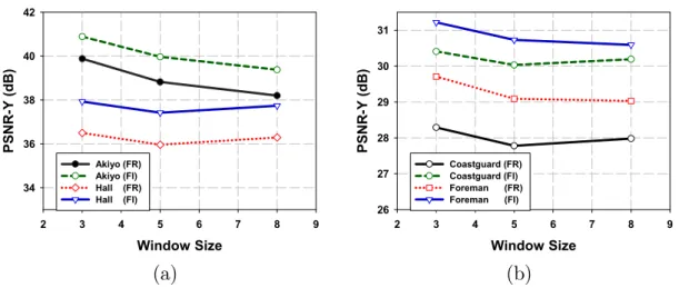
In order to analyze the effect of window size on the performance of our proposed scheme, we vary the window size in our experiments and observe the performance. Given the target bit-rates and PSNR constraints, then we encoded video sequences to obtain the PSNR-Y for the difference window sizes. It should be noted that the PSNR-Y is computed on the whole sequence including repeated frames. Figure 4.5 shows the experiment results, which indicate that the smaller the window size, the better the PSNR-Y performance. However, more frames will be predicted and considered when the window size increases. In the sections 4.2.1 and 4.2.2, we will analyze the possible factors that affect the performance for the different window sizes from the experiments.
Sec 4.2. Quality of the Proposed R-Q/D-Q Models Window Size 2 3 4 5 6 7 8 9 PSNR-Y (dB) 34 36 38 40 42 Akiyo (FR) Akiyo (FI) Hall (FR) Hall (FI) Window Size 2 3 4 5 6 7 8 9 PSNR-Y (dB) 26 27 28 29 30 31 Coastguard (FR) Coastguard (FI) Foreman (FR) Foreman (FI) (a) (b)
Figure 4.5: The average PSNR-Y comparison of the (a) slow motion sequences and
(b) high motion sequences for the window size=3, 5, 8.
4.2.1
MAD Prediction Accuracy
In this section, we analyze the effect of mismatch accuracy of our MAD prediction on the R-D performance. We carry out some experiments to compare our MAD prediction with the linear model. In our experiments, we examine the MAD prediction accuracy by using our MAD prediction for the window size = 3, 5, 8. Our MAD prediction and the linear model predict the same frames to be coded in the same conditions. In order to find the influence of variable frame rates and quantization parameters on MAD prediction, we evaluate the mismatch ratio between the predicted MAD and the actual MAD per frame, and we define
mismatch ratio(i) = A(i)b − A(i)
A(i) × 100%
where bA(i)is the predicted MAD of ith frame and A(i) is the actual MAD of ith frame.
Figure 4.6 shows the MAD prediction mismatches which are generated by the linear model and by our MAD prediction in the window size=3, 5, 8, respectively. Therefore, two observations can be made: (1) the bigger the window size, the lower the chance that it will accurately predict the actual MAD, and (2) the mismatch ratio of our MAD prediction is smaller than that of the linear model.
In order to analyze the factor that affects the MAD prediction accuracy, we set the following two experiments to find the influence of the different frame skipping
Chapter 4. Experiments and Analyses
Window Size = 3
Akiyo Hall Coast Foreman Football
Mi smatch Rati o( % ) 0 2 4 6 8 10 12 14 16 18 Linear Model Proposed Model (a) Window Size = 5
Akiyo Hall Coast Foreman Football
Mi smatch Rati o( % ) 0 2 4 6 8 10 12 14 16 18 Linear Model Proposed Model Window Size = 8
Akiyo Hall Coast Foreman Football
Mi smatch Rati o( % ) 0 2 4 6 8 10 12 14 16 18 Linear Model Proposed Model (b) (c)
Figure 4.6: The MAD prediction mismatch comparison of the proposed MAD
pre-diction and the linear model for the window size = 3, 5, 8.
approaches on our MAD prediction when the frame rate was 10. • Experiment 1: Fixed frame skipping (FFS) with fixed QP • Experiment 2: Variable frame skipping (VFS) with fixed QP
Note that variable frame skipping adopts the method which computes the mean square error (MSE) per two frames and then selects the frames to be coded with the highest MSE each three frames.
The comparison of the average mismatch ratio of the MAD prediction in the two experiment settings for the window size = 3, 5, 8 is shown in Figure 4.7. Two ob-servations could be extracted from Figure 4.7: (1) The mismatch ratio of the MAD prediction in experiment 1 is higher than that of experiment 2. VFS easily results in more frames skipped and hence the fluctuation of the MAD is so high that the estima-tion of the actual MAD becomes harder. (2) the larger the window size causes more frames to be predicted, and hence the mismatch ratio of the MAD prediction is larger.
Sec 4.2. Quality of the Proposed R-Q/D-Q Models
Window Size=3
Akiyo Hall Foreman Football
M ism atch Rati o 0 5 10 15 20 25 Experiment 1 Experiment 2 (a) Window Size=5
Akiyo Hall Foreman Football
Mi sm atch Ratio 0 5 10 15 20 25 Experiment 1 Experiment 2 Window Size=8
Akiyo Hall Foreman Football
Mi sm atch Ratio 0 5 10 15 20 25 Experiment 1 Experiment 2 (b) (c)
Figure 4.7: The average mismatch ratio of the MAD prediction in the window size=3,
5, 8.
4.2.2
QP Prediction Accuracy
In order to find the accuracy of the predicted QP by our proposed distortion model, we design the following experiment. The experiment can be described as following steps:
1. Encode a video sequence to get the PSNR and MAD of coded frames.
2. Use the PSNR and MAD from step 1 to estimate the QPs of coded frames by the proposed distortion model; in the meantime, the number of times predicted is based on the window size.
3. Compare the predicted QPs and the actual QPs to obtain the accuracy.
Figure 4.8 shows the results of the different sequences for the different window sizes. The details of the experiment results are presented in Table 4.2. From the figure and table, we found that when window size increased, the accuracy of predictive QPs decreased. Owing to the increase in the prediction distance between the predicted frame and the reference frame, the prediction error becomes larger.
Chapter 4. Experiments and Analyses Window Size = 1, 3, 5, 8 Window Size 2 4 6 8 A ccura cy 20 40 60 80 100 Akiyo Hall Coastguard Foreman Football
Figure 4.8: The QP prediction accuracy for the different window sizes.
Table 4.2: The accuracy of QP prediction of the differenet sequences for the different
window size.
Sequences window size = 1 window size=3 window size=5 window size=8
Foreman (15fps) 92.4% 56.6% 51.7% 51.7% Foreman (10fps) 96.8% 57.9% 48.4% 48.4% Football (15fps) 89.6% 61.6% 52.8% 47.2% Football (10fps) 89% 51.2% 34.1% 25.6% Hall (15fps) 91% 66.2% 56.6% 46.9% Hall (10fps) 89.5% 47.4% 50.5% 36.8% Akiyo (10fps) 93.7% 63.2% 48.4% 48.4% Akiyo (6fps) 94.5% 80% 80% 72.7% Coastguard (10fps) 93.7% 67.4% 62.1% 62.1% Coastguard (6fps) 83.6% 63.6% 49% 47.2% Pamphlet (10fps) 88.4% 55.8% 48.4% 37.9% Pamphlet (6fps) 89.1% 49.1% 50.9% 27.3% Salesman (10fps) 96.5% 76.4% 67.1% 66.2% Salesman (6fps) 97.6% 60% 60% 33.8%
Sec 4.3. Performance Evaluation
Figure 4.9: The MAD mismatch distribution of the experiment 1 within the window
size = 3, 5, 8.
4.2.3
Chain Effect of QP and MAD Prediction
In order to analyze the effect of MAD prediction error on our scheme, we survey the distribution of the MAD prediction mismatch ratio in experiment 1. Figure 4.9 shows the distribution results. In Figures 4.9, we find that the larger window size provides more flexibility in frame selection, but introduces more propagation errors. Because the actual MAD is not available during the frame selection, the prediction error chain effect results in the error propagation problem.
From Figure 4.5, we see that there are two factors that affect the performance for the different window sizes. One is the error propagation. The other is the window size. Figure 4.10 shows the performance of Foreman sequence for the different window sizes. In the figure, we find that the performance for the different window size are almost the same in low bit-rate coding. In addition, considering the human perceptional system, it is always better to avoid long runs of skipped frames, which may cause an undesirable visual effect. Based on the above-mentioned observations, no matter what the window size to be set ( we set to five here ), our scheme must at least encode one frame in the window.
4.3
Performance Evaluation
After the window size selection analyses have been studied in details, in this section, we evaluate the performance of our proposed scheme. We use
interpolation-quality-Chapter 4. Experiments and Analyses Foreman Bitrate (kbps/s) 60 80 100 120 140 160 180 PS NR-Y (dB) 26 28 30 32 34 36 Window Size = 3 Window Size = 5 Window Size = 8
Figure 4.10: The performance of foreman sequence for the window size=3, 5, 8.
oriented frame skipping (IFS) to select the coded frame and then meet the frame rate which we want. In addition, we know that the fixed frame skipping scheme (FFS) and variable frame skipping scheme (VFS) introduced in the previous section. The three schemes are used as baseline for comparison. The experiment process is as follows:
1. Set QP = 24.
2. Encode the test sequences with FFS, VFS, and IFS approaches at frame rate = 15, 10, 7.5, 6, respectively.
3. Obtain the distortion of the coded frames and the coded bit-rate and then mea-sure the distortion of reconstructed test sequences which include the skipped frame reconstructed by frame repetition or motion-compensated frame interpola-tion. This gives a particular combination of rate (R) and distortion (D), an R-D operating point.
4. Repeat step 2 and add 1 to QP until QP = 36.
5. Select the operating points that give the best rate-distortion performance (i.e. the lowest distortion for a given rate R) and then these operating points form a convex hull.
6. Use the smallest PSNR as quality constraint and the coded bit-rate as rate con-straint.
Through extensive experiments, we obtain the best R-D performance through the proposed scheme to compare the three schemes. Another objective quality measure-ment, such as SSIM, QM, and VQM, is adopted to evaluate the performance besides
Sec 4.3. Performance Evaluation
adopting the PSNR. The R-D performances of the different sequences are given in Figure 4.11-4.14, respectively. Therefore, from the figures, we can find that:
1. Compare the curves produced in the different quality assessments. As shown in Figure 4.11, we find that the R-D performance in PSNR and SSIM are similar, but on the contrary, there are very different trends between the performance in PSNR and NQM, especially for high motion sequences. On the other hand, all schemes show the similar performance with VQM.
2. Compare Figure 4.11(a) with Figure 4.11(e). We find that a tradeoff between spatial and temporal quality is limited in low bit-rate coding. In addition, by comparing Figure 4.12(a) with 4.12(e), we find that frame interpolation can im-prove more in FFS, VFS, and IFS. The main reason is more frames which are skipped in those schemes.
3. Compare the performances of four schemes in Figure 4.11. We find that the performance of the proposed method is superior to the performances of FFS, VFS, and IFS. The similar results can be found in Figure 4.12. Therefore, a good skipped frame selection is still needed.
Chapter 4. Experiments and Analyses
Salesman ( Frame Replication )
Bitrate (kbits/s) 10 20 30 40 50 PSNR-Y (dB) 28 30 32 34 36 38 40 FFS VFS IFS Proposed
Salesman ( Frame Replication )
Bitrate (kbits/s) 10 20 30 40 50 SSIM 0.82 0.84 0.86 0.88 0.90 0.92 0.94 0.96 0.98 1.00 FFS VFS IFS Proposed (a) (b)
Salesman ( Frame Replication )
Bitrate (kbits/s) 10 20 30 40 50 New Quality Me tr ic 28 30 32 34 36 38 40 FFS VFS IFS Proposed
Salesman ( Frame Replication )
Bitrate (kbits/s) 10 20 30 40 50 VQ M 0.0 0.1 0.2 0.3 0.4 0.5 0.6 FFS VFS IFS Proposed (c) (d)
Salesman ( Frame Interpolation )
Bitrate (kbits/s) 10 20 30 40 50 PSN R-Y (dB) 28 30 32 34 36 38 40 FFS VFS IFS Proposed (e) Salesman ( Frame Interpolation )
Bitrate (kbits/s) 10 20 30 40 50 SSIM 0.82 0.84 0.86 0.88 0.90 0.92 0.94 0.96 0.98 1.00 FFS VFS IFS Proposed
Salesman ( Frame Interpolation )
Bitrate (kbits/s) 10 20 30 40 50 VQ M 0.0 0.1 0.2 0.3 0.4 0.5 0.6 FFS VFS IFS Proposed (f) (g)
Figure 4.11: The R-D performance comparison of Salesman sequence reconstructed
Sec 4.3. Performance Evaluation
Foreman ( Frame Replication )
Bitrate (kbits/s) 40 60 80 100 120 140 PSNR-Y (dB) 24 26 28 30 32 34 36 38 FFS VFS IFS Proposed
Foreman ( Frame Replication )
Bitrate (kbits/s) 40 60 80 100 120 140 SSI M 0.70 0.75 0.80 0.85 0.90 0.95 FFS VFS IFS Proposed (a) (b)
Foreman ( Frame Replication )
Bitrate (kbits/s) 40 60 80 100 120 140 New Q u ali ty M etr ic 31 32 33 34 35 36 37 38 FFS VFS IFS Proposed
Foreman ( Frame Replication )
Bitrate (kbits/s) 40 60 80 100 120 140 VQM 0.1 0.2 0.3 0.4 0.5 0.6 0.7 FFS VFS IFS Proposed (c) (d)
Foreman ( Frame Interpolation )
Bitrate (kbits/s) 40 60 80 100 120 140 PSNR -Y ( d B) 24 26 28 30 32 34 36 38 FFS VFS IFS Proposed (e) Foreman ( Frame Interpolation )
Bitrate (kbits/s) 40 60 80 100 120 140 SS IM 0.70 0.75 0.80 0.85 0.90 0.95 1.00 FFS VFS IFS Proposed
Foreman ( Frame Interpolation )
Bitrate (kbits/s) 40 60 80 100 120 140 VQM 0.0 0.1 0.2 0.3 0.4 0.5 0.6 0.7 FFS VFS IFS Proposed (f) (g)
Chapter 4. Experiments and Analyses
Hall ( Frame Replication )
Bitrate (kbits/s) 20 25 30 35 40 45 50 PSNR -Y ( d B) 32 34 36 38 40 FFS VFS IFS Proposed
Hall ( Frame Replication )
Bitrate (kbits/s) 20 25 30 35 40 45 50 SSIM 0.950 0.955 0.960 0.965 0.970 0.975 0.980 FFS VFS IFS Proposed (a) (b)
Hall ( Frame Replication )
Bitrate (kbits/s) 20 25 30 35 40 45 50 New Q u ali ty M etr ic 36 37 38 39 40 FFS VFS IFS Proposed
Hall ( Frame Replication )
Bitrate (kbits/s) 20 25 30 35 40 45 50 VQ M 0.1 0.2 0.3 0.4 0.5 FFS VFS IFS Proposed (c) (d)
Hall ( Frame Interpolation )
Bitrate (kbits/s) 20 25 30 35 40 45 50 PSNR-Y ( d B) 32 34 36 38 40 FFS VFS IFS Proposed (e) Hall ( Frame Interpolation )
Bitrate (kbits/s) 20 25 30 35 40 45 50 SS IM 0.950 0.955 0.960 0.965 0.970 0.975 0.980 FFS VFS IFS Proposed
Hall ( Frame Interpolation )
Bitrate (kbits/s) 20 25 30 35 40 45 50 VQM 0.1 0.2 0.3 0.4 0.5 FFS VFS IFS Proposed (f) (g)
Figure 4.13: The performance comparison of Hall sequence reconstructed by frame
replication and frame interpolation based on the different objective quality measure-ment.
Sec 4.3. Performance Evaluation
Football ( Frame Replication )
Bitrate (kbits/s) 120 140 160 180 200 220 240 260 PSNR-Y ( d B) 22 24 26 28 30 32 FFS VFS IFS Proposed
Football ( Frame Replication )
Bitrate (kbits/s) 120 140 160 180 200 220 240 260 SS IM 0.60 0.65 0.70 0.75 0.80 0.85 FFS VFS IFS Proposed (a) (b)
Football ( Frame Replication )
Bitrate (kbits/s) 120 140 160 180 200 220 240 260 N ew Qua lit y Me tr ic 30.0 30.5 31.0 31.5 32.0 32.5 33.0 FFS VFS IFS Proposed
Football ( Frame Replication )
Bitrate (kbits/s) 120 140 160 180 200 220 240 260 VQM 0.30 0.35 0.40 0.45 0.50 0.55 0.60 FFS VFS IFS Proposed (c) (d)
Football ( Frame Interpolation )
Bitrate (kbits/s) 120 140 160 180 200 220 240 260 PSNR-Y ( d B) 22 24 26 28 30 32 FFS VFS IFS Proposed (e) Football ( Frame Interpolation )
Bitrate (kbits/s) 120 140 160 180 200 220 240 260 SSIM 0.60 0.65 0.70 0.75 0.80 0.85 FFS VFS IFS Proposed
Football ( Frame Interpolation )
Bitrate (kbits/s) 120 140 160 180 200 220 240 260 VQM 0.30 0.35 0.40 0.45 0.50 0.55 0.60 FFS VFS IFS Proposed (f) (g)
Figure 4.14: The performance comparison of Football sequence reconstructed by
mea-CHAPTER 5
Conclusions
In this thesis, we proposed an adaptive frame-skipping scheme which trades the tem-poral quality for the spatial quality, or vice versa, in order to satisfy both the rate and the quality constraints. Among the frames contained in a time window, our approach attempts to determine which should be encoded and what the values of their quanti-zation parameters are. For each admissible frame-skip pattern, its R-D performance is estimated through a D-Q model and a R-Q model, both specifically take into account the effects of frame skipping. As compared with the regular frame skipping and the other previous work, our scheme reveals a significant improvement in R-D performance, especially in fast-motion sequences. Similar results are also observed with the other objective measures, such as SSIM and VQM.
We plan to further extend our study in several directions: (1) to establish a theo-retical foundation for the empirical D-Q model, (2) to alleviate the error propagation in the prediction of the MAD and QP, and (3) to devise an adaptation scheme for the adjustment of window size.
Bibliography
[1] T. Chiang and Y.-Q. Zhang, “A New Rate Control Scheme Using Quadratic Rate-Distortion Modeling,” IEEE Trans. on Circuits and Systems for Video Technology, vol. 7, pp. 246 — 250, Feb. 1997.
[2] A. Vetro, Y. Wang, and H. Sun, “Rate-Distortion Optimized Video Coding Con-sidering Frameskip,” IEEE Int’l Conference on Image Processing, Oct. 2001. [3] L. Zhuo, X. G. Wang, Z. Wang, D. D. Feng, and L. Shen, “A Novel Rate-Quality
Model based H.264/AVC Frame Layer Rate Control Method,” Int’l Conference on Information Communications Signal Processing (ICICS), Dec. 2007.
[4] H. Song and C.-C. J. Kuo, “Rate Control for Low-Bit-Rate Video via Variable-Encoding Frame Rates,” IEEE Trans. on Circuits and Systems for Video Tech-nology, vol. 11, pp. 512 — 521, Apr. 2001.
[5] T. Y. Kuo, “Variable Frame Skipping Scheme Based on Estimated Quality of Non-coded Frames at Decoder for Real-Time Video Coding,” IEICE Trans. on Information and Systems, vol. E88-D, pp. 2849 — 2856, Dec. 2005.
[6] Y. T. Yang, Y. S. Tung, and J. L. Wu, “Quality Enhancement of Frame Rate Up-Converted Video by Adaptive Frame Skip and Reliable Motion Extration,”
BIBLIOGRAPHY
IEEE Trans. on Circuits and Systems for Video Technology, vol. 17, pp. 1700 — 1713, Dec. 2007.
[7] “H.264/AVC Reference Software JM12.3.” http://iphome.hhi.de/suehring/tml/. [8] Y. Liu, Z. G. Li, and Y. C. Soh, “Adaptive MAD Predication and Refined R-Q
Model for H.264/AVC Rate Control,” IEEE Int’l Conference on Acoustics, Speech and Signal Processing (ICASSP), May 2006.
[9] Z. Wang, H. R. S. A. C. Bovik, and E. P. Simoncelli, “Image Quality Assessment: From Error Visibility to Structural Similarity,” IEEE Trans. on Image Process, vol. 13, Apr. 2004.
[10] “ITS Video Quality Research.” http://www.its.bldrdoc.gov/n3/video/index.php. [11] M. Pinson and S. Wolf, “A New Standardized Method for Objectively Measuring Video Quality,” IEEE Trans. on Broadcasting, vol. 50, pp. 312 — 322, September 2004.
[12] R. Feghali, F. Speranza, D. Wang, and A. Vincent, “Video Quality Metric for Bit Rate Control via Joint Adjustment of Quantization and Frame Rate,” IEEE Trans. on Broadcasting, vol. 53, pp. 441 — 446, Sep. 2007.