APSK系統在長距離光纖通訊的理論探討及實驗

全文

(1)⊕ 國立中山大學光電工程研究所碩士論文. APSK系統在長距離光纖通訊的理論探討及實驗 Theoretical and experimental studies of the APSK format in long-haul optical fiber communication system. 研究生：吳俊億撰指導教授：多賀秀德. 中華民國九十七年六月.

(2)

(3)

(4) 誌謝非常感謝王朝盛老師跟孫迺翔老師在百忙之中抽空來幫我們口試，給我們寶貴的意見，讓本篇論文更加完整。在研究所接近兩年的生活裡，非常感謝多賀秀德老師的悉心指導。在實驗室相關事情的處理上，多虧了老師的意見，才能將事情順利的解決，也因此讓我學會了很多緊急應對的方法。在實驗上也非常感謝多賀老師的耐心與包容，耐心的回答我每一個問題以及聽我用破爛的英文表達我的想法。包容我的粗心大意，使得實驗室儀器壞了不少。我很榮幸能夠在老師的實驗室裡學習成長。另外也非常感謝張弘文老師，感謝老師上課的教學，讓我釐清了很多觀念，對於電磁理論有更深的一層瞭解，也非常感謝老師在我一年級時對我的照顧，我們沒有學長，很多事情都不清楚。學校行政方面還好有老師的幫忙與建議，讓我能夠順利的完成公文作業，也感謝老師每次都邀請我們一起去聚餐，讓我們能夠認識實驗室的人，跟老師有課業以外的交流，使我們感覺就像一家人。在實驗室的日子裡，平常有小賴、小華、老盧跟偉麒的陪伴，有不開心的時候也能互相鼓勵，遇到困難就互相幫忙，有了這群好朋友，研究生生活才能過的多采多姿。非常感謝心民學長，聊天時常常給了我很多意見，讓我對於未來不會太過迷惘，也常常聽我講實驗上的問題，給我一些建議讓我可以順利做完實驗。感謝先庸學長的指導，給了我不少建議，幫了我不少忙。感謝實驗室的伙伴：威彤跟勝軒，碩一一起完成了許多事情，一起幫忙老師建立了這個實驗室。也感謝實驗室的學弟彥廷、建霖、瑞軒跟博顥，有了新血的注入，實驗室更增添了活力，平常的課業討論不僅讓你們懂了很多東西，也讓我自己把以前不清楚的概念再重新複習了一遍，也多虧了你們幫忙處理事情，能夠讓我二年級時能專心做實驗完成自己的論文。感謝安立知公司周毓中先生的幫忙，沒有你的鼎力的協助，借給我們 BERTs，這篇論文也不可能順利的完成。感謝我的父母，辛苦的工作讓我可以無憂無慮的唸完研究所。雖然祝融無情的在去年五月降臨，幸好家人一切平安。雖然擔心家裡的狀況，父母仍然要我們安心的完成學業，不要為家裡的事情擔心。謝謝爸媽，我會好好努力報答您們的恩情。謝謝妹妹三不五時的噓寒問暖，讓我在實驗室累了的時候也能感到開心。最後感謝一直陪伴我的詠竹，妳的貼心讓我能把心專注在研究上，遇到困難時還有妳的鼓勵，陪我一起度過。感謝所有在我這兩年求學生涯中給予協助的人，有了你們的建議及協助，我才得以學習成長，走出自己的路。感謝你們！. 吳俊億 2008.06 于西子灣. I.

(5) 中文摘要在進階的調變系統中，強度和相位調變（Amplitude and Phase Shift Keying）系統相當的受人矚目，最主要的不外乎頻譜效率較高，可以有效的增加傳輸量。在現今的傳輸系統中，可利用的頻寬被光放大器限制著，如何在有限的頻寬中更加有效率的使用頻寬變成一個非常重要的議題。本論文著重於研究模擬以及實驗強度和相位調變(APSK)的傳輸表現。首先，我們做了一連串的模擬來探討理論分析。不論是強度調變（Amplitude Shift Keying）或者是相位調變（Phase Shift Keying）都會因為消光比（Extinction Ratio）的影響而使傳輸表現發生變化。本論文在此一部份探討了消光比對於APSK傳輸系統的影響，並且發現消光比的大小會對ASK及PSK的傳輸表現有反比的現象。換句話說，消光比大時，ASK的訊號比較好，PSK的訊號就會比較差。當消光比小時，ASK的訊號比較差，PSK的訊號就會比較好。為了要改進APSK的傳輸效率，本論文提出了一個方法改進傳輸效率，我們稱之為” Zero-nulling method”.這個方法改善了消光比造成傳輸表現反比的現象。並且我們利用模擬來證實了這個方法的可行性及是否有效率的增加。接下來，我們著手進行實驗的架構。本論文中架設了330公里長的傳輸光纖，利用這個架構來確認模擬的成果是否正確。我們用實驗確認了ASK及PSK 訊號傳輸上的表現，並且也確認了消光比對ASK及PSK訊號造成傳輸表現交易的影響。另一方面，本論文架設500公里公里長光纖來探討長距離APSK傳輸的表現，利用再迴圈系統（recirculating loop）可以得到光纖傳輸數千公里的傳輸表現，並且本利用此實驗架構來確認了”Zero-nulling method” 的可行性。. II.

(6) Abstract Amplitude and Phase Shift Keying (APSK) format is one of the most attractive advanced modulation formats because of its good spectral efficiency. As the information bandwidth of the current optical fiber communication system is limited by the optical amplifier bandwidth, it is important to utilize the limited bandwidth effectively. This master thesis focuses on to study the transmission performance of the APSK format both theoretically and experimentally.. At first, a theoretical study was conducted using a numerical simulation. As the Extinction Ratio (ER) of the Amplitude Shift Keying (ASK) signal affects the performances of both the ASK and the Phase Shift Keying (PSK) signals, the effect of the ER upon the transmission performance of the APSK format was studied. A clear trade-off between the performance of the ASK signal and the PSK signal due to the change of the ER was observed. Then, in order to improve the performance of the APSK format, a method to improve the transmission performance was proposed. This method was named as “zero-nulling method”, and it solved the trade-off issue caused by the ER. The effectiveness of this method was confirmed through the numerical simulation.. Next, an experimental study was conducted. An experimental setup including 330km optical fiber transmission line was prepared, and it was used to confirm the results of the theoretical simulation. The performance trade-off between the ASK and the PSK signals due to the ER was confirmed experimentally. Finally, another experimental study was conducted. An experimental setup of 500km transmission line was used for this study. By adopting the recirculating loop experimental setup, the transmission length could be extended to a few thousand kilometers. The applicability of the “zero-nulling method” was confirmed using this experimental setup.. III.

(7) ◎致謝..…………….…………………...…………………………..……… I ◎中文摘要…..……………….…..………………...………………..……. II ◎Abstract………………………………………..………...………....……III ◎List of Contents……………………………...……………….………… IV Chapter 1 Introduction............................................................................................................1 1.1 The background of optical fiber communication system.............................................1 1.2 Motivation of this thesis...............................................................................................2 1.3 The structure of this thesis ...........................................................................................3 Chapter 2 Simulation study of the APSK format using zero-nulling method ...................6 2.1 Introduction..................................................................................................................6 2.2 Simulation method of the APSK system .....................................................................6 2.2.1 APSK format.....................................................................................................6 2.2.2 Extinction Ratio ................................................................................................7 2.2.3 Method of simulation........................................................................................7 2.3 Simulation results of the APSK format and zero-nulling method .............................11 2.3.1 Simulation model of the APSK system........................................................... 11 2.3.2 Simulation results of the APSK transmission .................................................13 2.3.3 Zero-nulling APSK format..............................................................................14 2.3.4 Simulation results of the zero-nulling APSK transmission.............................15 2.4 Conclusion .................................................................................................................17 Chapter 3 Experimental investigation of APSK format focusing on extinction ratio .....18 3.1 Introduction................................................................................................................18 3.2 Experimental setup.....................................................................................................18 3.2.1 Transmitter ......................................................................................................19 3.2.2 Transmission line ............................................................................................19 3.2.3 Receiver ..........................................................................................................22 3.3 Results and discussions focusing on the effect of the ER..........................................23 3.3.1 Optical spectrum of the transmission line.......................................................23 3.3.2 Eye diagram of the ASK and the PSK signals................................................25 3.3.3 Performance of the ASK signal ......................................................................28 3.3.4 Performance of the PSK signal .......................................................................29 3.4 Conclusion .................................................................................................................30. IV.

(8) Chapter 4 Experimental investigation of the APSK format using zero-nulling method 31 4.1 Introduction................................................................................................................31 4.2 Experimental setup.....................................................................................................31 4.2.1 Experimental setup of the APSK system with the recirculating loop.............31 4.2.2 Recirculating loop...........................................................................................32 4.2.3 Setup to test the zero-nulling APSK system ...................................................34 4.3 Results and discussions..............................................................................................37 4.3.1 OSNR performance of the recirculating loop .................................................37 4.3.2 Performance of the long distance transmission ..............................................40 4.3.3 Performance of the APSK format using the zero-nulling method..................40 4.4 Conclusion .................................................................................................................43 Chapter 5 Discussion of simulation and experimental results...........................................44 5.1 Introduction................................................................................................................44 5.2 Discussion of the simulation results ..........................................................................44 5.3 Discussion of the experimental results ......................................................................46 5.4 Comparison of the results of the theoretical studies and the experimental investigations ...................................................................................................................54 Chapter 6 Conclusions...........................................................................................................56 List of abbreviations ..............................................................................................................58. V.

(9) Chapter 1 Introduction 1.1 The background of optical fiber communication system In recent years, the internet becomes very popular in the world. Everyone use internet to search the information they need. Therefore, the growth of the internet traffic is quite quick and the amounts of information flowing through the network become very huge. Under this situation, we need some systems to support the internet traffic. As the bandwidth of the electrical signal in the coaxial cable is limited, the electrical communication via the coaxial cable is not enough to support the internet. Therefore, the optical fiber communication system is required to support the huge communication traffic of the internet. As the optical fiber has the merit of low loss, the transmission distance can be extended relatively easily compared to the coaxial cable. After the development of the optical amplifiers, all-optical systems can be used in the long-haul optical fiber communication systems. There is no need to use Optical to Electrical (O/E) converters in the middle of the transmission line. All-optical system reduces the cost for the long-haul optical fiber communication systems, and it is useful for the undersea systems, for example. In recent years, Wavelength Division Multiplexing (WDM) has been developed very quickly as seen in table 1.1 [1], and the explosive growth of the transmission capacity is clearly observed. Figure1.1 illustrates the applicable area of the communication systems as a function of the transmission distance and the data rate [1]. As seen in the figure, there is virtually no limit of the transmission distance for the optical communication systems and the transmission capacity is higher than other transmission systems. The merits of the optical fiber communication systems are so clear that it covers all over the world both terrestrial and undersea.. Ref. [2] [3] [4] [5] [6]. Table 1.1 Examples of recent record fiber-optic transmission results Capacity×Distance Capacity Distance 1.3Pb/(s．km) 10.9Tb/s (273 ch× 40Gb/s) 117km 3.1 Pb/(s．km) 10.2Tb/s (256 ch×42.7Gb/s) 300km 36 Pb/(s．km) 6.0Tb/s (149 ch× 42.7Gb/s) 6,100km 10 Pb/(s．km) 2.6Tb/s (64 ch× 42.7Gb/s) 4,000km 16 Pb/(s．km) 1.6Tb/s (40 ch× 42.7Gb/s) 10,000km. 1.

(10) Fig. 1.1 Regeneration-free transmission distance versus data rate for various wireless and wired communication technologies [1]. 1.2 Motivation of this thesis Even though the optical fiber transmission system can provide a vast capacity, it is still not enough to support the growth of the internet traffic. If we want to increase the transmission capacity, the easiest way is to install a new system in the field. This is not a good idea because the installation cost will be expensive. A better choice will be to increase the transmission capacity of already installed system. As the information bandwidth of the current optical fiber communication system is limited by the optical amplifier bandwidth, it is important to utilize the limited bandwidth effectively. Therefore, the Dense WDM (DWDM) system is generally used for the long-haul system. The bandwidth is utilized more effectively compared to the Coarse WDM (CWDM) system because of the dense channel spacing. The channel spacing of the DWDM system is limited by a wide spectral width nature of the conventional Intensity Modulation Direct Detection (IM-DD) format. Therefore, advanced modulation format becomes a key to improve the transmission performance [7] and the spectral efficiency [8]. In the conventional binary modulation (1 bit/symbol), increase of the symbol rate is the only method to increase the transmission capacity. Increasing the signal symbol rate using the binary modulation format is difficult to achieve due to the electronic and the optical device speed limitation. Multi-level modulation format is an important technology because the spectral efficiency is higher than the conventional binary modulations. There are several 2.

(11) examples which focus on the multi-level modulation format. Recent activity shows 100-Gb/s transmission by using Differential Quadrature Phase Shift Keying (DQPSK) modulation format [9]. More advanced modulation formats are also studied like 50-Gb/s 32 Amplitude and Phase Shift Keying (APSK) for example [10]. The APSK format is one of the attractive modulation formats. There are several technical reports investigating the performance of the APSK format both theoretically and experimentally [11-13]. Even though, there are still not enough studies focusing on the APSK format, and the investigation of the APSK format has been conducted in this master thesis.. 1.3 The structure of this thesis This master thesis has six chapters. The first chapter is introduction. This chapter explains the background and the motivation of this thesis. Chapter 2 is the simulation study of the APSK format using the zero-nulling method. In this chapter, the simulation method and the simulation results of the APSK modulation format as a function of the Extinction Ratio (ER) is discussed. A method to improve the transmission performance of the APSK system is proposed in this chapter also. For chapter 3, the experimental study focusing on the effect of the ER in the APSK system is conducted. Chapter 4 is the experimental investigation of the long-haul optical fiber communication system using the APSK format. An experiment to confirm the method we proposed to improve the transmission performance of the APSK format is demonstrated in this chapter. In chapter 5, both numerical simulation and experimental investigation results are compared and discussed. Finally, this thesis is concluded in chapter 6.. 3.

(12) References in this chapter [1] P. J. Winzer, R. J. Essiambre, “Advanced Optical Modulation Formats,” Proc. of IEEE VOL.94, NO.5, pp.952-985, 2006 [2] K. Fukuchi, T. Kasamatsu, M. Morie,R. Ohhira, T. Ito, K. Sekiya, D. Ogasahara, and T. Ono, “10.92-Tb/s (273 × 40-Gb/s) triple-band/ultra-dense WDM optical repeatered transmission experiment,” Proc. Optical Fiber Communication Conf. (OFC), Paper PD24, 2001. [3] Y. Frignac, G. Charlet, W. Idler, R. Dischler, P. Tran, S. B. S. Lanne, C. Martinelli, G. Veith, A. Jourdan, J.-P. Hamaide, and S. Bigo, “Transmission of 256 wavelength division and polarization-division multiplexed channels at 42.7 Gb/s (10.2 Tb/s capacity) over 3× 100 km of TeraLight fiber,” Proc. Optical Fiber Communication Conf. (OFC), Paper FC5, 2002. [4] G. Charlet, E. Corbel, J. Lazaro, A. Klekamp, R. Dischler, P. Tran, W. Idler, H. Mardoyan, A. Konczykowska, F. Jorge, and S. Bigo, “WDM transmission at 6 Tbit/s capacity over transatlantic distance and using 42.7 Gb/s differential phase-shift keying without pulse carver,” Proc. Optical Fiber Communication Conf. (OFC), Paper PDP36, 2004. [5] A. H. Gnauck, G. Raybon, S. Chandrasekhar, J. Leuthold, L. S. C. Doerr, A. Agarwal, S. Banerjee, D. Grosz, S. Hunsche, A. M. A. Kung, D. Maywar, M. Movassaghi, X. Liu, C. Xu, X. Wei, and D. M. Gill, “2.5 Tb/s (64×42.7 Gb/s) transmission over 40×100 km NZDSF using RZ-DPSK format and all-Raman amplified spans,” Proc. Optical Fiber Communication Conf. (OFC), Paper FC2, 2002. [6] C. Rasmussen, T. Fjelde, J. Bennike, F. Liu, S. Dey, P. M. B. Mikkelsen, P. Serbe, P. V. der Wagt, Y. Akasaka, D. Harris, D. Gapontsev, V. Ivshin, and P. Reeves-Hall, “DWDM 40 G transmission over transpacific distance (10,000 km) using CSRZ-DPSK and enhanced FEC and all-Raman amplified 100 km Ultrawave fiber spans,” Proc. Optical Fiber Communication Conf. (OFC), Paper PD18, 2001. [7] T. Tsuritani, K. Ishida, A. Agata, K. Shimomura, I. Morita, T. Tokura, H. Taga, T. Mizuochi, N. Edagawa, and S. Akiba, “70-GHz-spaced 40 x 42.7 Gb/s transpacific transmission over 9400 km using prefiltered CSRZ-DPSK signals, all-Raman repeaters, and symmetrically dispersion-managed fiber spans,” IEEE J. of Lightwave Technol., VOL.22, NO.1, pp.215-224, 2004. [8] D. van den Borne, S. L. Jansen, E. Gottwald, P. M. Krummrich, G. D. Khoe, and H. de Waardt, ”1.5-b/s/HZ spectrally efficient 40 x 85.6-Gb/s transmission over 1,700 km of SSMF using POLMUX-RZ_DQPSK,” Proc. of Optical Fiber Communication Conf. (OFC), Paper PDP34, 2006. [9] M. Daikoku, I. Morita, H. Taga, H. Tanaka, T. Kawanishi, T. Sakamoto, T. Miyazaki, and T. Fujita, “100Gbit/s DQPSK Transmission Experiment without OTDM for 100G 4.

(13) Ethernet Transport”, IEEE J. of Lightwave Technol., VOL 25, NO.1, pp. 139-145, 2007. [10] N. Kikuchi, K. Mandai, K. Sekine and S. Sasaki, “First experimental demonstration of single-polarization 50-Gbit/s 32-level (QASK and 8-DPSK) incoherent optical multilevel transmission,” Proc. of Optical Fiber Communication Conference (OFC), Paper PDP21, 2007. [11] S. Hayase, N. Kikuchi, K. Sekine, and S. Sasaki, “Proposal of 8-state per symbol (binary ASK and QPSK) 30-Gbit/s optical modulation/demodulation scheme,” Proc. of European Conference of Optical Communication (ECOC), Paper Th2.6.4, 2003. [12] K. Sekine, N. Kikuchi, S. Sasaki, S. Hayase, C. Hasegawa and T. Sugawara, “40 Gbit/s, 16-ary (4 bit/symbol) optical modulation/demodulation scheme,” IEE Electron. Lett, VOL.41, NO.7, pp.430-432, 2005. [13] N. Kikuchi, K. Sekine, S. Sasaki, and T. Sugawara, “Study on cross-phase modulation (XPM) effect on amplitude and differentially phase-modulated multilevel signals in DWDM transmission,” IEEE Photon. Technol. Lett, VOL.17, NO.7, pp.1549–1551, 2005.. 5.

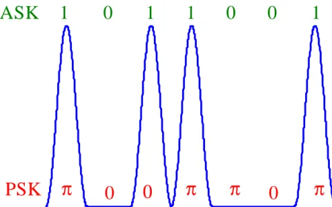
(14) Chapter 2 Simulation study of the APSK format using zero-nulling method 2.1 Introduction It is very important to investigate the possibility of conducting an experiment theoretically. Therefore, numerical simulations to investigate the performance of the APSK format are examined. In this chapter, the transmission performance of the APSK format in the long-haul optical fiber communication system is discussed. The simulation method used to simulate the transmission performance of the APSK system is explained in section 2.2. After that, the transmission performance of the APSK format is investigated focusing on the effect of the ER. Finally, in order to improve the transmission performance of the APSK system, a method named zero-nulling is proposed. The transmission performance of the proposed method is confirmed through numerical simulations.. 2.2 Simulation method of the APSK system In this section, the explanation of the APSK format and the simulation method to confirm the transmission performance of the APSK system is discussed. 2.2.1 APSK format Figure 2.1 shows a schematic diagram to explain the APSK format. When the ASK signal is transmitted, the PSK information is synchronously superimposed on the ASK signal, and the receiver receives two different information in one symbol. The bit patterns of the ASK signal and the PSK signal are independent. The spectral efficiency is doubled by this format compared to the original ASK format.. 6.

(15) ASK. 1. 0. 1. 1. 0. 0. 1. PSK. π. 0. 0. π. π. 0. π. Fig. 2.1 A schematic to explain the APSK format 2.2.2 Extinction Ratio The definition of ER is: ER =. The optical power of mark level The optical power of space level. (2.1). Figure 2.2 shows a schematic to explain the ER. Large ER means the difference between the mark level and the space level is large. Small ER means the difference between the mark level and the space level is small compared to the large ER case. In this thesis, the optical power of the mark level is fixed. Therefore, smaller ER case means the optical power of the space level is larger than that of the large ER case. ASK. 1. 0. 1. 1. 0. 0. 1. Mark level. Low ER. PSK. π. 0. 0. π. π. 0. π. Space level Fig. 2.2 A schematic explanation of the ER 2.2.3 Method of simulation Equation (2.2) shows the NonLinear Schrödinger (NLS) equation, which is used to evaluate the system performance in the optical fiber transmission.. 7.

(16) ∂A ∂A i ∂ 2 A α + β1 + β2 + A = iγ A2 A ∂z ∂t 2 ∂t 2 2. (2.2). γ stands for the nonlinear coefficient, and it is defined as γ = n2ω0/cAeff. A(z,t) is the slowing varying pulse envelope. β1 stands for the group velocity, and β2 stands for the group velocity dispersion. β2 is the first derivative of β1. α stands for the loss of the fiber. In general, time reference is set to move with the pulse at group velocity Vg, and the parameter t is transformed to a parameter T using equation (2.3).. T = t − z / Vg = t − β1 z. (2.3). Then, the equation (2.2) can be re-written as equation (2.4). ∂A i ∂2 A α (2.4) + β 2 2 + A = iγ A2 A ∂z 2 ∂T 2 This style is generally used, but equation (2.4) uses many approximations, and more generic. form of the NLS equation is shown in equation (2.5). ⎡ 2 ∂ A2 ∂A α i ∂ 2 A 1 ∂3 A i ∂ 2 + A + β2 2 − β3 3 = iγ ⎢ A A + ( A A) − RA ∂z 2 ∂T 2 ∂T 6 ∂T ω0 ∂T ⎢⎣. ⎤ ⎥ ⎥⎦. (2.5). R is the slope of the Raman gain. The NLS equation used for the simulation does not include the self-steepening term and the Raman term. Therefore, equation (2.5) can be re-written as equation (2.6), and this equation is used for the numerical simulation.. ∂A α i ∂2 A 1 ∂3 A + A + β2 2 − β3 3 = iγ ⎡⎣ A2 A⎤⎦ (2.6) ∂z 2 2 ∂T 6 ∂T There are several simulation methods that can be used to calculate the NLS. Most of them can be classified into two broad categories known as the finite-difference and pseudo-spectral method [1]. Generally speaking, pseudo-spectral method is faster by up to an order of magnitude to achieve the same accuracy. The split-step Fourier method is one of this method and has been used extensively to solve the pulse-propagation problem. There are several technical papers using the split-step Fourier method to investigate the transmission performance in the fiber [2,3]. Therefore, this method is used in this master thesis. Then, equation (2.6) can be written as ∂A ⎛ ^ ^ ⎞ = ⎜ D+ N ⎟ A ∂z ⎝ ⎠. (2.7). where. α. i ∂2 1 ∂3 D = − A − β2 + β3 2 2 ∂T 2 6 ∂T 3 ^. (2.8). ^. N = iγ ⎡⎣ A2 A⎤⎦. (2.9). and equation (2.6) can be solved as 8.

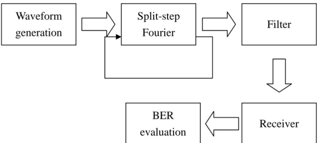
(17) ⎡ ^ ^ ⎤ A = A0 exp ⎢⎛⎜ D + N ⎞⎟ z ⎥ ⎠ ⎦ ⎣⎝. (2.10). ^. where D stands for the linear terms which includes the effects of the dispersion and the loss. ^. N stands for the nonlinear terms. Then, ^. ^. A( z + h,T ) = exp( h D )exp( h N ) A( z,T ). (2.11). Equation (2.11) represents the wave propagation in the fiber, which includes the effect of the linear term and the nonlinear term. It is difficult to calculate the linear term and the nonlinear term simultaneously with a long distance. Therefore, a method named split-step Fourier is used to calculate this equation. This method assumes small enough distance h so that the linear term and the nonlinear term can be calculated separately. At first, it is assumed that only the linear term affects to A(z,T), and A(z,T) becomes A’(z+h,T). Then, it is assumed that only the nonlinear term affects to A’(z+h,T) and obtains A(z+h,T). The operator is calculated by using the Fourier transform. Differentiation in time domain is converted to the imaginary frequency in the frequency domain using equation (2.12). ∂ = −iω ∂T. (2.12). Then, equation (2.8) in the frequency domain becomes ^. D=−. α 2. +. i i β 2ω 2 + β 3ω 3 2 6. (2.13). After calculating in the frequency domain, the inverse Fourier transform regenerate the waveform in the time domain. After that, the nonlinear term is calculated. This is one complete set of the calculation in a small distance h. Then, the procedure is repeated until the end of the transmission line. The simulation steps are explained briefly in figure 2.3. At first, the waveform of Pseudo Random Bits Sequence (PRBS) is generated by the waveform generator. The bit sequence is using a raised cosine waveform. After the signal generator, the split-step Fourier method is used to calculate the wave propagation in the system. The filter function is added before the receiver to reduce the Amplifier Spontaneous Emission (ASE) noise and separate the WDM signals. In the receiver, the optical pulse waveform is converted into the electrical pulse waveform. The Bit Error Rate (BER) is evaluated using the Q-factor calculated from the average and the distribution of the mark and the space levels of the received eye pattern.. 9.

(18) Waveform generation. Split-step Fourier. BER evaluation Fig. 2.3 Transmission simulation scheme. 10. Filter. Receiver.

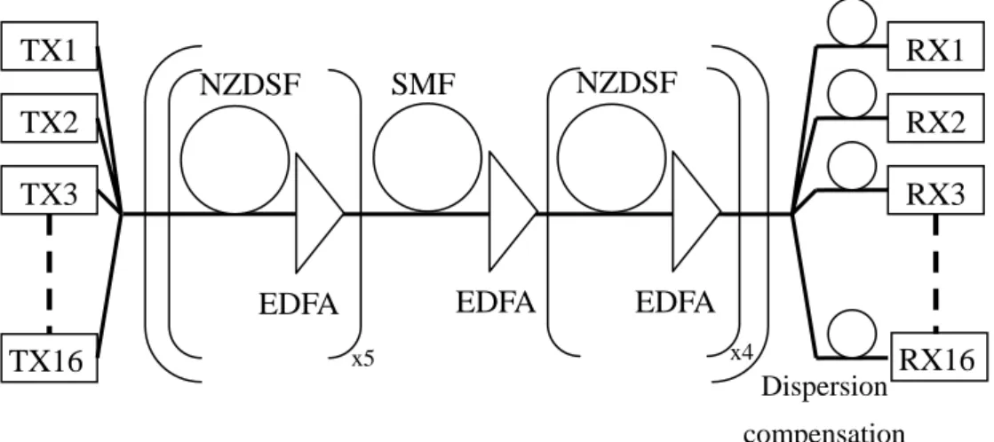
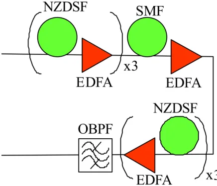
(19) 2.3 Simulation results of the APSK format and zero-nulling method The ER of the ASK signal affects the performance of both the ASK and the PSK signals. Therefore, the investigations of the APSK transmission performance as a function of the ER were conducted in this section. In addition, the method to improve the performance of the APSK format was proposed, and effectiveness of this method was confirmed through the simulations. 2.3.1 Simulation model of the APSK system In order to calculate the transmission performance of the APSK signal, following simulation model was utilized. Figure 2.4 shows a schematic diagram of the simulation model. The NLS equation was solved using the split-step Fourier method, which has already been explained in the previous section.. TX1. RX1 NZDSF. SMF. NZDSF TX2. RX2. TX3. RX3 EDFA. EDFA TX16. EDFA x4. x5. Dispersion. RX16. compensation. Fig. 2.4 A schematic diagram of the simulation model At the transmitter side, 16 modulated signals were used, and the signal wavelengths were ranged from 1545.5nm to 1554.5nm with 0.6nm channel separation. The modulation bit-rate and the pattern were 10Gbit/s and 29-1, respectively. There were 256 bits delay between the pattern for the ASK and that for the PSK in order to realize the pattern independence between the ASK signal and the PSK signal. The ASK signal had a Return to Zero (RZ) raised-cosine waveform. There was no wavelength selective function in the multiplexer. At the input of the transmission line, the pattern of all transmitters was synchronized to be the same. For the transmission line, a combination of the Non-Zero Dispersion Shifted Fiber (NZDSF) and the conventional Single Mode Fiber (SMF) was used. The parameters of the fibers were summarized in Table 2.1. There were ten fiber spans composed one block. The first to the fifth and the seventh to the tenth spans were the NZDSF, and the sixth span was the SMF. The repeater span length was 50km. The output power of each repeater was set to 11.

(20) +9dBm for 16 channels and the noise figure for the erbium-doped fiber amplifiers (EDFA) was 4.5dB. The wavelength dependent gain of the repeater was ignored. The cumulative Chromatic Dispersion (CD) for each channel after the transmission was fully compensated at the receiving end in order to clean up the linear waveform distortion due to the chromatic dispersion. Table 2.1: Parameters of the optical fibers Parameters. NZDSF. Chromatic dispersion (ps/km/nm) Dispersion slope (ps/km/nm2) Transmission loss (dB/km) Effective area (μm2) Nonlinear refractive index. SMF. -2 18 0.08 0.06 0.21 0.18 50 75 -20 2.6 x 10. The optical demultiplexer at the receiving end had the Gaussian shape. The bandwidth was 0.2nm. The ASK signal was directly detected by the optical receiver. The electrical bandwidth of the receiver was 7.5GHz, and the electrical filter shape was assumed to be the third order Bessel filter. The performance of the received signal was evaluated by the Q-factor. For the ASK signal, the amplitude of the photo current in the receiver was directly converted to the Q-factor. For the PSK signal, the calculation of the Q-factor was using the phase of the received signal [2]. Figure 2.5 shows the calculation method schematically. At first, the phase difference between zero and π was separated by one bit period, and the eye-like diagram in Fig. 2.5 was obtained. The time window was used to get the sampling point. The average and the standard deviation for π and zero were obtained from their distributions. Finally, the Q-factor is calculated using the formula (2.14). μ and σ in formula (2.14) are the average and the standard deviation, respectively, and π and 0 stands for the phase.. Fig. 2.5 Q-factor calculation using the phase difference. 12.

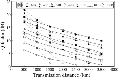
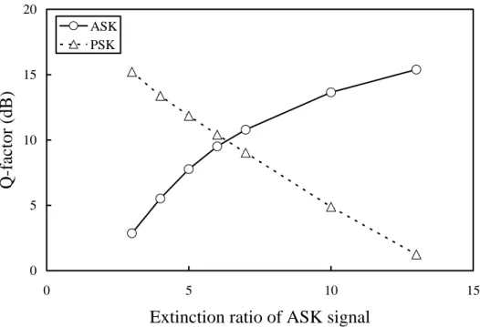
(21) Q=. μπ − μ 0 σπ +σ0. (2.14). 2.3.2 Simulation results of the APSK transmission Figure 2.6 shows the transmission performance of the APSK system. This figure shows the transmission performance of the ASK signal and the PSK signal as a function of the transmission distance and the ER of the ASK signal. Figure 2.7 shows the transmission performance after 1500km of the ASK and the PSK signals as a function of the extinction ratio of the ASK signal. Each point is an averaged value over 16 WDM channels for both figures. As shown in these figures, when the ER increased, the Q-factor of the ASK signal also increased. This means the performance became better when the ER increased. On the other hand, the performance of the PSK signal degraded as the ER increased. Figure 2.7 shows a clear trade off between the ASK signal and the PSK signal. As seen in this figure, the optimized point of the ER was around 5 to 6dB. It means the best ER for the APSK transmission system was 5 to 6dB.. 25. ASK PSK. 3dB. 4dB. 5dB. 6dB. 7dB. 10dB. 13dB. 20 15 10 5 0 0. 500. 1000. 1500. 2000. 2500. 3000. 3500. Transmission distance (km) Fig. 2.6 Transmission performance of the APSK signal. 13. 4000.

(22) 20 ASK PSK. Q-factor (dB). 15. 10. 5. 0 0. 5. 10. 15. Extinction ratio of ASK signal Fig. 2.7 Transmission performance of the APSK signal after 1500km 2.3.3 Zero-nulling APSK format As seen in the performance of the APSK system shown in the previous section, there is a clear trade off between the ASK signal and the PSK signal due to the ER of the ASK signal. The PSK signal suffers degradation when the extinction ratio of the ASK signal is large, and the reason of the degradation can be attributed to the PSK information in the space level of the ASK signal. The optical noise causes a significant degradation on this PSK information because the optical power is small. In order to improve the transmission performance, a method is proposed. As the PSK information in the ASK space level suffers significant degradation, if this PSK signal can be ignored, the transmission performance can be improved. Figure 2.8 shows an explanation of this method schematically. This method is named as “zero-nulling” method. The PSK information is carried only when the ASK signal is mark, and the PSK information is nulled while the ASK signal is zero.. 14.

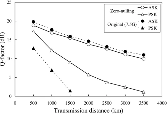
(23) (A) Original APSK (B) Zero-nulling APSK Fig. 2.8 A schematic to explain the zero-nulling method Because the PSK information is ignored on the ASK space level, and the mark ratio is one half in the general case, the capacity of the PSK signal becomes half compared to the original APSK format. As a result, the total effective bit-rate becomes 75% of that of the original APSK system. It is the trade off between this method and the original APSK system. Another issue of this method is that it is impossible to use the delay demodulation for the detection of the PSK signal. Still, it should be possible to utilize the homodyne/heterodyne detection with the digital signal processing [3] to obtain the phase information imposed only when the ASK signal is the mark. 2.3.4 Simulation results of the zero-nulling APSK transmission The effectiveness of the “zero-nulling” method was confirmed through the numerical simulations. The performance of the original APSK and the zero-nulling APSK was confirmed. As the total effective bit-rate was 75% of the original APSK system using the zero-nulling method, 7.5Gbits/s APSK system was acting as a reference to compare the performance of the APSK system using the zero-nulling method. The result is shown in figure 2.9. The extinction ratio of the ASK signal was set to 13dB for both the original and the zero-nulling APSK. As shown in this figure, the PSK signal had a significant improvement after using the zero-nulling method.. 15.

(24) 25 ASK PSK ASK PSK. Zero-nulling. Q-factor (dB). 20. Original (7.5G). 15. 10. 5. 0 0. 500. 1000. 1500. 2000. 2500. 3000. 3500. 4000. Transmission distance (km) Fig. 2.9 Transmission performance of the APSK signal with and without zero-nulling method. Figure 2.10 shows the phase eye diagrams after 1500km transmission. As shown in figure (a), the eye diagram was almost closed for the original APSK, but the eye in figure (b) was much clearly opened for the zero-nulling method. This result also shows the effectiveness of the zero-nulling method for the long distance transmission.. (a) (b) Fig. 2.10 Phase eye diagrams after 1500km transmission. (a) Original APSK, (b) Zero-nulling APSK. 16.

(25) 2.4 Conclusion In this chapter, the numerical simulation of the APSK format for the long-haul optical fiber transmission was conducted. It was observed that there was a clear trade off between the ASK signal performance and the PSK signal performance in the APSK system caused by the ER. It was found that the optimized point of the ER was 5 to 6dB after a few thousands kilometers transmission. In order to improve the transmission performance, the zero-nulling method was proposed. As seen in the numerical simulation results, the improvement was clearly observed by this method.. References in this chapter [1] G. P. Agrawal, Nonlinear Fiber Optics, Academic Press, 2001. [2] J. R. Costa, C. R. Paiva, and A. M. Barbosa, “Modified split-step Fourier method for the numerical simulation of soliton amplification in erbium-doped fibers with forward-propagating noise,” IEEE J. of Quantum Electronics, VOL.37, NO.1, pp.145-152, 2001 [3] O. V. Sinkin, R. Holzlöhner, J. Zweck, and C. R. Menyuk, “Optimization of the split-step Fourier method in modeling optical-fiber communications systems,” IEEE J. of Lightwave Technol., VOL.21, NO.1, pp.61-68, 2003 [4] X. Wei, X. Liu, and C. Xu, “Numerical simulation of the SPM penalty in a 10-Gb/s RZ-DPSK system,” IEEE Photon. Technol. Lett., VOL.15, NO.11, pp.1636-1638, 2003. [5] K. Kikuchi, “Phase-diversity homodyne detection of multilevel optical modulation with digital carrier phase estimation,” IEEE J. of Selected Topics in Quantum Electron., VOL.12, NO.4, pp.563-570, 2006.. 17.

(26) Chapter 3 Experimental investigation of APSK format focusing on extinction ratio 3.1 Introduction Following the theoretical investigation conducted in chapter 2, experimental investigation was carried out to confirm the results of the numerical simulation. This chapter focuses on the effect of the ER of the ASK signal in the APSK system. As discussed in chapter 2, there is a clear trade off between the ASK signal performance and the PSK signal performance in the APSK system through the ER. Therefore, purpose of this chapter is to confirm this trade off of the performance experimentally. Section 3.2 explains the experimental setup in detailed and shows the parameters of the transmission line. The transmission performance is briefly explained in section 3.3.. 3.2 Experimental setup In this section, the detail of the system setup is explained. Figure 3.1 shows a schematic diagram of the experimental setup. The explanation of the experimental setup is separated into three parts: the transmitter, the transmission line, and the receiver. The goal of this experiment is to clarify the effect of the ER in the APSK system, and to find out the optimized ER to get the best performance of the APSK system.. PPG RZ-Conv DFB-LD ASK ASK detector. EDL. NZDSF. SMF. x3. PSK. EDFA RX. EDFA NZDSF. OBPF. OBPF. EDFA. EDFA. Fig. 3.1 Schematic diagram of the APSK transmission system setup. 18. x3.

(27) 3.2.1 Transmitter Figure 3.2 is a schematic diagram of the transmitter. At the transmitter, there was a DFB-LD emitting at 1550.9nm, and an ASK modulator and a PSK modulator were connected in series after the Distributed FeedBack Laser Diode (DFB-LD). The ASK modulator was made from the LiNbO3 material and based on a Mach-Zehnder (MZ) interferometer [1,2]. The. Non-Return-to-Zero (NRZ) signal from the pulse pattern generator (PPG) was converted to the RZ format through the RZ converter, and it was fed to the ASK modulator. The PSK modulator was driven by another NRZ signal from the PPG. The reason of using the RZ format for the ASK signal was the limitation of the test equipment, because the ASK receiver only had the clock recovery function for the RZ signal. It was necessary to use the RZ format to retrieve the clock timing after the transmission, otherwise, the measurement of the BER might have some problems. An electrical delay line (EDL) was added between the PPG and the PSK modulator in order to synchronize the timing of the electrical signals to the ASK modulator and the PSK modulator. In order to adjust the ER of the ASK signal, the driving voltage and the bias voltage to the ASK modulator was controlled. The modulation bit-rate and the pattern were 10.66Gbit/s and 215-1, respectively.. Fig. 3.2 Schematic diagram of the transmitter. 3.2.2 Transmission line. Figure 3.3 shows a schematic diagram of the transmission line. Seven spans of the optical fibers and seven EDFAs were used for 330km transmission line. The optical fibers used for the experiment were the NZDSF and the SMF. The parameters of these fibers are summarized in Table 3-1. The NZDSF had a negative chromatic dispersion, and the SMF compensated the accumulated negative dispersion by its positive dispersion. The repeater span length of the NZDSF was 50km, while that of the SMF was 30km. The loss of each span was 11.5dB for the NZDSF and 7dB for the SMF. The dispersion map of 330km transmission line is shown in figure 3.4. The first to the third and the fifth to the seventh spans were the NZDSF, and the fourth span was the SMF. This kind of the dispersion map is commonly used for the under sea communication system. The averaged zero dispersion wavelength of 19.

(28) the transmission line was 1553.5nm. The EDFAs were used to compensate the loss of the fibers. The output power of the EDFA repeater was set to +3dBm. This was the optimized point that were tested. If the repeater output power was too small, the Signal to Noise Ratio (SNR) decreased. On the other hand, if the repeater output power was too large, it caused large nonlinear effect like a Brillouin scattering or a Self Phase Modulation (SPM). These nonlinear effects degraded the transmission performance. After the transmission line, an Optical Band Pass Filter (OBPF) was inserted to reduce the accumulated ASE noise of the EDFAs.. Fig. 3.3 Schematic diagram of the transmission line. Table 3-1 Parameters of the transmission fiber Parameters. NZDSF. SMF. Chromatic dispersion (ps/km/nm). -2. 20. Dispersion slope (ps/km/nm2). 0.128. 0.59. Transmission loss (dB/km). 0.23. 0.23. 20.

(29) cumulative dispersion(ps/nm/km). 400 200 0 -200. 330km. 0. 100. 200. 300. -400 distance(km) Fig. 3.4 Dispersion map of the transmission line. 21.

(30) 3.2.3 Receiver A schematic of the optical receiver is shown in figure 3.5. The EDFA acted as a preamplifier to improve the receiver sensitivity. The OBPF was used to reduce the ASE noise of the preamplifier. The coupler was used to split the optical power to the PDs (PD) of the ASK receiver and the PSK receiver. The ASK detector provided a recovered clock to measure the BER performance. The DPSK demodulator was used to demodulate the PSK signal. The Differential Phase Shifting Keying (DPSK) demodulator was using 1-bit delay scheme to switch the PSK information to amplitude signal. This amplitude signal was fed to the balanced PD. After that, the optical signal was converted to the electrical signal through this balanced PD. The PSK signal used the same clock to measure the BER performance, because the ASK signal and the PSK signal was synchronized. The performance of the ASK signal and the PSK signal was measured separately using this optical receiver.. Fig. 3.5 Schematic diagram of the receiver. 22.

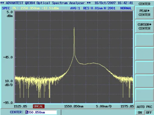
(31) 3.3 Results and discussions focusing on the effect of the ER 3.3.1 Optical spectrum of the transmission line The optical spectrum before transmission is shown in figure 3.6. The OSNR is 55dB at 0.01nm resolution. After 330km transmission, the ASE noise was accumulated. It is easy to observe this in figure 3.7. The ASE noise was generated by the EDFAs. As the signal power decreases after transmission through the optical fibers, the EDFAs are used to compensate the optical power to the next transmission stage, but the EDFAs not only increase the optical power of the signals but also add the optical noise. Therefore, the ASE noise accumulates in each repeater. After 330km transmission, the accumulated ASE noise power became significant, and if the PD received all of the noise power, the received signal was severely degraded. In order to overcome the degradation, the OBPF was used. As the OBPF did not remove the optical noise at the signal wavelength, the OSNR at the signal wavelength could not be improved by the OBPF. Without an OBPF, ASE noise of far apart from the signal wavelength could act as noise at the receiver, this ASE noise could be removed by the OBPF. Therefore, if we compare the performance without the OBPF, the OBPF improved the transmission performance. As shown in figure 3.8, the ASE noise far apart the signal wavelength was removed by the OBPF. It showed a clear optical spectrum compared to figure 3.7. Because another EDFA was added after the OBPF, the ASE noise in left side of the signal wavelength was increased as shown in figure 3.8.. Fig. 3.6 Optical spectrum before transmission. 23.

(32) Fig. 3.7 Optical spectrum after 330km transmission. Fig. 3.8 Optical spectrum after using OBPF. 24.

(33) 3.3.2 Eye diagram of the ASK and the PSK signals Figure 3.9 shows the electrical eye diagram of the ASK signal with different ERs for back-to-back and after 330km transmission. Because the electrical amplifier was included in the receiver, the electrical eye could not show the amplitude improvement clearly. As the ER increased, the eye opening became clearer in back to back situation. In the definition of ER, high ER means the difference between the mark level and the space level is large. Therefore, it is reasonable to observe a good eye opening in high ER case. After 330kmtransmission, the eye was degraded due to the accumulated ASE noise. It was expected that when the ER was small, the performance degradation due to the accumulated ASE noise was more significant compared to the high ER case. Even though the electrical amplifier affected the eye diagram shown in figure 3.9, the eye opening became clearer as the ER increased. For the PSK signal, the eye diagram is shown in figure 3.10. The eye became closed as the ER increased. The reason of this phenomenon can be attributed to the degradation of the PSK information in the ASK space level. The detailed explanation had mentioned in Chapter 2.2. After 330km transmission, the PSK signal suffered degradation due to the accumulated ASE noise, and it was clearly observed in the eye diagram after transmission.. 25.

(34) (a) back to back (ER 3dB). (c) back to back (ER 4dB). (e) back to back (ER 5dB). (b) after 330km transmission (ER 3dB). (d) after 330km transmission (ER 4dB). (f) after 330km transmission (ER 5dB). Fig. 3.9 Eye diagram of the ASK signal. 26.

(35) (a) back to back (ER 3dB). (c) back to back (ER 4dB). (e) back to back (ER 5dB). (b) after 330km transmission (ER 3dB). (d) after 330km transmission (ER 4dB). (f) after 330km transmission (ER 5dB). Fig. 3.10 Eye diagram of the PSK signal. 27.

(36) 3.3.3 Performance of the ASK signal Figure 3.11 shows the BER performance of the ASK signal. Figure 3.11 (a) shows the back-to-back performance and (b) shows the performance after 330km transmission. As seen in figure 3.11 (a), the performance of the ASK signal was improved when the ER was increased. The performance of the ASK signal after the transmission was degraded as shown in figure 3.11 (b). The reason of the degradation can be attributed to the ASE noise accumulation.. ER3dB ER3.5dB ER4.2dB ER5dB. -4. 10. -4. 10. -5. -6. -6. 10. 10. -7. -7. 10 -8 10 -9 10-10 10-11 10. 10 -8 10 -9 10-10 10-11 10 -37. -5. 10. BER. BER. 10. ER3dB ER3.5dB ER4.2dB ER5dB. -32. -27. -37. -22. RX Input Power (dBm) (a) back to back. -32. -27. (b) after 330km transmission. Fig. 3.11 Performance of the ASK signal. 28. -22. RX Input Power (dBm).

(37) 3.3.4 Performance of the PSK signal Figure 3.12 shows the BER performance of the PSK signal. Figure 3.12 (a) shows the back-to-back performance and (b) shows the performance after 330km transmission. As seen in the figure, the performance was degraded as the ER increased. As seen in figure 3.12 (b), the error floor was clearly observed when the ER was 5dB. According to the results of the ASK signal and the PSK signal shown in figure 3.11 and 3.12, high ER improved the transmission performance of the ASK signal, and degraded the performance of the PSK signal. On the other hand, the PSK signal had better performance in low ER case, but the performance of the ASK signal was degraded. Therefore, a tendency of the trade off between the ASK signal and the PSK signal was observed clearly.. 10. ER3dB ER3.5dB ER4.2dB ER5dB. -4. -4. 10. -5. -6. 10. -7. -6 -7. 10 -8 10 -9 10-10 10-11 10 -37. -5. 10. BER. BER. 10. 10. ER3dB ER3.5dB ER4.2dB ER5dB. 10 -8 10 -9 10-10 10-11 10 -32. -27. -22. -37. RX Input Power (dBm) (a) back to back. -32. -27. -22. RX Input Power (dBm). (b) after 330km transmission. Fig. 3.12 Performance of the PSK signal The power penalties at 10-9 BER as a function of the ER are shown in figure 3.13 The PSK signal could not achieve 10-9 BER when the ER was 5dB, so it was not plotted in the figure. As shown in this figure, the power penalties of the PSK signal increased as the ER increased. On the other hand, the power penalties of the ASK signal decreased as the ER increased. These results showed a clear trade-off between the ASK signal performance and the PSK signal performance of the APSK transmission.. 29.

(38) Power Penalty(dB). 4 ASK. 3. PSK. 2 1 0 2. 2.5. 3. 3.5. 4. 4.5. 5. 5.5. Extinction Ratio(dB). Fig. 3.12 Power penalty of ASK and PSK at BER=10-9. 3.4 Conclusion This chapter discussed the experimental investigation of the APSK system as a function of the ER. The transmission performance showed in this chapter demonstrated that high ER improved the transmission performance of the ASK signal and degraded that of the PSK signal. The PSK signal performance was improved when the ER was decreased. After the transmission, this tendency was clearer. These results show the clear trade off between the ASK signal performance and the PSK signal performance in the APSK system as expected from the theoretical study in chapter 2.. References in this chapter [1] G.. P. Agrawal, Fiber-optic communication systems, Wiley Interscience, Third Edition. [2] L. Thylen, “Integrated optics in LiNbO3: recent developments in devices for telecommunications,” IEEE J. of Lightwave Technol,. VOL 6, NO.6, pp.847-861, 1988.. 30.

(39) Chapter 4 Experimental investigation of the APSK format using zero-nulling method 4.1 Introduction This chapter focuses on the experimental investigation of the APSK system using the zero-nulling method. At first, the experimental setup of the recirculating loop is explained. This experimental setup is used to measure the performance of the long-haul optical fiber communication systems. After that, the experimental investigation focusing on the long-haul optical fiber communication system using the APSK modulation format as a function of the ER is discussed. Finally, the experiment of the APSK system using the zero-nulling method is conducted and the result is shown in section 4.3.3.. 4.2 Experimental setup 4.2.1 Experimental setup of the APSK system with the recirculating loop Figure 4.1 shows a schematic diagram of the recirculating loop setup. The experimental setup was almost the same with the previous experimental setup shown in chapter 3 except the transmission line and the wavelength of the DFB-LD. The wavelength of the DFB-LD was set to 1550.2 nm in order to reduce the Chromatic Dispersion (CD) in the transmission line. The length of the transmission line was increased to 500km in order to investigate the APSK system performance after long distance transmission. In addition, optical switch 1 and switch 2 were used to control the signal transmission through the optical fiber loop. Detail about the control of the recirculating loop is described in the next section. 31.

(40) PPG RZ-Conv DFB-LD. EDL EDFA OBPF Optical switch 1 Optical switch 2. NZDSF. x5. OBPF. SMF. x4. NZDSF. ASK detector. Fig. 4.1 Schematic diagram of the recirculating loop setup 4.2.2 Recirculating loop The recirculating loop experiment is very useful for evaluating the long-haul optical fiber communication systems. The length of the transmission line needed for the long-haul optical fiber communication system is a few thousand kilometers. It is very difficult to demonstrate this kind of the long transmission distance using straight line experimental setup. Therefore, the experimental setup of the recirculating loop is utilized to simulate the system performance of the long-haul optical fiber communication system.. Figure 4.2 shows the timing trigger of the recirculating loop. The unit period of the time is determined by the length of the transmission line. As the refractive index of the fiber is 1.475 and the speed of the light in vacuum is C=2.99792458*108(m/s), the light speed in the fiber C’ can be calculated as C’ =C/n (4.1) 8 C’=2.032491241*10 (m/s). As the fiber length L of the setup was 497.189055km, according to those parameters, the unit time period T to pass through the transmission line became T=L/C’ =2.446205155(ms) (4.2) Based on this calculation, the unit time period was determined. 32.

(41) The optical switch 1 in figure 4.1 turns on at the first period as shown in figure 4.2. The signal from the transmitter is transmitted to the transmission line and the receiver through 3dB coupler. At this moment, the receiver receives the signal that does not pass through the transmission line. In other words, the receiver receives the signal that performs under back to back situation. The same signal from another output from the 3dB coupler passes through the transmission line to switch 2, which turns on at the second period to let the signal passing through the 3dB coupler again. If the trigger to the error detector (ED) of the receiver turns on in this period like the red-solid line shown in figure 4.2, the ED can measure the transmission performance after the first loop. It means the measured performance is after 500km transmission when the red-solid line is used as the trigger to the ED. This signal not only transmits to the receiver, but also transmits to the transmission line again. Therefore, the switch 2 turns on at the third period to transmits the signal after the second round trip, and so on. As the figure 4.2 shows, the switch 2 turns on four units, it means this recirculating loop setup can transmit the signal over 2000km. The transmission distance can be increased as the periods of switch 2 are increased. The transmission distance is determined by number of recirculation through the loop. The actual distance to be measured is determined by the trigger position of the ED. As figure 4.2 shows, the performance of after 500km transmission can be measured when the red-solid line is used for the trigger of the ED, and the performance of after 1500km transmission can be measured when the blue-dotted line is used for the trigger of the ED. This is the operation principle of the recirculating loop.. 33.

(42) T SW1 time. SW2 time. ED time Fig. 4.2 Timing trigger of the recirculating loop 4.2.3 Setup to test the zero-nulling APSK system Figure 4.3 shows a schematic diagram to test the APSK system using the zero-nulling method. The experimental setup was almost the same as the experimental setup shown in chapter 3. The transmission distance was increased to 500km with 50km repeater span. The most important difference was the transmitter. Two individual PPGs were used to generate different signal patterns. The PSK signal was generated by a LiNbO3 phase modulator. The. modulation bit-rate and the pattern were 11.43Gbit/s and Pseudo Random Bits Sequence (PRBS) 215-1, respectively. The ASK signal was generated by a LiNbO3 MZ modulator. The modulation bit-rate was 11.43Gbit/s, and the test pattern was 32 bits sequence special pattern. This pattern had ten consecutive mark bits, ten consecutive space bits, and six consecutive mark and space bits pair like a schematic illustration shown in figure 4.4. The reason of using this kind of special pattern is explained in the next paragraph. The ASK modulator was driven by a RZ signal through a RZ converter, and the PSK modulator was driven by a NRZ signal.. 34.

(43) PPG RZ-Conv DFB-LD ASK ASK detector. PPG EDL. NZDSF. SMF. x5. PSK. EDFA RX. EDFA NZDSF. OBPF. OBPF. EDFA. EDFA. x4. Fig. 4.3 Schematic diagram for testing the zero-nulling method he zero-nulling method transmits the PSK information only when the ASK signal has a mark level. Therefore, if we can measure the BER of the PSK signal bit which corresponds to the ASK mark bit, we can evaluate the performance of the zero-nulling method experimentally. Therefore, a commercially available BER test set (Anritsu, MT1810A) was utilized to measure the performance of the zero-nulling method in the APSK system. The test equipment has 32 individual error counters, and the bit-error count is accumulated for each counter. This means that the BER can be measured by 32 different bit positions. The bit window measurement function enables or disables the BER measurement of a specific bit within these 32 bit positions [1]. The mechanism of the testing method is illustrated in figure 4.5. The squares with broad line in the figure are the chosen positions that will be ignored in the BER measurement. The BER test set can ignore any position in the 32 counters, and the testing position can be measured repeatedly to accumulate the bit errors in the counters. This is the reason why this experiment used the special 32 bits sequence for the ASK modulation. In the experimental setup, the bits position from 10 to 32 were chosen, which were ignored in the BER measurement. After that, the BER test set measure the BER performance of the PSK signal of the bits position from 1 to 9 which corresponds to the consecutive mark bits of the ASK signal.. 35.

(44) Fig.4.4 a schematic illustration of special testing pattern. 1. 2. 3. 4. …... 31. 32. 1. 2. 3. 4. …... 31. 32. 1. 2. 3. 4. …... 31. 32. 1. 2. 3. 4. …... 31. 32. -. 0. -. 0. 1. -. 0. …... 1. 0. 1. ….. 1. -. Fig. 4.5 A illustration of bit window. 36.

(45) 4.3 Results and discussions 4.3.1 OSNR performance of the recirculating loop The OSNR is confirmed in this section. The reason of testing the OSNR is that, if the OSNR is not correct in the transmission line, some issues cause degradation of the OSNR. To calculate the OSNR associated with a long-haul optical fiber communication system, the total ASE power needs to be calculated. The ASE power can be obtained using equation (4.3) [2].. PA S E = 2 n sp hν 0 N A ( G − 1) Δ ν o p t. (4.3). where 2nsp = Fn, Fn is the noise figure which is determined by the EDFA. h is Planck’s constant. ν0 is frequency of the signal. NA stands for the number of amplifiers. G is the gain of the amplifier. ΔνOPT is the bandwidth of the optical filter. The OSNR can be calculated using equation (4.3).. OSNR = Pin / PASE. (4.4). For the experiment, Fn of EDFA was 5dB, ν0 was 1550.1nm, N A was 11, G was 11.5dB, ΔνOPT was 0.2nm. According to those parameters, the OSNR was 27.8dB after 500km transmission. As shown in figure 4.6, the peak power after 500km transmission was -11.2dBm, and the noise level was about -39.7dBm .Therefore, the OSNR of the experiment was 28.5dB. The difference between the theoretical calculation and the experimental result was 0.7dB. It is small enough to say that the measured OSNR of 500km transmission agreed well to the theoretical calculation. At the third loop (1500km), the OSNR should be decreased by 4.8dB from the theoretical calculation because the number of the amplifiers became triple. The measured OSNR can be confirmed from figure 4.7. The peak power after 1500km transmission was -14.5dBm, and the noise level was -37.0dBm. Then, the measured OSNR was 22.5dB. The theoretical OSNR was 23.0dB. Therefore, the theoretical calculation and the experimental result were agreed well, and it was confirmed that there was no problem in the transmission line.. 37.

(46) (a) The optical spectrum with 10dB/division. (b) The optical spectrum with 0.5dB/division Fig. 4.6 OSNR after 500km transmission. 38.

(47) (a) The optical spectrum with 10dB/division. (b) The optical spectrum with 0.5dB/division Fig. 4.7 OSNR after 1500km transmission. 39.

(48) BER. 4.3.2 Performance of the long distance transmission At first, the transmission performance of the APSK system as a function of the transmission distance focusing on different ER of the ASK signal was measured. Figure 4.8 shows the results. A clear trade off between the ASK signal and the PSK signal in the APSK system was observed. This experimental result fits qualitatively well with the simulation results in chapter 2.. 10. -2. 10. -3. 10. -4. 10. -5. 10. -6. 10. -7. 10. -8. 10. -9. ASK. PSK. 0. 500. 1000. 1500. 2000. 2500. 3000. 3dB 4dB 5dB 6dB 10dB 3dB 4dB 5dB. 3500. Transmission distance (km) Fig. 4.8 BER as a function of the transmission distance 4.3.3 Performance of the APSK format using the zero-nulling method The performance of the zero-nulling method was evaluated after 500km transmission. Figure 4.9 shows the BER performance of the ASK signal in the APSK system as a function of the receiver input power with different ER. As seen in the figure, high ER showed better performance. After the transmission, the performance was degraded due to the ASE noise. The BER performance of the PSK signal in the APSK system is shown in figure 4.10. As shown in this figure, the BER performance of the PSK signal using the zero-nulling method was clearly improved regardless to the back to back situation and after 500km transmission, even when the ER was equal to 10dB.. 40.

(49) ER3dB ER4dB ER5dB ER6dB ER10dB. 10-4. BER. 10-5 -6. 10. -7. 10. 10-8 -9. 10 10-10 -11 10 -37. -32. -27. -22. -17. -12. -7. RX Input Power (dBm). (a) back to back ER3dB ER4dB ER5dB ER6dB ER10dB. 10-4. BER. 10-5 10-6 10-7 10-8 10-9 10-10 10-11 -37. -32. -27. -22. -17. -12. -7. RX Input Power (dBm). (b) after 500 km transmission Fig. 4.9 Performance of the ASK signal in the APSK system. 41.

(50) ER3dB ER4dB ER5dB ER6dB ZN(ER10dB). 10-3. BER. 10-4 10-5 10-6 10-7. 10-8 10-9 10-10 -37. -32. -27. -22. -17. -12. -7. RX Input Power (dBm). (a) back to back. ZN(ER10dB) ER=6dB. 10-3. 10-4. BER. ER=5dB. 10-5 10-6 ER=4dB. 10-7 10-8 10-9 10-10 -37. ER=3dB. -32. -27. -22. -17. -12. -7. RX Input Power (dBm). (b) after 500 km transmission Fig. 4.10 Performance of the PSK signal in the APSK system. 42.

(51) As shown in figure 4.10, the PSK signal using the zero-nulling method exhibited a clear improvement compared to the conventional APSK format. As mentioned in chapter 2, it is impossible to use the delay demodulation in this scheme, but a measurement technique using the delay demodulation was developed and the effectiveness of the zero-nulling method was confirmed experimentally. For the actual implementation of this method, it is needed to find some method to obtain the phase information imposed only when the ASK signal is equal to “one”.. 4.4 Conclusion The performance of the long-haul APSK system as a function of the ER was confirmed through the experiment in this chapter. A clear trade off between the ASK performance and the PSK performance was observed. The qualitative measurement of the zero-nulling method was conducted in this chapter, and the performance of the APSK system was clearly improved by using the zero-nulling method.. References in this chapter [1] Anritsu MU181040A Operation Manual [2] G. P. Agrawal, Fiber-optic communication systems, Wiley Interscience, Third Edition.. 43.

(52) Chapter 5 Discussion of simulation and experimental results 5.1 Introduction This chapter discusses the results obtained so far. At first, the results of the numerical simulations are discussed in section 5.2. Section 5.3 discusses the results of the experimental investigations. Some phenomenon shown in the experimental results are pointed out and discussed what kind of mechanism causes this kind of result. Section 5.4 compares the results of numerical simulations and experimental investigations. Some results of the experiments agree the numerical simulations, but some are not. The reasons of this kind of discrepancies are discussed in this section. 5.2 Discussion of the simulation results Figure 5.1 shows the simulation result of the transmission performance of the APSK signal as a function of the transmission distance with different ER of the ASK signal, which was already explained in chapter 2. As seen in this figure, the transmission performance degrades as the transmission distance extends. Because the chromatic dispersion was compensated by the dispersion map and the receiving terminal, the degradation was mainly due to the accumulated ASE noise. The accumulated ASE noise degraded the SNR, and the SNR degraded the transmission performance. Figure 5.2 summarizes the performance of the APSK signal after 1500km transmission. The ER was set from 3dB to 13dB. The transmission performance of the ASK signal became better when the ER increased, while the transmission performance of the PSK signal became better when the ER of the ASK signal decreased.. These results show a clear trade-off between the ASK performance and the PSK performance. The reason of the PSK performance degradation could be attributed to the degradation of the phase information in the space signal of the ASK format. In the definition, the optical power of the mark level was fixed. Therefore, high ER meant the optical power of the space level was small. As the space signal of the ASK format suffered the effect of the optical amplifier noise more severely, the information of the PSK format on this part was damaged, and the overall performance of the PSK signal was degraded. As shown in figure 5.2, the performances of the ASK signal and the PSK signal could be compromised. The optimum extinction ratio for 1500km transmission should be around 5 to 6dB.. 44.

(53) 25. ASK PSK. 3dB. 4dB. 5dB. 6dB. 7dB. 10dB. 13dB. 20 15 10 5 0 0. 500. 1000. 1500. 2000. 2500. 3000. 3500. 4000. Transmission distance (km) Fig. 5.1 Simulated transmission performance of the APSK signal. 20 ASK PSK. Q-factor (dB). 15. 10. 5. 0 0. 5. 10. 15. Extinction ratio of ASK signal Fig. 5.2 Simulated transmission performance of the APSK signal after 1500km transmission In figures 5.1 and 5.2, the performances of the APSK signal as a function of the ER and the transmission distance are described. Then, next step is the discussion of the zero-nulling method. Figure 5.3 shows the transmission performance of the APSK signal with and without the zero-nulling method. For the ASK signal, the performance of the original ASK signal (7.5G) was slightly better than the zero-nulling APSK because of the noise reduction 45.

(54) corresponding to the bit-rate reduction. The performance of 7.5G ASK signal was slightly better than 10G ASK signal. On the other hand, the PSK performance of the zero-nulling APSK signal was greatly improved compared to the original APSK signal. This simulation result showed that the zero-nulling method was proved to be quite effective to improve the long-distance transmission performance of the APSK format. On the other hand, because there was no PSK information in the ASK space level, the transmission capacity was reduced compared to the original APSK system. 25 ASK PSK ASK PSK. Zero-nulling. Q-factor (dB). 20. Original (7.5G). 15. 10. 5. 0 0. 500. 1000. 1500. 2000. 2500. 3000. 3500. 4000. Transmission distance (km) Fig. 5.3 Transmission performance of the APSK signal with and without the zero-nulling method 5.3 Discussion of the experimental results This section focuses on the results investigated experimentally. The phenomenon of the transmission performance is discussed in this section. Figure 5.4 shows the BER performance as a function of the transmission distance and the ER. As seen in this figure, the performance of the ASK signal was getting better as the ER was increased. On the other hand, the performance of the PSK signal was degraded as the ER was increased. This experimental result showed a clear trade off between the ASK signal and the PSK signal.. Next, the performance of the zero-nulling method was evaluated after 500km transmission. Because the bit window function was not compatible with the burst mode measurement required for the recirculating loop experiment, only the straight line transmission (500km) result was measured. Figure 5.5 shows the BER performance of the PSK signal in back to back situation and after 500km transmission. The performance was 46.

(55) BER. evaluated as a function of the ER of the ASK signal. As seen in figure 5.5(a), the performance of the PSK signal degraded as the extinction ratio was increased. It should be noted that the power penalty of 6dB ER case was the largest among five cases. When the ER was high, the PSK information in the ASK space level suffered significant degradation due to the small optical power.. 10. -2. 10. -3. 10. -4. 10. -5. 10. -6. 10. -7. 10. -8. 10. -9. ASK. PSK. 0. 500. 1000. 1500. 2000. 2500. 3dB 4dB 5dB 6dB 10dB 3dB 4dB 5dB. 3000. 3500. Transmission distance (km) Fig. 5.4 BER performance as a function of the transmission distance The performance after 500km transmission is shown in figure 5.5(b). The performance was degraded significantly compared to the back to back situation. Less than 10-9 BER could be achieved only when 3 dB ER case and with the zero-nulling method case. The error floor was clearly observed when the ER was 4, 5, and 6 dB. It could be explained that the PSK signal in the ASK space level suffered signal to noise ratio degradation due to the accumulated ASE noise, and it caused significant transmission penalty to exhibit an error floor after 500km transmission. As a matter of fact, we could only achieve synchronous loss both in back to back situation and after 500 km transmission when the extinction ratio was 10dB. On the other hand, we could achieve less than 10-9 BER even when the extinction ratio was 10dB with the zero-nulling method. From this result, it can be said that zero-nulling method was quite effective to improve the transmission performance of the APSK system.. 47.

(56) Figure 5.6 shows the eye diagrams of the PSK signal in different ER case. It was easy to observe the phenomenon of eye closure in high ER case. Those figures provided an evidence of the PSK information degradation in the ASK space level due to the small optical power. After the transmission, the degradation became more significant due to the accumulated ASE noise in the transmission line. When the ER was 10dB, the eye diagram was almost fully closed. This was the reason why we could only achieve synchronous loss both in back to back situation and after 500 km transmission when the extinction ratio was 10dB. Figure 5.7 shows the eye diagrams of the PSK signal with the zero-nulling method. These eye diagrams correspond to the special pattern of 32 bits sequence. As the pattern has ten consecutive mark bits, ten consecutive space bits, and six consecutive mark and space bits pair in the ASK signal, a clear eye opening of nine consecutive bits was observed in figure 5.7(a). In addition, an intermediate eye opening area was observed before the large eye opening area. As 1-bit delay demodulation scheme were used in this experiment, consecutive mark bits of the ASK signal showed the large eye opening area, and ten consecutive mark bits of the ASK signal corresponded to nine consecutive bits of the PSK signal after the demodulation. The intermediate eye opening area was generated by six consecutive mark and space bits pair in the ASK signal. Consecutive space bits of the ASK signal showed the worst eye opening area. Figure 5.7(b) shows the eye diagram after 500km transmission. Because the ASE noise caused significant signal to noise ratio degradation, only large eye opening area and no eye opening area were observed. Those figures also show the degradation of the PSK information in the ASK space level clearly.. 48.

(57) ER3dB ER4dB ER5dB ER6dB ZN(ER10dB). 10-3. BER. 10-4 10-5 10-6 10-7. 10-8 10-9 10-10 -37. -32. -27. -22. -17. -12. -7. RX Input Power (dBm). (a) back to back. ZN(ER10dB) ER=6dB. 10-3. 10-4. BER. ER=5dB. 10-5 10-6 ER=4dB. 10-7 10-8 10-9 10-10 -37. ER=3dB. -32. -27. -22. -17. -12. -7. RX Input Power (dBm). (b) after 500 km transmission Fig. 5.5 Performance of the PSK signal in the APSK system. 49.

(58) (a) ER 3dB, back to back. (b) ER 3dB, after 500km transmission. (c) ER 5dB, back to back. 50.

(59) (d) ER 5dB, after 500km transmission. (e) ER 6dB, back to back. (f) ER 6dB, after 500km transmission. 51.

(60) (g) ER 10dB, back to back. (h) ER 10dB, after 500km transmission Fig. 5.6 Eye diagram of the PSK signal in different ER. 52.

(61) (a)back to back. (b) after 500km transmission Fig. 5.7 Eye diagram of the PSK signal using zero-nulling method. 53.