國
立
交
通
大
學
電信工程研究所
碩 士 論 文
長期演進計畫系統下網路訊務之識別機制
Internet Traffic Identification Mechanism in LTE System
研 究 生:邱中玓
指導教授:李程輝 教授
長期演進計畫系統下網路訊務之識別機制
Internet Traffic Identification Mechanism in LTE System
研 究 生:邱中玓 Student:Chung-Ti Chiu
指導教授:李程輝 Advisor:Tsern-Huei Lee
國 立 交 通 大 學
電信工程研究所
碩 士 論 文
A ThesisSubmitted to Institute of Communications Engineering College of Electrical Engineering and Computer Engineering
National Chiao Tung University in partial Fulfillment of the Requirements
for the Degree of Master
in
Computer and Information Science
June 2011
Hsinchu, Taiwan, Republic of China
i
長期演進計畫系統下網路訊務之識別機制
學生: 邱中玓
指導教授:李程輝
國立交通大學電信工程研究所碩士班
摘
要
在長期演進技術 (LTE) 中,採用了非連續接收機制 (DRX) 去降低使用者的耗電 量。非連續接收機制的循環週期必須被設置能符合網路的訊務以至於達到最佳的 省電效應。如果沒有資料要傳送或接收,使用者將會關上傳送或接受器去省電。 在本論文中,我們提出了一種能去識別長期演進技術中網路訊務的方法。首先, 我們採用了支持向量機 (SVM) 去將網路訊務做分類。接著我們使用簡易突發性數 據分布 (bursty packet data distribution) 去模擬背景訊務,以及定義一個能偵測即時 訊息訊務的數值。最後我們提出了一種計算方法能識別背景訊務以及即時訊息訊 務的訊務特徵。模擬結果顯示出能用來代表線上訊務的數據。當我們不斷得到封 包的情況下,我們便不斷的更新這些數據,根據這些數據我們便能識別我們正在 使用的訊務狀況以及特徵。這機制可以提供一個方針給非連續接收機制的研究者 使用。 關鍵字: 非連續接收機制,支持向量機,突發性數據分布
ii
Internet Traffic Identification
Mechanism in LTE System
Student:Chung-Ti Chiu Advisor:Prof. Tsern-Huei Lee
Institute of Communications Engineering
National Chiao Tung University
ABSTRACT
Discontinuous reception (DRX) Cycle mechanism is adopted in Long Term Evolution (LTE) system to minimize the power consumption of user equipment (UE). DRX Cycle must be set to suit the Internet traffic to obtain the optimum performance for power saving. If there is no packet to transmit/receive, UE will turn off the transmitter/receiver based on DRX Cycle to reduce the power of UE. In this thesis, we proposed a mechanism to identify Internet traffic in LTE system. First, we adopted Support Vector Machine (SVM) algorithm for traffic classification. Then, we modeled Background traffic with a simplified bursty packet data distribution and defined a value to detect the use of Instant Message traffic. Finally, we proposed a method of calculation to recognize the characteristics of Background traffic and Instant Message traffic. Simulation results show the numerical parameters to represent on-line traffic. With these constantly updating parameters from the packets we captured, we can recognize the situation and characteristics of the traffic we are using. It provides a guideline for DRX researchers.
iii
誌
謝
非常感謝李程輝指導教授這兩年來辛苦的教導我許多做研究應該有
的態度以及方法。在這兩年的研究生活中,我學到許多專業知識和獨立思
考的能力,重要的是從老師身上學到了對研究及做事的正確價值觀。相信
在未來的道路上,這是一個非常棒的經驗。
感謝我的父母,邱潤文先生以及蕭瑞芳女士。謝謝他們對我的養育
之恩以及支持和鼓勵。也謝謝實驗室的學長姐及同學。咨翰、子竣、昌宏、
嗣儒、家安、冠佑的鼓勵及陪伴,讓我能順利的完成這兩年的學業。
最後謹將此論文獻給身邊所有愛我的人以及我愛的人。
iv
目
錄
中文摘要 i 英文摘要 ii 誌謝 iii 目錄 iv 圖目錄 v 表目錄 vi Chapter 1、 Introduction 1 Chapter 2、 Preliminary 4 2.1 DRX Mechanism 4 2.2 Traffic Identification 6
2.3 Support Vector Machine 10
Chapter 3、 Proposed Traffic Identification Mechanism 13
3.1 Characteristic of Background and Instant Message Traffic 13
3.2 Burst Traffic 20 3.3 System Model 22 Chapter 4、 Simulation 24 4.1 SVM Simulation 24 4.1.1 Features Selection 25 4.1.2 Accuracy of Prediction 26 4.2 Burst Simulation 29 4.2.1 Burst Definition 29
4.2.2 Bursty Traffic Distribution Parameters 31
4.3 Traffic Simulation 33
Chapter 5、 Conclusion 37
v
圖 目 錄
Figure 2.1
The DRX Cycle mechanism
5
Figure 2.2-(a) Packet size CDFs of Background traffic
9
Figure 2.2-(b) Packet size CDFs of Instant Message
9
Figure 2.3
The feature space in SVM
11
Figure 3.1-(a) The downlink trace of GPS
14
Figure 3.1-(b) The downlink trace of Facebook
15
Figure 3.1-(c) The downlink trace of weather
15
Figure 3.1-(d) The downlink trace of Network time
16
Figure 3.1-(e) The downlink trace of OS
16
Figure 3.2-(a) The uplink trace of GPS
17
Figure 3.2-(b) The uplink trace of Facebook
17
Figure 3.2-(c) The uplink trace of weather
18
Figure 3.2-(d) The uplink trace of Network time
18
Figure 3.2-(e) The uplink trace of OS
19
Figure 3.3
The CDFs of Instant Message traffic trace
20
Figure 3.4
Illustration of burst traffic.
21
Figure 3.5
system model
23
Figure 4.1
ratio of burst count with only one packet to burst amount
30
Figure 4.2-(a) The original Instant Message traffic
34
Figure 4.2-(b) The result after proposed traffic identification mechanism
34
Figure 4.3-(a) The original Background traffic
35
vi
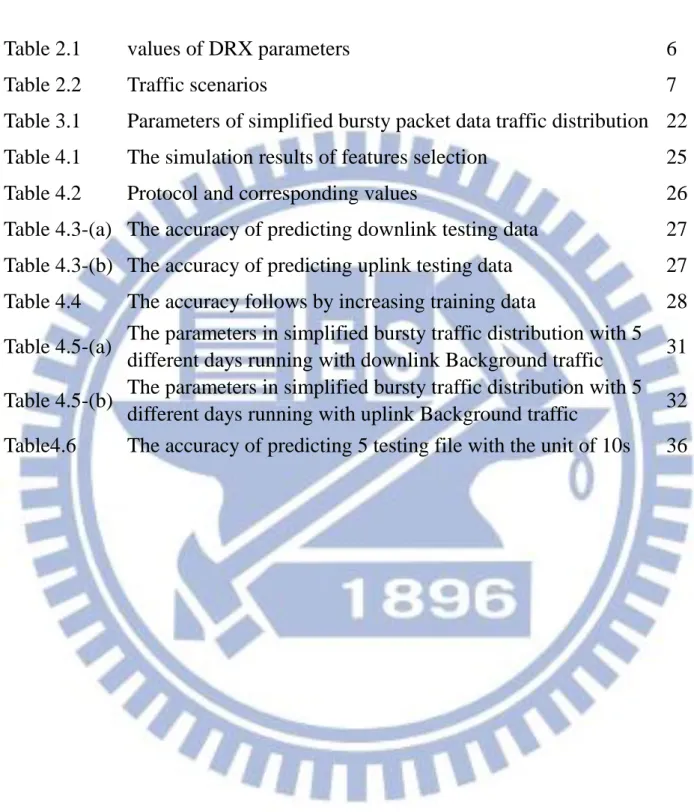
表 目 錄
Table 2.1
values of DRX parameters
6
Table 2.2
Traffic scenarios
7
Table 3.1
Parameters of simplified bursty packet data traffic distribution 22
Table 4.1
The simulation results of features selection
25
Table 4.2
Protocol and corresponding values
26
Table 4.3-(a) The accuracy of predicting downlink testing data
27
Table 4.3-(b) The accuracy of predicting uplink testing data
27
Table 4.4
The accuracy follows by increasing training data
28
Table 4.5-(a)
The parameters in simplified bursty traffic distribution with 5
different days running with downlink Background traffic
31
Table 4.5-(b)
The parameters in simplified bursty traffic distribution with 5
different days running with uplink Background traffic
32
1
Chapter 1.
Introduction
The wireless Internet service has greatly advanced in LTE. The power consumption of user equipment (UE) also increases because of the progress of the Internet data rate. Discontinuous Reception (DRX) mechanism is adopted in LTE system to decrease the power consumption of UE. The mechanism of DRX is a cycle that periodically turns UE into active mode or sleep mode [1]. The main DRX parameters are DRX Short Cycle, DRX Long Cycle, Inactivity timer, DRX Short Cycle timer, On duration timer. The mechanism of DRX cycle turns UE into sleep mode when UE does not receive any packets from Internet, and turns UE into active mode when UE captures a packet from Internet. The DRX Cycles must set to fit the on-line traffic so that we can obtain optimum power consumption. It means we should know the characteristics of traffic so that we can apply appropriate DRX parameters to particular traffic. Our purpose is to identify the on-line traffic in LTE.
3rd Generation Partnership Project (3GPP) is currently defining the traffic scenario in LTE system [2]. The traffic labels that 3GPP has defined currently are Background traffic, Instant Message, Gaming, Interactive Content Pull, and HTTP Video Streaming. Background traffic and Instant Message are discussed in the first place because of the characteristics of Background traffic and the widely using of Instant Message [3]. We only consider Background traffic and Instant Message in this thesis.
2
In this thesis, we want to classify the label of packets. We adopt Support Vector Machine (SVM) algorithm [4] to predict the label of packets. SVM is one of the machine learning algorithm using features for traffic classification. It was used to classify flows in previously Internet traffic [5]. The reason we adopt SVM is its high predicting accuracy and the rapid classifying time to classify data. We want to know what kind of traffic we are using right away, so we need the quality of rapid classifying time. Simulation results show the high predicting accuracy of SVM. We also find that with the features of packet size, protocol and source port number, we are able to classify packets into Background traffic or Instant Message with the predicting accuracy over 90%.
We observe the characteristics of Background traffic and Instant message form the traces we captured. Background traffic usually contains long fixed periods which follow by short bursts composed by packets. The long fixed periods vary from 500 seconds to 14400 seconds based on different applications. We model the Background traffic with a simplified bursty packet data traffic distribution [6]. With the parameters of simplified bursty traffic distribution from the on-line traffic, we can identify the characteristics of the traffic we are using. We also set a certain value to identify whether we are using Instant Message or not. We can roughly divide Internet traffic into background mode and active mode. In this thesis, active mode means we are running Instant Message. If we are not actively using mobile device, it means we are at background mode. We adopt minimum inter-packet arrival time, maximum inter-packet arrival time, average inter-packet arrival time, average packet size, average number of packets to describe the characteristics of active mode. We adopt average inter-burst idle time, average number of packets in a burst, average inter-packet arrival time in a burst to describe the characteristics of background mode.
3
The rest of this thesis is organized as follows. Chapter 2 briefly introduction the related works and techniques we are going to adopt for our system. The system model, problem formulation and proposed algorithms are introduced in chapter 3. The following chapter 4 gives the simulation. After that, a conclusion is drawn in chapter 5.
4
Chapter 2.
Preliminary
2.1
DRX Mechanism
According to the new generation of wireless network, the applications that people used in mobile devices are getting more complicated and more plentiful. This phenomenon also shows that the power consumption of the mobile devices becomes much higher than ever. To minimize the user equipment power consumption, a discontinuous reception mechanism has been adopted in LTE. There are five main parameters [7] in DRX mechanism as follows.
.DRX inactivity timer (TI) indicating the time in number of consecutive subframes
(without the scheduled traffic) to wait before enabling DRX. This timer is reset to zero and enabled immediately after successful reception of PDCCH (resource grant or allocation). When the timer reaches the advertised value for the radio bearer, the UE initiates the DRX.
.Short DRX Cycle (TDS) is the first DRX Cycle to be followed after enabling DRX.
.Long DRX Cycle (TDL) is the DRX cycle to be followed after TN DRX cycles.
.Short Cycle Timer (TN) is expressed in number of short DRX cycles. This parameter
indicates the number of initial DRX cycles to follow the short DRX Cycle before transitioning to the long DRX Cycle.
5
.On duration Timer (TON) is the number of frames over which the UE shall read the
DL control channel every DRX cycle before entering the power saving mode. TON is less than
TDS and TDL.
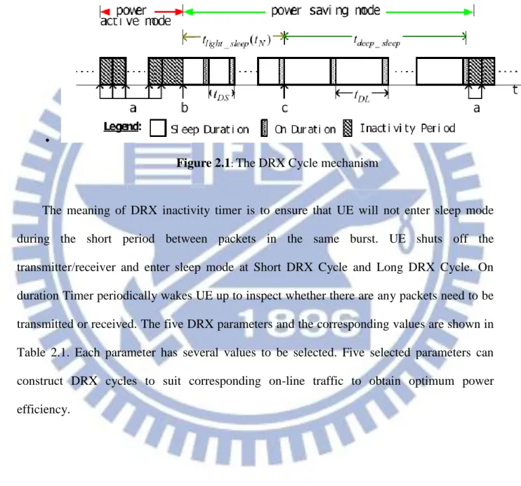
․
Figure 2.1: The DRX Cycle mechanism
The meaning of DRX inactivity timer is to ensure that UE will not enter sleep mode during the short period between packets in the same burst. UE shuts off the transmitter/receiver and enter sleep mode at Short DRX Cycle and Long DRX Cycle. On duration Timer periodically wakes UE up to inspect whether there are any packets need to be transmitted or received. The five DRX parameters and the corresponding values are shown in Table 2.1. Each parameter has several values to be selected. Five selected parameters can construct DRX cycles to suit corresponding on-line traffic to obtain optimum power efficiency.
6
Table 2.1: values of DRX parameters
DRX parameters values On duration Timer 1, 2, 3, 4, 5, 6, 8, 10, 20, 30, 40, 50, 60, 80, 100, 200 ms DRX inactivity timer 1, 2, 3, 4, 5, 6, 8, 10, 20, 30, 40, 50, 60, 80, 100, 200, 300, 500, 750, 1280, 1920, 2560 ms Short DRX Cycle 2, 5, 8, 10, 16, 20, 32, 40, 64, 80, 128, 160, 256, 320, 512, 640 ms Long DRX Cycle 10, 20, 32, 40, 64, 80, 128, 160, 256, 320, 512, 640, 1024, 1280, 2048, 2560 ms
Short Cycle timer Integer [1…16]
2.2
Traffic Identification
The types of Internet traffic in LTE are discussed in 3GPP Technical Specification Group Radio Access Network Working Group2 (TSG-RAN WG2). Table 2.2 shows the result they discussed so far. 3GPP working group decided to identify the characteristics of Background traffic and Instant Message first. The reason is that Background traffic is the most common traffic in mobile devices, and the amount of user using Instant Message increases rapidly. According this description in 3GPP, we only consider the traffic of Background and Instant Message in this thesis.
7
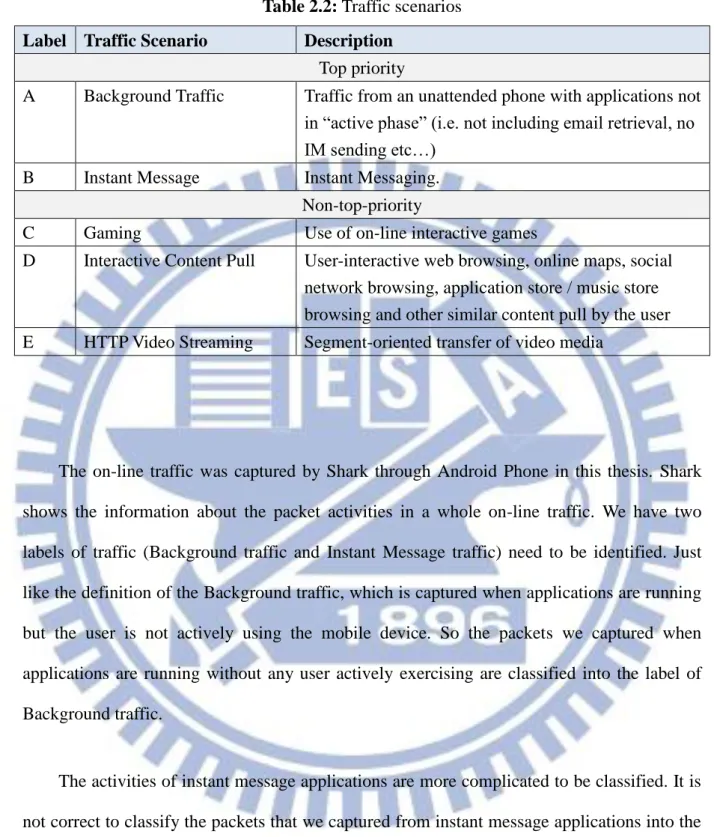
Table 2.2: Traffic scenarios Label Traffic Scenario Description
Top priority
A Background Traffic Traffic from an unattended phone with applications not in “active phase” (i.e. not including email retrieval, no IM sending etc…)
B Instant Message Instant Messaging.
Non-top-priority
C Gaming Use of on-line interactive games
D Interactive Content Pull User-interactive web browsing, online maps, social network browsing, application store / music store browsing and other similar content pull by the user E HTTP Video Streaming Segment-oriented transfer of video media
The on-line traffic was captured by Shark through Android Phone in this thesis. Shark shows the information about the packet activities in a whole on-line traffic. We have two labels of traffic (Background traffic and Instant Message traffic) need to be identified. Just like the definition of the Background traffic, which is captured when applications are running but the user is not actively using the mobile device. So the packets we captured when applications are running without any user actively exercising are classified into the label of Background traffic.
The activities of instant message applications are more complicated to be classified. It is not correct to classify the packets that we captured from instant message applications into the label of Instant Message, because instant message applications also produce background traffic [8]. We can categorize the traffic produced by instant message applications into user-related messages, heartbeat messages (keep alive), user status updating messages, others. User-related messages are produced when user sends/receives a message. Heartbeat messages
8
are periodic polling by the server to let server know that the user is still on-line. User status updating messages are produced when user changes the status or receives the update of friend status. We filter the packets of background traffic that instant message applications produce into the label of Background traffic, such as heartbeat messages. The packets captured when instant message applications are running but no user active using are classified into Background traffic. The packets captured when user send a message or receive a message are classified into Instant Message traffic. This kind of traffic includes user-related messages and user status updating messages. There are also some packets that are produced when no message exchanges but with user actively using (i.e. advertisement, download photograph of users…).The kinds of traffic are differ from the definition of Background traffic or Instant Message traffic, so we did not consider such kind of packets in this thesis.
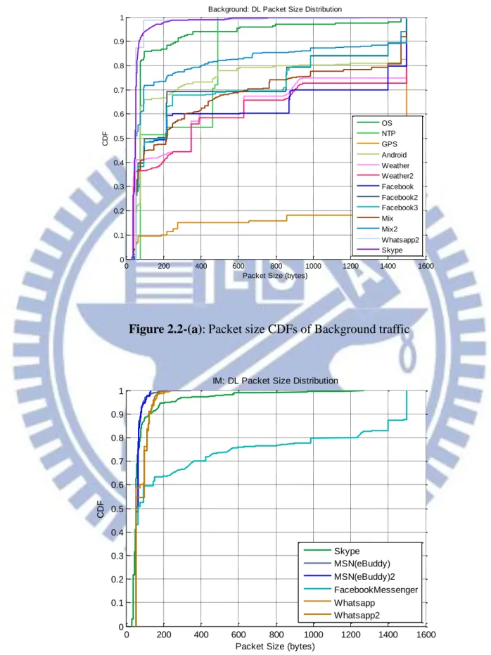
We can observe the difference about packet features between Background traffic packets and Instant Message packets from the trace files. The difference of packet size between Background traffic packets and Instant Message packets are shown in Figure 2.2-(a) and Figure 2.2-(b). The packet size of Background traffic varies from 68 bytes to 1516 bytes. The packet size of Instant Message principally varies from 68 bytes to 400 bytes. The protocols that Background traffic packets mostly adopt are TCP and UDP, but the Instant Message packets may adopt TCP, SSL and IMF. We also find the difference in source port number between the packets of Background traffic and Instant Message. Our observation shows that we can identify the packets from their packet features.
9
Figure 2.2-(a): Packet size CDFs of Background traffic
Figure 2.2-(b): Packet size CDFs of Instant Message
0 200 400 600 800 1000 1200 1400 1600 0 0.1 0.2 0.3 0.4 0.5 0.6 0.7 0.8 0.9 1
Packet Size (bytes)
CDF
Background: DL Packet Size Distribution
OS NTP GPS Android Weather Weather2 Facebook Facebook2 Facebook3 Mix Mix2 Whatsapp2 Skype 0 200 400 600 800 1000 1200 1400 1600 0 0.1 0.2 0.3 0.4 0.5 0.6 0.7 0.8 0.9 1
Packet Size (bytes)
CDF
IM: DL Packet Size Distribution
Skype MSN(eBuddy) MSN(eBuddy)2 FacebookMessenger Whatsapp Whatsapp2
10
2.3
Support Vector Machine
Support Vector Machine is a technique for data classification. SVM is one of the machine learning algorithms using flow features-based approach to classify. SVM requires training data to be labeled in advance and produces a model that fits the training data. Use the model to predict testing data, and compare the result of classification with the real label of testing data. The metric to measure this machine learning algorithm is the accuracy of prediction.
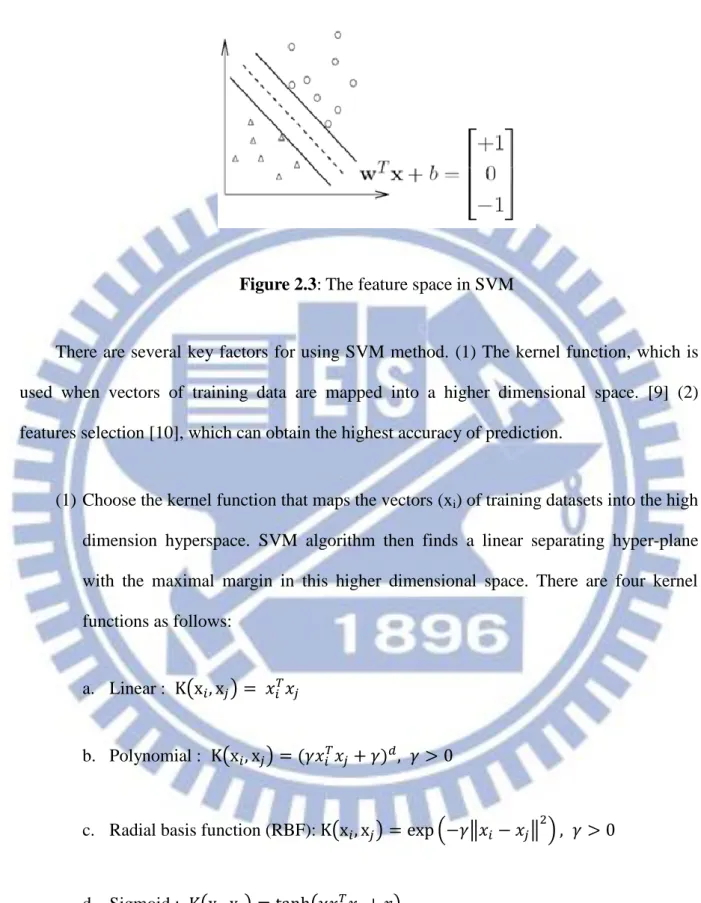
SVM means to acquire the information of data features and exchange into vectors in the feature space. The basic algorithm of SVM is to build the separating hyper-plane that
maximizes the distance between the specific regions that composed by the data for each label. The simplified illustration of SVM algorithm shows in Figure 2.3. Each point represents a data (packets are used in this thesis), the shape of each point is its label (only Background traffic and Instant Message traffic are considered in this thesis), and retrieve the information of features of each data to construct vectors in the feature space. After providing the training data to SVM, the feature space is constructed like Figure 2.3, and the algorithm will find the hyper-plane to distinguish the space built by the data with same label.
11
Figure 2.3: The feature space in SVM
There are several key factors for using SVM method. (1) The kernel function, which is used when vectors of training data are mapped into a higher dimensional space. [9] (2) features selection [10], which can obtain the highest accuracy of prediction.
(1) Choose the kernel function that maps the vectors (xi) of training datasets into the high
dimension hyperspace. SVM algorithm then finds a linear separating hyper-plane with the maximal margin in this higher dimensional space. There are four kernel functions as follows:
a. Linear : K(x𝑖, x𝑗) = 𝑥𝑖𝑇𝑥𝑗
b. Polynomial : K(x𝑖, x𝑗) = (𝛾𝑥𝑖𝑇𝑥𝑗+ 𝛾)𝑑, 𝛾 > 0
c. Radial basis function (RBF): K(x𝑖, x𝑗) = exp (−𝛾‖𝑥𝑖 − 𝑥𝑗‖2) , 𝛾 > 0
d. Sigmoid : K(x𝑖, x𝑗) = tanh(𝛾𝑥𝑖𝑇𝑥𝑗 + 𝑟)
We choose the RBF kernel function. This kernel function nonlinearly maps data into a higher dimension space, so it can handle the situation when the relation between the
12
labels and features are nonlinear. Another reason is the complexity which produced from the parameters of the kernel function is less than Polynomial and Sigmoid kernel functions. The RBF kernel function also has fewer numerical difficulties than Polynomial and Sigmoid kernel functions. In general, the RBF kernel function is the first choice.
(2) Features selection not only decides the degree of the feature space but also the complexity that may influence the accuracy of prediction. So it is necessary to find the appropriate combinations of features that have great positive effect on the performance of prediction. There are several features selection method as follows:
a. Optimum searching method means to exhaust all possible combinations and then find a best combination of features that can obtain best performance of prediction. The advantage of using this method is that we can find the best combination, but also has great complexity of calculation. If we have n features to select, we must have 2n -1 times for calculation.
b. Sequential forward selection method means sequentially append 1 feature which has the best accuracy from the feature sets. It has less complexity than Optimum searching method, but may not obtain the optimum combination of features.
c. Plus-m-minus-r method is the expansion of sequential forward selection method. It means sequentially append m features into chosen ones and pop r features from them. The complexity is more than Sequential forward selection method, but may obtain better performance about prediction.
13
Chapter 3.
Proposed Traffic Identification Mechanism
Before we apply the appropriate combination of the five main DRX parameters for the particular on-line traffic, we must identify the characteristics of the traffic precisely. So that we can obtain better performance of power consumption and conform to the different demand of delay for different traffic types. So the main subject in this thesis is identifying the characteristics of the active traffic [11]. Our idea is when we capture a packet from Internet, we classify the label of the packet by using SVM algorithm immediately, and then observe the flow phenomenon and characteristics of this traffic that we are using.
3.1
Characteristic of Background and Instant Message Traffic
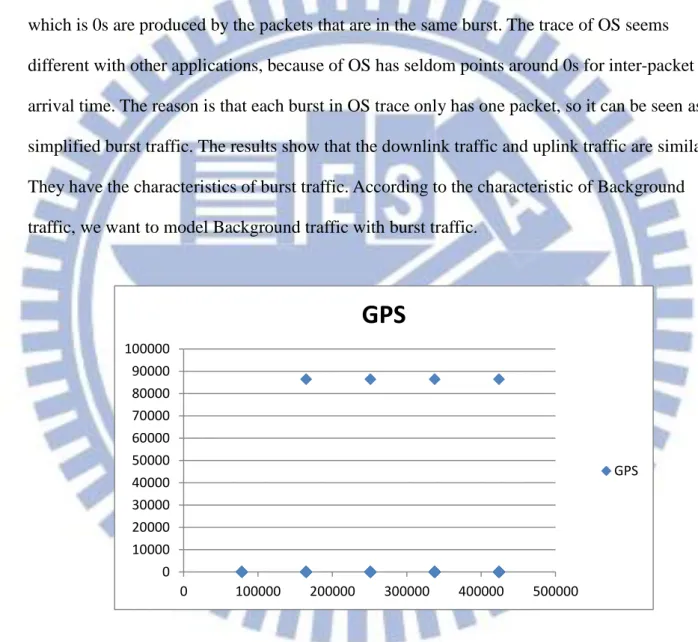
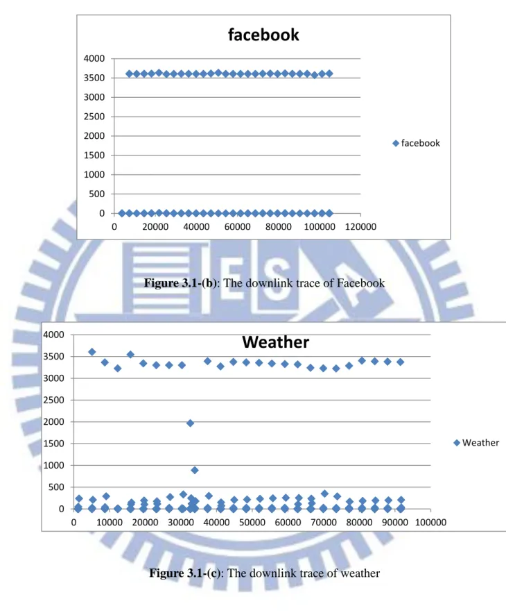
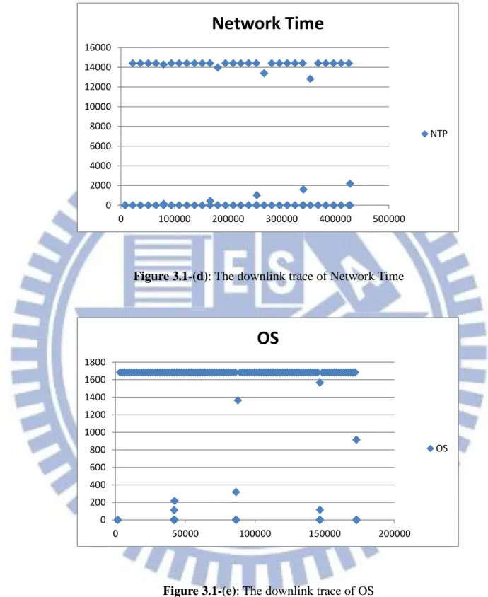
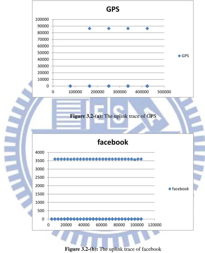
Background traffic is characterized by long periods of inactivity follow by relatively short bursts of activity [12]. This phenomenon shows that the Background traffic for applications updating on mobile device, such as meteorology, stocks, keep alive mechanism, Network time, etc…, are performed as the format of burst traffic and principally with periodic gaps. The trace files we used in this thesis are captured by Shark through Android Phone with different applications. The downlink traces for different applications running in Background mode are shown as Figure 3.1-(a)~(e). The uplink traces for different applications running in Background mode are shown as Figure 3.2-(a)~(e).The packet arrival time for x-axis and inter-packet arrival time for y-axis are shown in the graphs. Each point represents a packet, the graphs show the whole Background traffic of single application (i.e. GPS, facebook, Weather, NTP, OS).
14
The graphs show the characteristics of the Background traffic running with single-application. They nearly have the same characteristic of periodic bursts but with different burst inactivity periods. When the packets are displayed regularly on the axis of inter-packet arrival time with the same value on the graphs means the bursts come
periodically with a specific inactivity period. The points around with inter-packet arrival time which is 0s are produced by the packets that are in the same burst. The trace of OS seems different with other applications, because of OS has seldom points around 0s for inter-packet arrival time. The reason is that each burst in OS trace only has one packet, so it can be seen as simplified burst traffic. The results show that the downlink traffic and uplink traffic are similar. They have the characteristics of burst traffic. According to the characteristic of Background traffic, we want to model Background traffic with burst traffic.
Figure 3.1-(a): The downlink trace of GPS
0 10000 20000 30000 40000 50000 60000 70000 80000 90000 100000 0 100000 200000 300000 400000 500000
GPS
GPS15
Figure 3.1-(b): The downlink trace of Facebook
Figure 3.1-(c): The downlink trace of weather
0 500 1000 1500 2000 2500 3000 3500 4000 0 20000 40000 60000 80000 100000 120000
Weather
Weather16
Figure 3.1-(d): The downlink trace of Network Time
Figure 3.1-(e): The downlink trace of OS
0 2000 4000 6000 8000 10000 12000 14000 16000 0 100000 200000 300000 400000 500000
Network Time
NTP 0 200 400 600 800 1000 1200 1400 1600 1800 0 50000 100000 150000 200000OS
OS17
Figure 3.2-(a): The uplink trace of GPS
Figure 3.2-(b): The uplink trace of facebook
0 10000 20000 30000 40000 50000 60000 70000 80000 90000 100000 0 100000 200000 300000 400000 500000
GPS
GPS 0 500 1000 1500 2000 2500 3000 3500 4000 0 20000 40000 60000 80000 100000 12000018
Figure 3.2-(c): The uplink trace of Weather
Figure 3.2-(d): The uplink trace of NTP
0 500 1000 1500 2000 2500 3000 3500 4000 4500 0 20000 40000 60000 80000 100000
Weather
Weather 0 2000 4000 6000 8000 10000 12000 14000 16000 0 100000 200000 300000 400000 500000NTP
NTP19
Figure 3.2-(e): The uplink trace of OS
Instant Message traffic is more complicated than Background traffic, unlike the periodic characteristic of Background traffic. The traffic may change with different habits of users, so it is difficult to imitate Instant Message traffic with a mathematical traffic model. The information we can obtain from on-line active Instant Message traffic is the average inter-packet arrival time; maximum inter-packet arrival time; minimum inter-packet arrival time; average packet size; average packet count, in a whole Instant Message traffic. The CDFs of the Instant Message traffic Downlink trace is shown in Figure 3.3. The trace files are captured by Shark through Android Phone with different Instant Message applications. It displays the CDFs of different applications may have huge differences about the trace. But it also shows that almost all traces from different applications have the same characteristic of inter-packet arrival time less than 10s. It seems that when the inter-packet arrival time grows to 10s, the CDF approaches to 1. So we can determine that the active Instant Message traffic expires when there are no Instant Message packets captured after 10s from the last Instant Message packet is captured. So the definition of the whole Instant Message traffic is the
0 200 400 600 800 1000 1200 1400 1600 1800 0 50000 100000 150000 200000
OS
OS20
duration from the first Instant Message packet to the packet that without another Instant Message packet is captured in 10s.
Figure 3.3: The CDFs of Instant Message traffic trace
3.2
Burst Traffic
The rough illustration of burst traffic is shown in Figure 3.4. Before defining the burst traffic, we should know the main parameters of burst traffic that can describe it. (1) Inter-burst idle time (2) Burst size (3) Inter-packet arrival time in a burst [13].
10-3 10-2 10-1 100 101 102 103 0 0.1 0.2 0.3 0.4 0.5 0.6 0.7 0.8 0.9 1
Packet Inter-Arrival Time (seconds)
CDF
IM: DL Inter-Arrival Distribution
Skype MSN(eBuddy) MSN(eBuddy)2 FacebookMessenger Whatsapp Whatsapp2
21
(1) Inter-burst idle time: The period between the last packet of a burst and the first packet of the next burst.
(2) Burst size: Number of packets.
(3) Inter-packet arrival time in a burst: The time interval of packets within the same burst.
Figure 3.4: Illustration of burst traffic.
With the three parameters, we can describe burst traffic precisely. To model an on-line traffic into burst traffic, we need a definition for maximum inter-packet arrival time. When inter-packet arrival time is larger than the definition, the packet belongs to the next burst. On the other hand, when inter-packet arrival time is smaller than the definition, the packet belongs to the same burst.
We model the Background traffic of multiple applications with simplified ETSI bursty packet data traffic model. The parameters of simplified bursty packet data traffic distribution are shown in Table3.1. Our purpose is updating the mean value of the three parameters from on-line capturing packets continually, so that we can obtain the information of burst traffic as the characteristic of Background traffic. With a reasonable burst definition, we can obtain the three parameters of simplified bursty packet data traffic distribution, then we can realize the
22
characteristic of Background traffic we are using.
Table 3.1: Parameters of simplified bursty packet data traffic distribution
Parameter distribution mean value
Inter-burst idle time Exponential 1 / 𝜆𝑖𝑏
Number of packets per burst Geometric 𝜇𝑝
Inter-packet arrival time Exponential 1 / 𝜆𝑖𝑝
3.3
System Model
We proposed a mechanism to identify the traffic which is being used. We adopt SVM algorithm to classify on-line packets based on their features. It means we can predict this packet we captured belongs to which label of traffic rapidly because of the SVM algorithm. Then we accumulate these on-line packets and analyze their characteristics with our observation. Sending a message through a mobile device usually generate 2~3 Instant Message packets. We can approximately divide all traffic into active traffic which is actively used from user and Background traffic which is without any user using. There is only one label of traffic (Instant Message traffic) belongs to active traffic being discussed in this thesis. So if we capture more than two Instant Message packets in 10s, we identify that we are in Active mode. If there are less than 2 Instant Message packets captured in 10s, we identify that we are in Background mode.
23
After classifying the label of packets and observing the traffic, we will know which traffic (Background or Instant Message) we are using right away. According to our ideas, we can obtain the parameters of traffic characteristics for Background traffic and Instant Message traffic. If we are in active mode, we can gain average; minimum; maximum inter-packet arrival times, average packet sizes, number of packets in a whole Instant Message traffic based on the observation of inter-arrival time less than 10s. If we are in Background mode, we can gain the mean values of inter-burst idle time, number of packets in a burst, inter-packet arrival time in a burst according to the simulation of bursty traffic packet data distribution. The proposed system model is shown in Figure 3.5.
24
Chapter 4.
Simulation
4.1
SVM Simulation
We want to identify the label of a packet, so we use SVM to classify packets. The trace files are captured by Shark through Android phone. In all simulations, we consider both downlink and uplink traffic. According to the traffic traces, we observed that the traffic using TCP protocol produces ACK packets with 68 bytes packet size. This kind of mechanism in TCP protocol ensures that packets can be sent to the destination. But the ACK packets can’t character the downlink traffic we are using because they are produced to ensure the uplink packets from UE can be sent to the server safely. It is hard to define the ACK packets into any labels of traffic. The ACK packets are bidirectional and might interfere with the downlink traffic we want to character. So we don’t consider ACK packets in this thesis, another reason is ACK packets do not have high priority in delay requirement.
Our training data for SVM includes 5428 Background traffic packets and 2205 Instant Message packets. The packets captured are from GPS, Android, Facebook, Weather, News, NTP, OS, MSN, Whatsapp, LINE. Facebook, MSN, Whatsapp, LINE are the instant message applications.
25
4.1.1
Features Selection
Features to select: (1) packet size; (2) inter-packet arrival time; (3) protocol; (4) source port number; (5) destination port number. The simulation results of features selection are shown in Table 4.1.
Table 4.1: The simulation results of features selection
Features Predicting accuracy of
Background traffic
Predicting accuracy of Instant Message traffic
(1) 90.2 % 62.5 %
(1) + (2) 100 % 0 %
(1) + (3) 97.3 % 68.3 %
(1) + (3) + (4) 100 % 90 %
(1) + (3) + (4) + (5) 100 % 0%
As the simulation results, we select (1).packet size (3) protocol (4) source port number to construct the features space for packet classification. We can reach almost 90% predicting accuracy for both Background traffic and Instant Message traffic. The reason that inter-packet arrival time and destination port number cause the accuracy of Instant Message traffic into 0% is that the values of the two features are random numbers. Because of the number of Background data is larger than the Instant Message data, the predict error may happen when
26
some features are random values that can’t character the traffic.
4.1.2
Accuracy of Prediction
After selecting the combination of features, we can construct a three dimensional feature space from SVM. A packet that is about to be predicted will be put into the feature space with the three values of the features. We change the value of protocol into digital, so that we can capture the value of protocol into a vector. The corresponding values of protocol are shown in Table4.2.
Table 4.2: Protocol and corresponding values
Protocol corresponding value
TCP 1 UDP -1 DNS 2 TLSv1 -2 HTTP 3 ICMP -3 NTP 4 IMF -4 SSL 5
With the training data which includes 5428 Background packets and 2205 Instant Message packets, and the feature space constructed by packet size, protocol, and source port number, we can build a model from SVM algorithm to predict the label of packets.
27
The five testing data trace are collected for five different days and different capturing time. Each trace file has running applications with Android, OS, Weather, NTP, GPS, Amazon, News, Facebook, MSN Whatsapp, LINE. All testing trace includes Background packets and Instant Message packets. After predicting the packets, we get the results and compare with the label that packets belong to. The accuracy of prediction is shown in follows:
Table 4.3-(a): The accuracy of predicting downlink testing data
Testing data Accuracy of prediction Number of data
Trace file 1 100% 160 packets
Trace file 2 100% 43 packets
Trace file 3 94% 69 packets
Trace file 4 96% 1433 packets
Trace file 5 96% 331 packets
Table 4.3-(b): The accuracy of predicting uplink testing data
Testing data Accuracy of prediction Number of data
Trace file 1 100% 343 packets
Trace file 2 100% 71 packets
Trace file 3 100% 244 packets
Trace file 4 98% 2056 packets
28
We can obtain more than 90% predicting accuracy from the training data that we captured and the features we chose. According to the experiment, we found that we can gain higher accuracy of prediction with more training data. The result is shown in Table 4.4. A few Instant Message packets are classified into Background traffic. The reason is that the number of Background data is larger than Instant Message data. So the range that produced by Background traffic vectors are bigger than the range of Instant Message vectors in the feature space. A little prediction error may happen. The way to solve the problem is to capture more Instant Message data. Let the number of Instant Message data approach to Background data.
The advantages of using SVM are the rapid predicting time based on the SVM algorithm and high classifying accuracy based on the features of packets from different types of traffic. The drawback is that when a new traffic type generated, the packets of the traffic may have different features, so SVM probably can’t classify this new type of traffic. If any new traffic type is generated, we should add the data sample into training data sets.
Table 4.4: The accuracy follows by increasing training data
training data predicting accuracy of
Background traffic predicting accuracy of Instant Message 2398 Background packets + 858 IM packets 100% 58% 3171 Background packets + 1345 IM packets 100% 74% 4419 Background packets + 1723 IM packets 100% 84% 5428 Background packets + 2205 IM packets 100% 90%
29
4.2
Burst Simulation
We should have the definition of burst so that we can model it with a bursty traffic. First we should define the burst with a specific value, which is the meaning of maximum inter-packet arrival time within a burst. If the inter-packet arrival time is more than the typical value, this packet belongs to next burst. The metric of burst definition is the ratio of burst count with only 1 packet to burst amount.
4.2.1
Burst Definition
As we mentioned in Section 3.2, the Background traffic is displayed with the form of period burst traffic. The burst idle time changes from 500s to 14400s based on different applications. The meaning of the burst definition is to ensure that the packets should be in the same burst are in the same burst. If the burst definition is too small, then the ratio of burst count with only packet to burst amount becomes higher. If the burst definition is too large, then the ratio becomes lower. As the burst definition becomes larger, the optimum value of the definition is at the moment when the ratio decreased to the low and then it maintained at the same ratio until the burst definition is larger than the burst idle period, then the ratio decreased to 0. We use the traffic displayed in Section 3.2 to simulate. The simulations of ratio of burst count with only one packet to burst amount with different applications are shown as follows:
30
Figure 4.1: ratio of burst count with only one packet to burst amount. The x-axis represents burst definition (second), and y-axis represents the value of ratio.
We can observe that when the burst definition equals to 2s, the ratios of different applications decreased to the low and then maintained at a value until the definitions become larger than the burst idle periods for different applications (500s~14400s). The ratios of some applications are still very high after the burst definition is larger than 2s. The reason is that the original burst only has one packet just like Figure 3-1-(e). The ratio of htc-weather seems very different with other applications. It has two burst idle period with 400s and 3400s then follows by short bursts, so the ratio of htc-weather decreased at the time when the burst definition is 2s, 400s, 3400s. According to our experiments, we can ensure that when we define the maximum inter-packet arrival time within a burst to 2s, the packets belong to the same burst are in the same burst.
31
4.2.2
Bursty Traffic Distribution Parameters
Based on the burst definition of 2s we obtained in Section 4.2.1, we can simulate on-line traffic with bursty traffic distribution. We can identify the Background traffic we are using right away with three parameters in simplified bursty traffic distribution. We have 5 traces of 5 different days running the same applications in Background mode. The following simulation is to examine whether those three parameters that we want to use to represent the traffic are similar under the similar traffic running with same applications in 5 different days. The number of bursts represent the different capturing time in the file. The results are shown in Table 4.5 and Table 4.6.
Table 4.5-(a): The parameters in simplified bursty traffic distribution with 5 different days
running with downlink Background traffic
Mean Inter-packet arrival time (1 / 𝜆𝑖𝑏)
Mean Number of packets per burst (𝜇𝑝)
Mean Inter-burst idle time (1/ 𝜆𝑖𝑝) Number of bursts Day 1 0.159 s 4.3 83.39 s 988 Day 2 0.145 s 4.4 82.89 s 1037 Day 3 0.144 s 4.2 83.73 s 539 Day 4 0.138 s 4.5 82.32 s 158 Day 5 0.160 s 4.6 71.81 s 1186
32
Table 4.5-(b): The parameters in simplified bursty traffic distribution with 5 different days
running with uplink Background traffic
Mean Inter-packet arrival time (1 / 𝜆𝑖𝑏)
Mean Number of packets per burst (𝜇𝑝)
Mean Inter-burst idle time (1/ 𝜆𝑖𝑝) Number of bursts Day 1 0.18 s 4.98 78.23 s 1050 Day 2 0.19 s 5.00 75.70 s 1131 Day 3 0.18 s 4.56 76.90 s 590 Day 4 0.16 s 4.65 74.04 s 181 Day 5 0.18 s 5.21 66.10 s 1284
As the results, the parameters in simplified bursty packet data distribution are similar under the traffic running with same applications in different days and different simulating time. The purpose of the thesis is to identify the characteristics of on-line traffic. If we find the characteristics of traffic change, we can update new DRX parameters according to the characteristics of the new traffic to decrease power consumption. Or when the original DRX parameters sets are not suitable for the traffic we are using, after collecting more information and characteristic of the traffic we can update more appropriate DRX parameters for the traffic. As we saw in Table 4.5 and Table 4.6, the parameters in bursty distribution for day 4 with 181 bursts are similar with day 2 with 1114 bursts. So if a whole traffic with 1114 bursts is produced, we can obtain useful and similar characteristics when we capture only 181 bursts.
33
4.3
Traffic Simulation
Our proposed mechanism is to predict the packet captured from Internet, then examine which mode we are running and calculate the corresponding characteristics of the traffic. If we are at active mode, which means we capture more than two Instant Message packets in the period of 10s, we calculate the average; maximum; minimum inter-packet arrival, average packet size, and number of packet in a whole Instant Message traffic. We continuously update these parameters from on-line packets to represent the characteristics of traffic until the Instant Message traffic expires, which means there are less than 2 Instant Message packets in the period of 10s. If we are at Background mode, we continuously update the parameters of simplified bursty traffic distribution from on line packets until Active mode starts. The original traffic and the results after the traffic identification mechanism we proposed are shown as follows. The x-axis represents packet arrival time; y-axis represents packet size; each point represents a packet.
The result shows that when Instant Message packet comes, the program collects and calculates those parameters every 10 seconds. If there are less than 2 Instant Message packets captured in a period of 10s, the program initializes and resets all parameters. If we are at Background mode and capture a Background packet, the program continuously updates those parameters and displays every 10s. After the simulation, we can automatically identify which traffic mode we are at and obtain the parameters that can identify the traffic characteristics from on-line packets.
34
Figure 4.2-(a): The original Instant Message traffic
35
Figure 4.3-(a): The original Background traffic
36
Table 4.6: The accuracy of predicting 5 testing file with the unit of 10s
Testing data Accuracy of prediction Number of packets
Trace file 1 100% 160 packets
Trace file 2 100% 43 packets
Trace file 3 87.5% 69 packets
Trace file 4 90% 1433 packets
Trace file 5 91% 331 packets
37
Chapter 5.
Conclusion
In this thesis, we address the mechanism of traffic identification to identify the traffic through mobile device in LTE. We propose the packet prediction by SVM algorithm and model the Background traffic with simplified bursty traffic distribution and calculate the parameters to the corresponding traffic type. According to the simulation result, we can briefly obtain the traffic characteristics we are using from the proposed traffic identification mechanism.
38
Bibliography
[1] L. Zhou, H. Xu, H. Tian, Y. Gao, L. Du, L. Chen, “Performance Analysis of Power Saving Mechanism with Adjustable DRX Cycles in 3GPP LTE,” IEEE 68th Vehicular Technology Conference. VTC 2008-Fall, Sept. 2008.
[2] 3GPP, “LTE RAN Enhancements for Diverse Data Applications,” in 3GPP TR 36.822 V0.1.0, 2011-11.
[3] 3GPP “Summary of e-mail discussion [74#33] – LTE: Simulation setup for diverse data applications,” in 3GPP TSG-RAN WG2 #75, Aug 2011.
[4] K. Bennett and C. Campbell,” Support vector machines: Hype or Hallelujah?,” ACM SIGKIDD Explorations, 2(2):1-13, 2000.
[5] H. Kim, K. Claffy, M. Fomenkov, D. Barman, M. Faloutsos, K. Lee, “Internet Traffic Classification Demystified: Myths, Caveats, and Best Practices,” in ACM CoNEXT 2008, December 10-12, 2008.
[6] ETSI, “Universal Mobile Telecommunications System (UMTS); Selection Procedures for the Choice of Radio Transmission Technologies of the UMTS,” Technical Report UMTS 30.03, version 3.2.0, Apr. 1998.
[7] Chandro S. Bontu and E.Illidge, Nortel, “DRX Mechanism for Power Saving in LTE,” in IEEE Communications Magazine, June 2009.
[8] 3GPP, “Analysis on instant message traffic,” in 3GPP TSG-RAN WG2 Meeting #75bis R2-115239, Oct. 2011.
[9] C.W. Hsu, C.C. Chang, C.J. Lin, “A Practical Guide to Support Vector Classification,”
39
[10] Z. Li, R. Yuan, X. Guan, “Accurate Classification of the Internet Traffic Based on the SVM Method,” in IEEE International Communications, 2007. ICC’07.
[11] 3GPP, “Proposed Traffic Scenarios for DDV Evaluation,” in 3GPP TSG-RAN WG2 Meeting #75 R2-114086, Aug. 2011.
[12] 3GPP, “Study of background traffic,” in 3GPP TSG-RAN WG2 Meeting #75bis R2-115178, Oct. 2011.
[13] 3GPP, “Burst Level Analysis of Background and IM Traffic,” in 3GPP TSG-RAN WG2 Meeting #75bis R2-115239, Oct. 2011.