Design and Analysis of a 2-D
Eigenspace-Based Interference Canceller
Cheng-Chou Lee and Ju-Hong Lee,
Member, IEEEAbstract— This paper deals with the problem of
eigenspace-based interference cancellation using a two-dimensional (2-D) rectangular array. An efficient 2-D signal blocking technique is presented to remove the desired signal from the received array data. In conjunction with the 2-D signal blocking technique, a positive definite matrix is further constructed and used to compensate the effect of the signal blocking operation on the sensor noise received by a 2-D eigenspace-based interference canceller (EIC). Therefore, the interference subspace required for computing the optimal weight vector of the designed 2-D EIC can be obtained by simply using conventional eigenvalue decomposition methods instead of any complicated generalized eigenvalue decomposition methods. The performances of the de-signed 2-D EIC under finite samples and steering angle error are also evaluated. The developed theoretical results are confirmed by several simulation examples.
Index Terms—Electromagnetic radiative interference,
interfer-ence concellation.
I. INTRODUCTION
A
DAPTIVE interference cancellation can be used for maximizing the rejection of interference regardless of the interference-to-noise ratio (INR) when processing array data. This goal can be efficiently achieved by utilizing eigenspace-based interference cancellers (EIC’s) as presented in the lit-erature [1]–[6]. A common feature for these EIC’s is that the interference subspace (IS) spanned by the interferers must be first computed. Then, the optimal weight vector is computed by maximizing the output signal-to-noise power ratio (SNR) subject to a constraint of orthogonality to the IS.Notable among these EIC’s is the one presented by [4] due to its several advantages over the others. Using a one-dimensional (1-D) uniformly linear array (ULA) and an ap-propriately designed signal blocking processor which blocks the desired signal from the received array data, it finds the IS through the generalized eigenvalue decomposition (GEVD) of the correlation matrix of the data vector at the output of the signal blocking processor. However, the noise component left in the blocked data vector is no longer spatially white because of using the signal blocking matrix. Hence, finding the required IS for computing the optimal weight vector inevitably resorts to a complicated GEVD. As a result, it is very difficult to evaluate the statistical performance under finite samples and Manuscript received May 20, 1997; revised October 29, 1998. This work was supported by the National Science Council under Grant NSC85-2213-E002-008.
The authors are with the Department of Electrical Engineering, National Taiwan University, Taipei 106, Taiwan.
Publisher Item Identifier S 0018-926X(99)04782-1.
the robust capability against steering angle error for the EIC. Moreover, the technique presented in [4] cannot be extended to process two-dimensional (2-D) array data since its 1-D blocking scheme can not be directly applied to the 2-D case. In the literature, there are practically no papers dealing with eigenspace-based interference cancellation using 2-D adaptive arrays.
In this paper, we present the theoretical results for designing and analyzing an EIC using a 2-D adaptive array. Two 1-D blocking matrices are first designed for both row and column subarrays, respectively. Using the blocked data vectors at the output of these 1-D blocking matrices and the properties of Kronecker product for matrices, a 2-D blocking technique is developed to construct a blocked data correlation matrix that does not contain the desired signal component for computing the IS. However, the noise component in is no longer spatially white, which introduces more complexity in computing the IS. To eliminate this effect, a positive definite matrix is created from the designed blocking scheme and is then added to , where is the background noise power. The resulting data correlation matrix then possesses a noise component which is spatially white. As a result, we can find an orthogonal basis matrix of the IS by performing the conventional EVD and then construct the optimal weight vector using this orthogonal basis matrix. This technique facilitates the analyses of the statistical performance under finite samples and the robust capability against steering angle error for the 2-D EIC. Theoretical results on the expecta-tion of the output signal-to-interference plus noise ratio (SINR) are presented for showing the statistical performance of the 2-D EIC. As to the robust capability against steering angle error, it is shown that the performance of the 2-D EIC may be significantly degraded even if there is a small steering angle error. However, using the proposed 2-D blocking technique with higher order can alleviate the difficulty. The breakdown threshold for the 2-D EIC’s performance due to steering angle error is also derived.
This paper is organized as follows. Section II presents the design of an eigenspace-based interference canceller using a 2-D rectangular array. A 2-D blocking technique is developed and the construction of a positive definite matrix for eliminat-ing the effect of the 2-D blockeliminat-ing operation on the spatially white noise received by the 2-D array is proposed. Section III analyzes the statistical performance under finite snapshots for the designed 2-D EIC. The performance of the designed 2-D EIC in the presence of steering angle error is evaluated in Section IV. Several simulation examples for illustration 0018–926X/99$10.00 1999 IEEE
and confirmation of the theoretical works are provided in Section V. Finally, Section VI gives a conclusion for this paper.
II. DESIGN OF A2-D EIGENSPACE-BASED INTERFERENCE CANCELLER A. The 2-D Array Data Model
Consider a 2-D uniform rectangular array (URA) with sensors located on the - plane at the positions
for and
, where represents the signal wavelength. Let the signal impinging on the array from the elevation angle and azimuth angle yield a unit magnitude response and a phase
response given by at the array
sensor located at , where
and . narrow-band
signals are impinging on the URA from distinct angles
for . Thus, the data received by the
sensor located at can be expressed
as
(1) where denotes the complex waveform of the signal emitted by the th source and the spatially white sensor noise independent of . Without loss of generality, assume that is the desired signal with direction angle
and the other signals are interferers. From (1), the data matrix received by the URA is given by
(2)
where
, and is the received noise matrix. Rewriting (2) in vector form, we have
(3) Using the following property of Kronecker product [7]:
KP.1
where are matrices with appropriate sizes, we can rewrite (3) as
(4) where the response vector of the th signal source
, the response matrix of the signal sources
, and the signal source
vec-tor . The correlation matrix of
is then given by
(5)
where denotes the full rank
corre-lation matrix of the signal sources, the noise power, and
the identity matrix.
B. The 2-D Blocking Technique
In the follwoing, we present a technique for the design of a 2-D EIC with a steering angle . Utilizing the results presented in [4] and letting the steering angle be accordant with the direction angle of the desired signal, we can construct a blocking matrix for the column subarrays of the 2-D URA such that
with and
(6)
where is the order of . is the row
selection matrix which selects the first rows of , where is an zero matrix. Similar results can be obtained for the row subarrays as
with and
(7)
where is the order of . is the row
selection matrix which selects the first rows of . Based on the above results, we present a 2-D blocking technique as follows.
Theorem 1: Let the matrix be given by with and
(8) Then is an autocorrelation matrix of the blocked 2-D array data which contain all the interferers except the desired signal.
Proof: Based on the fact that
, and the property of Kronecker product [7] KP.2
it can be shown that
(9)
where is given by (6) and .
Based on (5) and (9), then we have
(10)
where and
. Based on the fact of and the
property of KP.2, (10) can be further written as
where
, and
. Similar to (11), we have the following result for the row subarrays:
(12)
where . Summing (11) and (12)
yields (13) where (14) and (15) Clearly, is a positive definite matrix if
for all . From (13) to (15), we note that is the autocorrelation matrix of a data vector which does not contain the desired signal component.
C. The 2-D EIC Formulation
Based on the 1-D results of [4], the criterion in finding the optimal weight vector for the 2-D EIC can be defined as maximizing the output SNR subject to a constraint of orthogonality to the IS. Accordingly, we have to solve the following optimization problem:
Maximize subject to range
(16) where serves as the steering vector. The optimal solution of (16) is given by
(17) Equation (17) reveals that the matrix
due to the interferers must be found in order to compute . However, cannot be known a priori. Basically, one can resort to finding a basis matrix spanning range to solve this problem. Unfortunately, the matrix given by (15) is generally not an identity matrix. Hence, we have to perform the GEVD of . Let the generalized eigenvalues and the corresponding eigenvectors be designated as and , respectively. Accordingly, we have the following expression:
(18)
where .
Let , then it can be shown that
range range . Therefore, the optimal weight
vector of (17) can be rewritten as
(19) From (19), we note that performing the complicated GEVD of is inevitable for computing the optimal weight vector .
Moreover, evaluating the statistical performance under finite data samples and the sensitivity to steering angle error for the 2-D EIC becomes very difficult because the GEVD of is necessary for designing the 2-D EIC.
To tackle the above two problems, in Appendix A, an efficient method is presented to construct such a positive definite matrix that the effect of the 2-D blocking operation on the noise component of the received array data can be
eliminated, i.e., . Thus, we obtain
(20) Equation (20) reveals that the corresponding noise component in becomes spatially white. Performing the EVD of , we have the following expression:
(21)
where .
Let the matrix and the matrix
. It is easy to show that and
range range range (22)
i.e., is an orthogonal basis matrix spanning range and is an orthogonal basis matrix spanning the complement of range . It follows from (22) that the optimal weight vector for the 2-D EIC based on the criterion of (16) can be rewritten as
(23) III. STATISTICAL PERFORMANCE
UNDER FINITE DATA SAMPLES
In practice, the number of signal sources , the background noise power , and the ensemble correlation matrix required for implementing the 2-D EIC are not available and usually estimated from the received data snapshots. Using the first data snapshots, we obtain the estimate for the number of signal sources based on the AIC or MDL criterion presented by [11]. Moreover, implementing the AIC or MDL criterion requires performing the EVD of the corresponding data correlation matrix. Therefore, can be estimated by utilizing the eigenvalue method of [12] during the same estimation process. Let the estimated value be denoted as . Then, the next data snapshots are used to compute the sample correlation matrix as follows:
(24)
to replace , where is the data matrix received at the time instant . The correlation matrix of (20) is then replaced by
(25) where
It is appropriate to assume that and are independent in this case. Thus, (21) becomes
(27)
where . Since the number of
interferers is , the corresponding basis matrix of IS
and its complement are given by and
, respectively. Consequently, the optimal weight vector for the 2-D EIC under finite snapshots is given by
(28) The statistical performance of the proposed 2-D EIC under finite data samples is given by the following theorem.
Theorem 2: For the case of input INR high enough, the expectation of the output SINR can be approximately given by
SINR SINR FSP (29)
where SINR denotes the array output SINR without the finite sample effect. FSP represents the factor of statistical performance and is given by
FSP (30)
where
(31) and
(32)
Proof: Please see Appendix B.
If the interferers are uncorrelated, (32) can be further simplified as
(33)
Moreover, we have the following result.
Theorem 3: If the angle separations between the interferers
and the desired signal satisfy that or
for , it can be shown that
SINR SINR (34)
where and are given by (A-11). Proof: Please see Appendix D.
Theorem 3 provides a lower bound of the convergence rate for the proposed 2-D EIC under the situation considered. For example, consider the situation where the direction angle
of the desired signal , the blocking orders
, and the direction angles of interferers
with or for . Then, we
have . A lower bound of the output SINR can be
obtained from (34) and is given by
SINR SINR (35)
Equation (35) shows that a satisfactory convergence speed for the designed 2-D EIC can be guaranteed in this case.
To result in a simpler version of the above theoretical results for providing an insight, we next consider a special situation where all the uncorrelated interferers are located outside the array mainlobe and the angle separations between the desired signal and the interferers are large enough so that
(36) Moreover, and are greater than and , respectively. Based on these two conditions, the optimal weight vector given by (17) can be reduced to an approximation of
and, hence, , the results in (31) can be simplified as the following approximations:
for and for
(37) Then, we can simply substitute (33) and (37) into (30) to obtain the corresponding FSP.
IV. PERFORMANCE ANALYSIS UNDER STEERING ANGLE ERROR
In this case, the steering angle is not accordant with the
direction angle of the desired signal, i.e., .
The blocking factors shown in (6) and (7) become and
(38)
respectively. The mismatch between and
leads to a result that the blocked data correlation matrix given by (8) contains a leakage due to the desired signal and becomes
(39) where
, and , respectively. Since
for all is a positive definite matrix.
which are greater than and the corresponding eigen-vectors spans the subspace range . The computed basis matrix will contain more than principal eigenvectors of if the number of interferers is overestimated. From (23), the optimal weight vector corresponding to this case is given by
(40) This leads to the result that the 2-D EIC fails to work due
to that range contains the vector and the
constraint of .
Next, consider the situation where the number of interferers is exactly known and the desired signal is uncorrelated with the interferers. Based on (39), we have
(41)
where denotes the power of
the desired signal leakage in the output after the 2-D blocking
operation. , where is given by (14) except
that the entries of and are now given by (38). Let the nonzero eigenvalues and the corresponding eigenvectors
of be given by and for
, respectively. For further simplicity, assume that the interferers are located far away from the desired
signal so that for .
Then, the eigenvalues which are greater than and the corresponding eigenvectors of can be approximated as
and for
and , respectively.
Note that consists of the first principal eigenvectors of . As a result, consists of for
when . Hence, range range
and the 2-D EIC works normally. On the other hand,
contains the normalized response vector if
. From the optimal weight vector given by (40), we note that the desired signal will be suppressed due to the constraint of . As shown by (38) and the fact that is proportional to , this difficulty could be alleviated by increasing the orders and if the steering angle error is small. In general, the breakdown threshold happens when is nearly rank-deficient.
To look into the effect of , we proceed to
consider the case of two uncorrelated and closely separated interferers.
Let the two uncorrelated interferers be closely separated so
that . From [8, pp. 25–27], we
can easily show that
(42)
where for and .
and are given by
Hence, the condition causing the performance
failure becomes
(43)
When and are small enough, it is also
shown in [8] that
(44)
Substituting (44) into (43) and taking the first-order approxi-mation yields the following performance breakdown threshold
(45)
V. COMPUTER SIMULATION EXAMPLES
In this section, several simulation examples for illustrating and confirming the theoretical works are presented. The 2-D array used for all simulations is a URA with and . Moreover, the simulation results based on the direct GEVD of given by (18) to obtain an IS basis matrix required for computing the optimal weight vector are also presented for comparison.
Example 1: This example is performed to illustrate the theoretical results presented in Section III. We set
. The desired signal with input dB is impinging
on the array from . One interferer has input
dB. The first data snapshots are used
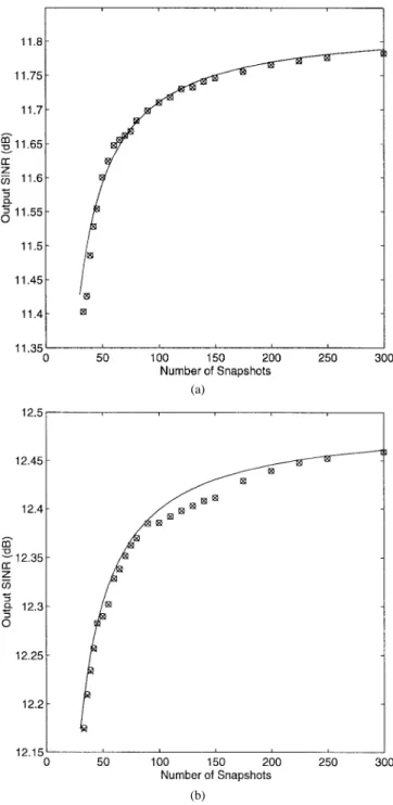
to estimate the source number and the noise power . Fig. 1 plots the array output SINR in dB versus the number of snapshots for two different interfering angles. Each simulation result is obtained by averaging 100 independent runs with independent noise samples for each run. The solid curve represents the theoretical results computed by using (29) based on (28) and (30)–(32). This confirms the validity of (29) given by Theorem 2. On the other hand, the curve with “x” represents the simulation results for the performance of the 2-D EIC designed by using the proposed technique, while the curve with “o” represents the simulation results of the 2-D EIC designed by using the direct GEV2-D technique. The coincidence between these two curves shows that the 2-D EIC designed by using the proposed technique provides the same performance as that directly using the complicated GEVD technique.
Comparing the results of Fig. 1(a) and (b), we note that the output SINR of Fig. 1(a) is smaller than that of Fig. 1(b) for each number of snapshots as expected because the angle separation between the desired signal and the interferer is smaller for Fig. 1(a). This phenomenon is further demonstrated in Fig. 2 by plotting the FSP of (30) versus the interfer-ing angle . We note that FSP increases and hence the performance degradation increases as approaches
(a)
(b)
Fig. 1. The results of Example 1. Output SINR versus the number of snapshots for the case of one interferer. Solid line: The theoretical result. “x”: The 2-D EIC using the proposed technique. “o”: The 2-D EIC using the direct GEVD technique. (a)(u2; v2) = (0:11; 0:13). (b) (u2; v2) = (0:14; 0:12).
Example 2: This example considers the case of multiple interferers. Again, we set . The desired signal
Fig. 2. The factor of statistical performance (FSP) versus the interfering angle for Example 1.
with input dB is impinging on the array from
, while the uncorrelated interferers have the
same input dB. The first data snapshots
are used to estimate the source number and the noise power . Fig. 3 depicts the array output SINR in decibels versus the number of snapshots for different interfering situations. Each simulation result is obtained by averaging 100 independent runs with independent noise samples for each run. The solid curve represents the theoretical results computed by using (29) based on (28) and (30)–(32). In contrast, the dash curve represents the theoretical results computed by using (29) based on the approximations described by (37). The dash curve almost coincides with the solid curve. This confirms the validity of the approximations given by (37). Moreover, the coincidence between the curves with “x” and “o” illustrates that the 2-D EIC’s designed by using the proposed technique and directly using the complicated GEVD technique have the same performance.
Example 3: Here, we illustrate the performance of the designed 2-D EIC in the presence of steering angle error.
The steering angle is . The desired signal
with input dB is impinging on the 2-D array
from . Two uncorrelated interferers
with input dB are impinging on the array from
and . To
evaluate the sensitivity to the angle separation , we define a robustness index (RI) as follows in (46), shown at the bottom of the page, for the designed 2-D EIC and (47), shown at the bottom of the page, for the 2-D EIC directly
RI
The output SINR using of (40)
The output SINR using of (17) with replaced by
(46)
RI The output SINR using of (19) with replaced by
The output SINR using of (17) with replaced by
(a)
(b)
Fig. 3. The results of Example 2. Output SINR versus the number of snap-shots. Solid line and dash line: The theoretical results. “x”: The 2-D EIC using the proposed technique. “o”: The 2-D EIC using the direct GEVD technique. (a) Two interferers with(u2; v2) = (0; 0:6) and (u3; v3) = (0:55; 0:45). (b) Three interferers with(u2; v2) = (0; 0:6), (u3; v3) = (0:55; 0:45) and (u4; v4) = (0:5; 0).
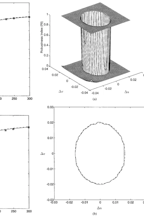
using the complicated GEVD technique. Fig. 4(a) plots the RI versus . The top curve represents the RI versus , while the bottom curve represents the RI versus . It shows that the proposed technique possesses the advantage of robust capability against steering angle error over the GEVD technique. Fig. 4(b) depicts the curves of the breakdown threshold for RI . The dash curve represents the breakdown threshold computed by (45), while the solid curve represents the simulation results. This figure also confirms the presented theoretical results.
(a)
(b)
Fig. 4. The performance comparison for Example 3. (a) Robustness index versus the interfering angle separation(1u; 1v). The top curve: The 2-D EIC using the proposed technique. The bottom curve: The 2-D EIC using the direct GEVD technique. (b) The breakdown threshold curves of the 2-D EIC using the proposed technique. Solid curve: The simulation results. Dash curve: The theoretical results.
VI. CONCLUSION
The theoretical works for the design and analysis of a 2-D eigenspace-based interference canceller (EIC) have been pre-sented. An effective 2-D signal blocking technique is first presented to remove the desired signal from the received array data. To compensate the effect of the signal blocking operation on the sensor noise, a positive definite matrix has been constructed. Therefore, the interference subspace required for computing the optimal weight vector can be obtained by using conventional eigenvalue decomposition methods. The performances of the designed 2-D EIC under finite samples
and steering angle error have been evaluated, respectively. The developed theoretical results are confirmed by several simulation examples. It has been shown that the performance of the designed 2-D EIC is the same as that of a 2-D EIC directly using a complicated GEVD technique in the situation without steering angle error. However, the proposed 2-D EIC possesses the advantage of more robust capability against steering angle error over the 2-D EIC based on the GEVD technique.
APPENDIX A
Let be an cyclic-shifting matrix defined as (A.1)
where is the th column vector of the identity
matrix. Following the results presented in [4], the blocking matrix which satisfies (6) can be constructed as follows:
(A.2)
where is an vector given by
(A.3) and are the coefficients satisfying
(A.4) The subscript “ ” denotes the complex conjugate. From (A.2)
and (A.3), it can be seen that is an Hermitian
and Toeplitz matrix. Furthermore, let HT
denote an Hermitian and Toeplitz matrix with its first
row given by . Then, we have
HT
with (A.5)
Next, we construct an vector as follows:
(A.6)
where and is an integer. From (A.6),
an matrix is constructed as follows:
(A.7) Using (A.6) and (A.7), we have
HT (A.8)
From (A.8), we note that is positive definite, Hermi-tian, and Toeplitz. Moreover, it is easy to show that
HT
(A.9)
for , where and denote
the real and imaginary parts of , respectively.
if , and , otherwise. We then construct a positive definite matrix as follows:
(A.10) Summing (A.5) and (A.10) thus yields a diagonal matrix as follows:
(A.11) where denotes the proportional constant. Following the same procedure, we can find a positive definite matrix
such that for some positive . Finally,
we form the following matrix:
(A.12) Based on (15) and the property of Kronecker product [7]
KP.3
for matrices and with appropriate sizes, we can easily
show that , where .
APPENDIX B
Here, we show the result given by (29) in Theorem 2. Per-forming the EVD of , we obtain the following expression: (B.1)
where and
. Similarly, we have the fol-lowing expression:
(B.2) from the EVD of , where
and . From (20) and (25),
the deviation between and due to finite sample effect can be expressed as
(B.3)
where and . Using (8) and (26),
is given by
(B.4) Following the first-order perturbation analysis presented in [9], we can show that
(B.5) where
It follows from (B-6) that possesses the following prop-erties:
and (B.7) Substituting (B.5) into (28) and preserving only the first-order term, we obtain the following approximation for the optimal weight vector under finite samples:
(B.8) Using (B-8) and the property that , we can find the powers of the desired signal, the noise, and the interferers at the array output as follows:
the first-order terms
the first-order terms the first-order terms
(B.9)
where , and
represent the output powers of the desired signal, the noise, and the interferers without finite sample
effect, respectively. denotes the input power
of the desired signal. is negligible when the 2-D EIC works normally. The other terms are the second-order perturbation terms which are given by
(B.10)
(B.11) and
(B.12) respectively. Since is negligible, the output SINR of the 2-D EIC can be written as
SINR
(B.13) Consider the situation where the number of data snapshots is large enough. Utilizing the first-order approximation of for a small , we can obtain an approximation for (B-13) as follows:
SINR SINR
(B.14)
where SINR represents the output SINR without
finite sample effect. Since the expectation for each of the first-order terms in (B-9) is zero, the expectation of the output SINR can be approximated from (B-14) as follows:
SINR SINR
(B.15)
where and .
Next, we compute the individual terms in (B.15). As shown in (B.3), the deviation is composed of two independent terms, i.e., and . By using the eigenvalue method of [12] to estimate the noise power, it has been shown that
(B.16) if data snapshots are used. On the other hand, it has been shown in [10] that the deviation due to finite sample effect has zero mean and the second-order statistical property as
(B.17) where are matrices with appropriate sizes. By substituting (B.5) into (B.10)–(B.12) and using the properties of (B.7), (B.16), and (B-17), the individual terms in (B.15) are com-puted. The results are listed in Appendix C. It is also shown
in Appendix C that the term LE is dominant in
the case of input INR high enough since all the other terms decrease as the input INR increases. Accordingly, (B-15) can be approximately expressed as
SINR SINR FSP (B.18)
for input INR high enough, where the factor of statistical
performance FSP LE is given by (30).
APPENDIX C
To ease the presentation, we employ the subscripts and to replace the subscripts “ ” and “ ”, respectively. For
example, and represent the notations and ,
respectively. Thus, (B-4) can be rewritten as
(C.1) Using the above notations and performing some algebraic manipulation provides
(C.3)
(C.4)
(C.5) and
(C.6)
respectively, where and
(C.7)
for , respectively.
Next, let the positive definite matrix be expressed as for some positive number and positive definite matrix . Then it can be easily shown from (B.7) that is
proportional to . From (C.2) to (C.7), it can also be shown that each of the following terms:
and (C.8)
is proportional to and each of the following terms:
and
(C.9)
is proportional to , while only the term is
fixed and independent of . To get a further simplification, consider the case that is large enough, i.e., the input INR is high enough so that these terms in (C.8) and (C.9) are
negligible as compared to . Then, we have the
result as shown by (B-18).
APPENDIX D
By using the Cauchy–Schwarz inequality that
(D.1) where and are matrices with appropriate sizes, it follows from (31) and (32) that
(D.2) Based on (30) and (D.2), it can be shown that
FSP (D.3)
Substituting (31) into (D.3), we obtain FSP
(D.4)
where denotes the maximal eigenvalue of .
Fur-thermore, based on (A.11) and the property of Kronecker product [7]
KP.4
where denotes the determinant of the matrix , it can be shown that
(D.5) Therefore, we have
FSP (D.6)
If the interferers are uncorrelated, (33) reveals that both
and are not greater than . Thus,
the inequality in (D.6) becomes
From (6), it can be shown that if .
Similarly, we have if . Thus, if
or , we have
for . Hence, (D.7) reduces to
FSP (D.8)
Finally, substituting (D.8) into (29) yields the result shown by (34).
REFERENCES
[1] M. G. Amin, “Concurrent nulling and locations of multiple interference in adaptive antenna arrays,” IEEE Trans. Signal Processing, vol. 40, pp. 2658–2663, Nov. 1992.
[2] H. Subbaram and K. Abend, “Interference suppression via orthogonal projections: A performance analysis,” IEEE Trans. Antennas Propagat., vol. 41, pp. 1187–1193, Sept. 1993.
[3] B. Friedlander, “A signal subspace method for adaptive interference cancellation,” IEEE Trans. Acoust., Speech, Signal Processing, vol. 36, pp. 1835–1845, Dec. 1988.
[4] A. M. Haimovich and Y. Bar-Ness, “An eigenanalysis interference canceler,” IEEE Trans. Signal Processing, vol. 39, pp. 76–84, Jan. 1991. [5] Y. Bressler, V. U. Reddy, and T. Kailath, “Optimum beamforming for coherent signals and interference,” IEEE Trans. Acoust., Speech, Signal
Processing, vol. 36, pp. 833–842, June 1988.
[6] K. Ohnishi and R. T. Milton, “A new optimization technique for adaptive antenna arrays,” IEEE Trans. Antennas Propagat., vol. 41, pp. 525–532, May 1993.
[7] A. Graham, Kronecker Products and Matrix Calculus with Applications. New York: Ellis Horwood, 1981.
[8] J. E. Hudson, Adaptive Array Principles. New York: Peter Peregrinus, 1981.
[9] F. Li and R. J. Vaccaro, “Unified analysis for DOA estimation algorithms in array signal processing,” Signal Processing,vol. 25, pp. 147–169, Nov. 1991.
[10] M. Kaveh and A. J. Barabell, “The statistical performance of the MUSIC and minimum-norm algorithms in resolving plane waves in noise,” IEEE
Trans. Acoust., Speech, Signal Processing, vol. ASSP-34, pp. 331–341,
Apr. 1986.
[11] M. Wax and T. Kailath, “Detection of signals by information theoretic criteria,” IEEE Trans. Acoust., Speech, Signal Processing, vol. ASSP-33, pp. 387–392, Apr. 1985.
[12] P. Stoica, “On estimating the noise power in array processing,” Signal
Processing, vol. 26, pp. 205–220, Feb. 1992.
Cheng-Chou Lee was born in Taipei, Taiwan, on July 20, 1969. He received the B.S. and Ph.D. degrees in electrical engineering from the National Taiwan University, Taipei, Taiwan, in 1991 and 1997, respectively.
His current research interests include the adap-tive signal processing, array signal processing, and the signal processing in wireless communication systems.
Ju-Hong Lee (S’81–M’83) was born in I-Lan, Taiwan, on December 7, 1952. He received the B.S. degree from the National Cheng-Kung University, Tainan, Taiwan, in 1975, the M.S. degree from the National Taiwan University, Taipei, Taiwan, in 1977, and the Ph.D. Degree from Rensselaer Polytechnic Institute, Troy, NY, in 1984, all in electrical engineering.
From September 1980 to July 1984, he was a Research Assistant and was involved in research on multidimensional recursive digital filtering in the Department of Electrical, Computer, and Systems Engineering at Rensselaer Polytechnic Institute. From August 1984 to July 1986, he was a Visiting Associate Professor and later in August 1986 became an Associate Professor in the Department of Electrical Engineering, National Taiwan University. Since August 1989, he has been a Professor at the same university. He was appointed Visiting Professor in the Department of Computer Science and Electrical Engineering, University of Maryland, Baltimore, during a sabbatical leave in 1996. His current research interests include multidimensional digital signal processing, image processing, detection and estimation theory, analysis and processing of joint vibration signals for the diagnosis of cartilage pathology, and adaptive signal processing and its applications in communications.
Dr. Lee received Outstanding Research Awards from the National Science Council in the academic years of 1988, 1989, and 1991–1994.