First-order analysis of a three-lens zoom system with the last lens fixed

This article was downloaded by: [National Chiao Tung University 國立交通大學] On: 28 April 2014, At: 05:12

Publisher: Taylor & Francis

Informa Ltd Registered in England and Wales Registered Number: 1072954 Registered office: Mortimer House, 37-41 Mortimer Street, London W1T 3JH, UK

Journal of Modern Optics

Publication details, including instructions for authors and subscription information:

http://www.tandfonline.com/loi/tmop20

First-order analysis of a three-lens zoom

system with the last lens fixed

Mau-Shiun Yeh a , Shin-Gwo Shiue b & Mao-Hong Lu b a

Chung Shan Institute of Science and Technology , PO Box 90008-8-10, Lung-Tan, Tao-Yuan, 325, Taiwan

b

National Chiao Tung University, Institute of Electro-Optical Engineering , 1001 Ta Hsueh Road, Hsin Chu, 30050, Taiwan Published online: 03 Jul 2009.

To cite this article: Mau-Shiun Yeh , Shin-Gwo Shiue & Mao-Hong Lu (1998) First-order analysis of a three-lens zoom system with the last lens fixed, Journal of Modern Optics, 45:2, 363-375, DOI: 10.1080/09500349808231695

To link to this article: http://dx.doi.org/10.1080/09500349808231695

PLEASE SCROLL DOWN FOR ARTICLE

Taylor & Francis makes every effort to ensure the accuracy of all the information (the “Content”) contained in the publications on our platform. However, Taylor & Francis, our agents, and our licensors make no representations or warranties whatsoever as to the accuracy, completeness, or suitability for any purpose of the Content. Any opinions and views expressed in this publication are the opinions and views of the authors, and are not the views of or endorsed by Taylor & Francis. The accuracy of the Content should not be relied upon and should be independently verified with primary sources of information. Taylor and Francis shall not be liable for any losses, actions, claims, proceedings, demands, costs, expenses, damages, and other liabilities whatsoever or howsoever caused arising directly or indirectly in connection with, in relation to or arising out of the use of the Content.

This article may be used for research, teaching, and private study purposes. Any substantial or systematic reproduction, redistribution, reselling, loan, sub-licensing, systematic supply, or distribution in any form to anyone is expressly forbidden. Terms & Conditions of access and use can be found at http://www.tandfonline.com/page/terms-and-conditions

JOL'RK.41, O F X10I)ERN OPI'ICS, 1998, VOL. 45, NO. 2, 363-375

First-order analysis of a three-lens zoom system with the

last lens fixed

M A U - S H I U N YEH

Chung Shan Institute of Science and Technology, PO Box 90008-8-10, Lung-Tan, Tao-Yuan 325, Taiwan

S H I N - G W O S H I U E and M A O - H O N G LU

National Chiao T u n g University, Institute of Electro-Optical Engineering, 1001 T a Hsueh Road, Hsin C h u 30050, Taiwan

(Received 18 March 1997; revision received 3 July 1997)

Abstract. A general analysis for the first-order solutions of three-lens zoom system with the last lens fixed is presented. The reasonable solution areas in the focal length diagrams are derived and shown graphically. The relation between the separation of the two front lenses and the image distance of middle lens in zooming is found to be a hyperbola. According to the different locations of centre of hyperbola, four cases are analysed. From the four hyperbolic graphs, we get six different types of zoom system. For each zoom type, we find the maximum range of focal length and the position where the maximum or minimum system length occurs during zooming.

1. Introduction

A zoom system is generally considered to consist of three parts: the focusing, zooming and fixed parts. T h e focusing part is placed in front of t h e zooming part, to adjust the object distance. T h e zooming part is literally used for zooming and the fixed rear part serves for controlling the focal length or magnification and reducing the aberrations of the whole system. Several of the published papers [1-4] concerning zoom have concentrated on the first-order zoom design. A two-optical- component method for designing zoom system has been proposed [2] and a three- lens zoom system with one lens fixed has been solved by this method. T h e three- lens system with the last lens fixed is widely used in many zooming systems, such as cameras, but the solution area has not been analysed so far.

In this paper, we use the grapho-analytical method [5] to solve the first-order layout of a three-lens zoom system with the last lens fixed. T h e possible solution areas in the focal length diagram are shown graphically. W e find the relation between the separation of the two front lenses and the image distance of middle lens in zooming, which can be described by a hyperbola. W e obtain four hyperbolae corresponding to the different positions of centre of the hyperbola. From the four hyperbolic graphs, we can get six types of zoom system and find the maximum variation range of focal length for each zoom type. T h e zoom position where the system has the maximum or minimum length is discussed.

0950-0340/98 $12.00 0 1998 Taylor & Francis Ltd.

3 64 M . - S . Yeh et al. u,=o a H H’ 0 5

l---d1--l--dz+l~+

*-D2+

Figure 1 . Gaussian diagram of three-lens zoom system with the third lens fixed. S(S’) is the distance from the first (second) lens to the first (second) principal plane H(H’) in the combined unit.

2. Theory 2.1. Basic formulae

In figure 1, an infinite-conjugate three-lens zoom system, with the last lens fixed and the others moving, has been analysed by the two-optical-component method [2], in which lenses 1 and

2

are combined as the first component and the last lens is regarded as the second component. T h e combined component has the focal length Fl2 and power K12. dl and d2 are the interlens separations between lenses 1 and 2 and between lenses 2 and 3 respectively.

6’

is the distance from the second lens to the second principal plane H’ in the combined unit. K and F are the equivalent power and focal length respectively of the system. T h e related equa- tions are then given by

1; = (1 - M3)F3,

where 1; and M3 are the image distance and magnification of the F3 lens. Solving the above equations, from equations (1)-(4), we have

d2 =

-(&-

1)F3

+

( 1 - g ) F 1 2 . (7) Because the third lens is fixed during zooming, M3 is constant. F is therefore proportional to Fl2. In zooming, we change F and then obtain Fl2, dl and d2.

From paraxial optics, we have

First-order analysis of three-lens zoom system

Comparing equation (7) with equation (S), we find that

Substituting equation (6) into equation (9), we have

1; = (1 -$)F2.

365

(8)

2 . 2 . Solution areas in the focal length diagram

T h e interlens separations dl and d2 must be positive in zooming. T h i s gives

some constraints on the solutions, that is on F l , F2 and F3. Because the third lens is fixed, the image point of F2 is also fixed during zooming. I n this case, we can always find a lens F3 to form a final real image from the lens equation and have a positive d2, no matter where the image point of F2 is. So we shall discuss only the solution areas under the constraint of positive dl

.

F r o m equation (6), we have

F I

+

F2 - - F 1 F 2 2 0. Fl2

According to the different signs of Fl2, we have two cases as follows:

and

T h e curve for (Fl - Fl2)(F2 - Fl2) - F:, = 0 is a hyperbola with its centre at

(F12, F12) in the FI-F2 coordinate graph. T h e solution distribution in the graph is thus divided into several areas by the hyperbolic curves. Each solution area has different solution ranges for Fl2 and d l .

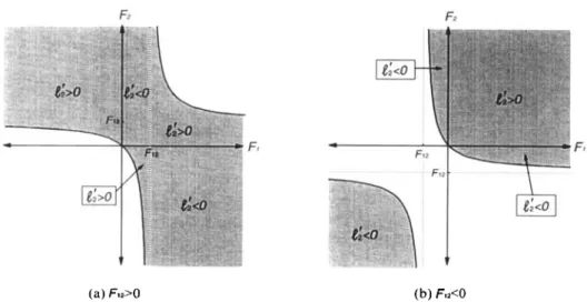
From the above analysis, we can illustrate the possible solution areas in the focal length diagrams according to the different combinations of Fl and F2, and the sign of F12. Figure 2 shows the solution areas for Fl2

>

0 and Fl2

<

0 under t h e condition of positive d l . T h e power signs of Fl and F2 in each area are shown in parentheses as ( F l , F2). T h e sign of F I

+

F2 is positive in the upper right section and negative in the lower left section. T h e solution ranges of Fl2 and d l , and the

related range o f 1; obtained from equation (10) for each solution area are shown in tables 1 and 2 with different signs of Fl2. Using equation (lo), we can show the sign of 1; for each solution area in figure 3.

2.3. Relation between the separation dl and the image distance of

I;

From equations (3) and (9), we have

[dl - ( F I

+

F2)](l; - F2) - F i = 0

or

Table 1. Solution ranges of F12, dl and 1; for different solution areas under different combinations of lens types with positive F 1 2 .

w Possible location of

vertex of related lenses Solution area Range of F I 2 Range o f dl Range o f 1; Used segment hyperbolic curve Types of

-m < 1;

<

- F I F ~ Segment 2a Positive transverse 0

<

dl < F1

+

F2 Fl

+

F2 (01 > 0 , a2 > 0 ) axis(dl

>

0 , 1; = 0 )

<

Fl2 < Fl > 0 , F2

>

0 ( I ) in figure 2(a) (++) Fl

+

F2 FI F2 F 1 + F 2 < d l < O O F 2 < 1 ; < 0 0 Segment Ib

F,

<

0 , F2

>

0 (IIa) in figure 2(a) 0 < F12 < 00

Quadrant I

(-+) ( 4 > 0 , a2 > 0 )

Segment 3

( 0 1

<

0, 0 2 > 0 ) Quadrant I, I1

(IIb) in figure 2 ( a ) FiF2 0

<

dl

<

00 Fl F2

0

<

FI2

<

- F2 < 1;

<

-

Fl

+

F2 F I

+

F2

Fl

<

0, F2

<

0 No solution No solution No solution No solution No solution No solution (---)

(+-)

FI

>

0 , F2

<

0 (IVa) in figure 2(a) 0 < F12 < 00 F l + F , < d l < 0 0 F 2 < 1 ; < 0 0 Segment 5 Positive transverse

is

(01

>

0 , a2

<

0 ) axis(dl > 0, I; = 0 )

(IVb) in figure 2(a) FlF2 O<dl < 00

O < F l 2 < - FI

+

F2

Fl F2 Segment 4a Positive transverse ‘c

axis(dl > 0 , I; = 0 ) _$

F2 < 1;

<

-

Fl

+

F2 (ai < 0, a2

<

0 )

4 E Table 2. Solution ranges of F12, dl and 1; for different solution areas under different combinations of lens types with positive F I 2 .

Possible location of vertex of related Range of FI2 Range o f dl Range of 1; Used segment hyperbolic curve Types of

Fl

>

0 , F2

>

0

lenses Solution area

(I) in figure 2(b) -00

<

F I 2

<

0 F l + F 2 < d 1 < 0 0 F2<1;<00 Segment 1 a

Quadrant I

(++) (a1 > 0, 0 2

>

0 )

Fl < 0, F2 > 0 (11) in figure 2(b) FI F2 0

<

d1 < Fl

+

F2 Fl F2 Segment 2b Negative transverse

--OO < Fl2

<

-

(-+) Fl

+

F2 -m<1;<- Fl

+

F2 (a1

>

0 , a2

>

0 ) axis(dl

<

0 , 1; = 0)

Fl

<

0, F2

<

0 (111) in figure 2(b) F l F 2

_<

O < d I < O 0 Fl F2 Segment 4b Negative transverse

F12 < 0 F2

<

1;

<

-

(--I

Fl

+

F2 Fl

+

F2 ( 4

<

0 , a2 < 0 ) axis(dl

<

0, 1; = 0 ) Quadrant 111. IV FI > 0 , F2

<

0 ( I V ) in figure 2(b) FlF2 O G d l < F l + F 2 - m < l ; < Fl F2 Segment 6 -00 < FI2

<

-

(+-I

Fl

+

F2 Fl

+

F2 (ai > 0, a2

<

0 )

First-order analysis of three-lens zoom system 367

( a ) F+O (b) Ft2<0

Figure 2. Solution areas (shaded) for different combinations of lens types under the condition of positive d l : ( a ) Fl2 > 0; ( b ) Fl2 < 0.

( a ) F+O (b) Fu<O

Figure 3 . Sign distributions of 1; in the solution areas: ( a ) Fl2

>

0; ( b ) Flz < 0.

where a1 = Fl

+

F2 and a2 = F2

T h e above equation describes a hyperbola with its centre at the coordinates ( a , , a2) in the dl -1; coordinate graph. Because the centre of the hyperbola can be

located in one of the four quadrants depending on the signs of al and a2, we obtain

four cases of hyperbolae shown in figures +7. T h e upper right hyperbolic curve

has the vertex Vl with dl = a1

+

IF21 and 1; = a ; !

+

IF21 and the lower left

hyperbolic curve has the vertex V2 with dl = a1 - IF21 an 1; = a2 - 1F21. Because

a2 = F z , one of the hyperbolic curves always intersects the transverse ( d l ) axis at

one vertex of hyperbola, that is Vl or Vz. I n figure 4, Fl could be positive o r

negative. I f F1

>

0 (or F1

<

0) is selected, the vertex V2 is located on the positive transverse (or negative) axis. A similar situation occurs in figure 6.

368 M . 3 . Yeh et al. t:

e:

di=FjiFi at pointy:

e:

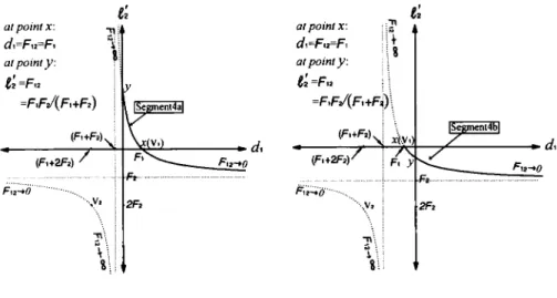
=F,? =FF~/(F~+F*) atpointx: atpointy:

(b) a+0, a00, and F60 Figure 4. Hyperbola with its centre in the first quadrant of the d1-1; coordinate

diagram. V1 and V2 are the vertices of the hyperbola. T h e intersection coordinates of hyperbola and two axes are x and y respectively: ( a ) F1

>

0; ( b ) F1 < 0.

a60 and &>O

Figure 5 . Hyperbola with its centre in the second quadrant of the dl-1; coordinate diagram.

From e q u a t i o n s (6) and (lo), w e c a n solve the focal length Fl2 f o r each point on t h e h y p e r b o l a as follows:

or

First-order analysis of three-lens zoom system 369

e:

Y' di=Fiz=F, "1 8 at point x at poinr y

(a) c?1<0, &<O, and Fi>O (b) ~ 6 0 , ~ 6 0 , and F60 Figure 6. Hyperbola with its centre in the third quadrant of the dl-1; coordinate

diagram. ( a ) Fl > 0; ( b ) F1

<

0.

e:

at point x' atpoinry: dt=Fte=Fi

e;

= F ~ ~ =F~FJ(F~+F~)

u+O and UZ<O

Figure 7. Hyperbola with its centre in the fourth quadrant of the dl-1; coordinate diagram.

In equation (16), if dl approaches infinity, Fl2 approaches zero. Similarly, if 1s in

equation (17) approaches infinity, Fl2 approaches infinity and the sign of F12 is determined by the sign of -(Fl/F2)1;. T w o cases for different signs of F l / F 2 are obtained. If F I / F ~

<

0, the values of Fl2 for the points on the upper-right and lower left hyperbolic curves are positive and negative respectively. O n the other hand, if F , / F 2

>

0, the values of Fl2 for the points o n the upper right and lower left hyperbolic curves are negative and positive respectively.

In figure 4-7, the intersections of the hyperbola and the two axes are x and y corresponding to 1; = 0 and d , = 0 respectively. As described before, x is t h e vertex V l o r V 2 . T h e value of Fl2 can be obtained from equation (17) by 1; = 0. S o we have

370 M . 3 . Yeh et al.

Substituting equation (18) into equation (6), we get

dl = F I .

Similarly, the values of Fl2 and 1; at y obtained by d1 = 0 in equations (16) and (17). We have

As mentioned before, a reasonable separation dl must be positive in zooming.

So only the segments of hyperbola in the right-hand half of the dl-1; coordinate graph are acceptable and shown as solid curves in figures 4-7. Six segments are found and labelled Segment followed b y a number. Each segment represents the characteristics of a zoom system, including the constraints on al and a2 (or on Fl

and F2) and the solution ranges of F12, dl and 1; in zooming. Therefore we can have six types of zoom system. In figures 4 and 6, the segment labels are followed by an extra letter a or b for two different combinations of F1 and F2.

T h e length of zoom system, which is the distance from lens 1 to image plane, is the sum of d l , l ; , -13 and 1;. T h e last two terms are constants because the third lens

is fixed. From the property of a hyperbola, the value of d1

+

1; has a minimum at the vertex Vl with dl = al

+

IF21 and 1; = a2

+

IF21 for segments 1 , 3, 4 and 5 and has a maximum at the vertex V2 with dl = a1 - IF21 and 1; = a2 - IF21 for segments

2 and 6. So the system length has an extreme value (maximum or minimum) at some position of zooming, that is not necessarily at one end of zooming, if the vertex of the hyperbolic curve is located in the right-hand half of the dl-1;

coordinate graph. In this case, the value of Flz is calculated as follows.

Substituting dl = al

+

IF21 or 1; = a2

+

IF21 into equation (16) or (17) for segments 1, 3, 4 and 5 , we have

{

;:

i f F 2

>

0, if F2

<

0. F12 =

Similarly, substituting DI = a1 - IF21 or 1; = a2 - IF21 into equation (16) or (17) for segments 2 and 6, we have

if F2

>

0,

{

-?I ifF2 < 0 . Fl2 =

On the other hand, if the vertex of hyperbolic curve falls in the left-hand half of the

dl-1; coordinate graph, the maximum and minimum system lengths occur at the

two ends of zooming.

2.4. Related segment of hyperbola f o r different solution areas

In section 2.2, we have analysed the reasonable solution areas in the focal length diagrams and their related solution ranges of Fl2, dl and 1;. From sections

2 . 2 and 2.3, we find that the ranges of Fl2, dl and 1; for each solution area shown in

figure 2 and listed in tables 1 and 2 are always a part of hyperbola in one of the four

First-order analysis of three-lens zoom system 371 1 " " ' " " " " ' " 1 10

-

8 -

2

6 ; h

2 .

s

4 -

2

- . 0 2 - k 0 - 8 7 6 5 4 3 2 1

Distance to image plane

Loci of three-lens zoom system with F1 = -1, Fz = 1.2, F3 = -0.5, M3 = 2 and a zoom ratio of 2 5 : l . T h e dotted line indicates the image position of middle lens. T h i s system has dl = 1 4 , 1; = 2.4 and Fll = 1 at the position where the system length is minimum during zooming.

Figure 8.

cases in figures 4-7, where dl is positive. T h e sixth and seventh columns in tables 1

and 2 show the constraints on the signs of al and a2, the used segment of hyperbola, and the possible vertex locations of related hyperbolic curve in the four quadrants for each solution area. T h e various quadrants are denoted ( I ) , (11), ( I I I ) and ( I V ) respectively.

2.5. Six types of zoom systems

Figures 4-7 have shown that each of the six segments represents the char- acteristics of a zoom system. Six different types of zoom system are thus discussed as follows.

2.5.1. Type I

For segment 1 in figure 4, the range of F12 starts from plus or minus infinity t o zero depending on the sign of F l / F 2 . From tables 1 and 2, we find that two solution areas with positive F2 meet this type. Because the vertex of related hyperbolic curve falls in the first quadrant of the dl-1; coordinate graph, the system length always passes through a minimum value during zooming. In this type, we choose the second solution area in table 1 as an example. According to the constraints on Fl and F2 in the solution area (IIa) in figure 2 ( a ) , we have Fl = -1 and Fl = 1.2. Referring to the solution range of l i , we have F3 = -0.5 and M3 = 2 to keep d2 positive during zooming. I n theory, Fl2 can be from plus infinity to zero. here we choose the range of F12 from 5 to 0.2 with a zoom ratio of 2 5 : l . T h e focal length range of system is from 10 to 0.4 given b y equation (4). When the system length has the minimum value, we have dl = 1.4, 1; = 2.4 and Fl2 = 1. T h e lens loci in zooming are shown in figure 8, with the focal length F as ordinate. the image position of the middle lens, that is the object position of the third lens, is fixed and shown as a dotted line.

2.5.2. Type I I

For segment 2 in figure 4, the range of Fl2 is from plus or minus infinity t o

F I F ~ / ( F I

+

F2). In tables 1 and 2, two solution areas with positive F2 belong to

372 0 4 h ’

fs

0 3 - M . 5

4

0 2 -

v

-

0 1 - 0 M . - S . Yeh et al. L -

;

:

lens1 lens

this type. the vertex of the related hyperbolic curve is located on the transverse axis. If the vertex is on the positive transverse axis, the system has a maximum length in zooming with dl = F l , 1; = 0 and Fl2 = F l . Here we choose the second solution area in table 2 as an example. According to the constraints on F1 and F2 in the solution area (I I) in figure 2 ( b ) and the range of l i , we have Fl = - 1, F2 = 10,

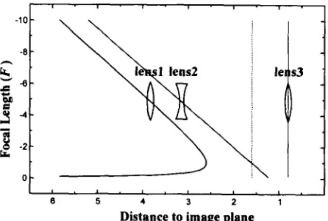
F3 = 4 and M3 = -0.05. We have the theoretical range of Fl2 from minus infinity to -1.111. In this example, we choose Fl2 from -9 to -1.5 with a zoom ratio of 6 : 1. T h e zoom loci are shown in figure 9.

2.5.3.

T y p e 111

For segment 3 in figure 5, the range of Fl2 is from FlF?/(FlF2) to 0. Only the third solution area in table 1, with positive F12 and F2, belongs to this type. In this case, the vertex of related hyperbolic curve can be located in the first or second quadrant. With the constraints on F1 and F2 in the solution area ( I I b ) in figure 2 ( a ) and the range of

Li,

we have F1 = -1, F2 = 0.95, F3 = -2 and

M3 = 1.5. In theory, the maximum range of F12 is from 19 to 0. In this example, we choose F12 from 4 to 0.25. T h e system has a zoom ratio of 16:l and has the minimum length with dl = 0.9,li = 1.9, and F12 = 1. T h e zoom loci are shown in figure 10.

2.5.4.

Type

IV

For segment 4 in figure 6, the range of Fl2 is from F ~ F ~ / ( F I

+

F2) to 0. In tables 1 and 2, two solution areas with negative F2 belong to this type. I n this case, the vertex of the hyperbolic curve is located on the transverse axis. Here we use the sixth solution area in table 1 as an example. Using the solution area (IVb) in figure 2(a) and the range of l;, we have Fl = 1, F2 = -1.2, F3 = 2 and M3 = -1. We have the theoretical range of Fl2 from 6 to 0. I n this example, we choose F12 from 1.5 to 0.1. T h e system has a zoom ratio of 15:l and has the minimum length with

dl = 1, 14 = 0 and F12 = 1. T h e zoom loci are shown in figure 11.

First-order analysis of three-lens zoom system 373

I " " " " " I

o

5 3 2 1

l

Distance to image plane

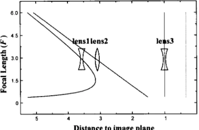
Figure 10. Loci of three-lens zoom system with F1 = -1, F2 = 0.95, F3 = -2,

M 3 = 1.5, 1; = 1 and a zoom ratio of 1 6 : l . This system has dl = 0.9, 1; =, 1.9 and

Fll = 1 a t the position where the system length is minimum during zooming.

0 0

1

20 18 16 14 12 10 8 6 4 2

Distance to image plane

Figure 11. Loci of three-lens zoom system with F I = 1 , Fz = -1.2, F R = 2, M3 = -1,

I ; = 1 and a zoom ratio of 15:l. This system has dl = 1 , l;,= 0 and Flz = 1 at the position where the system length is minimum during zooming.

2.5.5. T y p e V

F o r segment 5 in figure 7, the range of Fl2 is f r o m plus infinity to zero. O n l y the tifth solution area in table 1 belongs t o this type. T h e vertex of hyperbolic curve is located on the positive transverse axis. By using t h e solution area (IVa) in figure 2 ( a ) a n d the range of l i , we have Fl = 1 , F2 = -0.4, F4 = 0.4 a n d 1 C I 3 = -1. In this example, we choose the range of Fl2 from 1 0 to 0.1 with a zoom ratio of 10O:l. T h e system has t h e m i n i m u m length with dl = 1, 1; = 0 a n d Fl2 = 1. T h e zoom loci are shown in figure 12.

2.5.6. Type VZ

F o r segment 6 in figure 7, the range of Fl2 is f r o m m i n u s infinity to

F I F z / ( F I

+

F2). Only t h e fourth solution area in table 2 with negative F2 a n d

F12 belongs to this type. T h e vertex of hyperbolic curve can b e located in t h e third or fourth quadrant. Referring to t h e solution area (IV) in figure 2 ( h ) a n d t h e range

374 M.-S. Yeh et al.

position where the system length is minimum during zooming. I 2.5

-

h 4 2.0 -

3

.

v A '

21.5-

-

cr.

8

lo: 0 5 - 1.5 1 .o 0.5

Distance to image plane

0

Figure 1 3 . Loci of three-lens zoom system with F1 = 1, F2 = -0.2, F3 = 0.4, M3 = -1, 1; = 0.8 and a zoom ratio of 1 O : l . T h i s system has d , = 0.6, 1; = -0.4 and F12 = -1 at the position where the system length is minimum during zooming.

of l i , we have F1 = 1, F2 = -0.2, F3 = 0.4 and M3 = - 1 . In this example, we choose the range of Fj2 from -2.5 to -0.25 with a zoom ratio of l O : l , We get

Fl2 = 1; = -0.25 at dl = 0. T h e system has the minimum length with dl = 0.6, 1; = -0.4 and F12 = - 1. T h e zoom loci are shown in figure 13.

3. Conclusion

For designing a zoom system, the size of system and the slope of lens loci have been taken into account. From figures 8-13, we find that the lens locus of the middle lens is linear. This is due to the linear relationship between Fj2 and 1; in equation (10). In some types, we may have an interlens separation of zero at one end of zooming. Usually, it is not useful to work in the neighbourhood of the end in a practical design. I n this paper, we have not discussed the special condition in which a1 = 0 (F1

+

F2 = 0). I n this case, the solution is easily obtained by the

First-order analysis of three-lens zoom system 375 same way as described in section 2. T h e centre of the hyperbola in equation (1 5 ) is located on the longitudinal axis in the dl-1; coordinate graph.

In this paper, we have analysed the possible solutions areas in the focal length diagrams, the relation between dl and l;, and the properties of lens loci during zooming. With the help of the solution range of l i , the values of F3 and M3 are

easily obtained to get a final real image and to keep d2 positive in zooming. T h e

analyses of six system types, corresponding to six segments in the d1-l; coordinate

graph, are very helpful for designers to select the positive and negative types of three lenses, to preview the shape of lens loci and to determine the ranges of F12, dl and 1;.

Acknowledgment

China under grant No. NSC-85-2215-E-009-004.

This project was supported by the National Science Council of the Republic of

References

[ l ] M.wN, A , , and THO~IPSON, B. J. (editors), 1993, Selected Papers on Zoom Lenses, SPIE [2] YI:II, M. S., S H I U E , S. G., and Lu, M. H., 1995, Opt. Engng, 34, 1826.

[3] Y E I I , M. S., SHIUE, S. G., and L L ~ , M. H., 1996, Opt. Engng, 35, 3348. [ 4 ] YI’H, M. S., S I I I U E , S. G., and Lu, M. H., 1997, Opt. Engng, 36, 1249. [5] O s t i o ~ s t i ~ ’ , M. L . , 1992, Opt. Engng, 3 1 , 1093.

Milestone Series, Vol. MS 85 (Bellingham, Washington: SPIE).