Dynamics and thermal instability of magnetic flux in type-II superconductors

Dynamics and thermal instability of magnetic flux in type-II superconductors

B. Ya. Shapiro,1,_{*I. Shapiro,}1_{B. Rosenstein,}2_{and F. Bass}1 1_{Department of Physics, Bar Ilan University, Ramat Gan 52100, Israel}

2_{Department of Electrophysics, National Chiao Tung University, Hsinchu, Taiwan, Republic of China.} 共Received 8 June 2004; revised manuscript received 17 November 2004; published 17 May 2005兲 In recent experiments, trapped magnetic flux is initially generated by abrupt laser heating of a strip of a type-II superconducting film subjected to a weak magnetic field. We study herein the nonequilibrium penetra-tion of the flux into the Meissner state area. Effects of the heat dissipapenetra-tion and transport on the mopenetra-tion and stability of the interface between the magnetic flux and flux-free domains are considered. It is shown that the magnetic induction and the temperature have the form of a shock wave moving with constant velocity as large as that corresponding to the depairing current. In the vicinity of the front, superconductivity is suppressed by strong screening currents. The front velocity is determined by the Joule heat caused by the electric current in the normal domain at the flux front. The stability of the shock wave solution is investigated both analytically and numerically. For sufficiently small heat diffusion constant a finger shaped thermal instability is found.

DOI: 10.1103/PhysRevB.71.184508 PACS number共s兲: 74.20.De, 74.25.Ha, 74.25.Qt

I. INTRODUCTION

The dynamics of magnetic flux penetration into a type-II superconductor and its instabilities have been studied by a variety of techniques over the years,共see Ref. 1, and refer-ences therein兲. Magneto-optics experiments2 _demonstrate that in a wide range of situations there exists a well-defined interface 共front兲 between the magnetic flux penetrating into the sample and the flux-free Meissner state. Improvements to these magneto-optical techniques have revealed a wide class of instabilities, including magnetic macroturbulence3,4_{and a} dendritic instability.5_{The instability of the magnetic flux and} flux avalanches are observed both in anisotropic high tem-perature superconductor4 and in an isotropic material like Nb.5

Traditionally there are three possible scenarios in which the instabilities could arise. The standard thermomagnetic instabilities appear when the critical vortex state6 _is per-turbed locally by the heat released by a moving vortex. This dissipation leads to the thermal softening of the vortex sys-tem which in turn is responsible for the instability.1 _{In this} case the instability develops around a well defined thermo-dynamically stable Bean state. There is no moving front in this case. A different type of thermal instability, namely the thermal overheating instability of the steady flux-antiflux front, was considered theoretically by some of us.7 _{In this} case the excess heat released at the front is caused by vortex-antivortex annihilation. Yet another type of instability occurs in strongly anisotropic superconductors.8,9 _{In this case the} stationary vortex-antivortex interface is destroyed by the Thomas-Kelvin instability.

Recently, a type of flux instability was observed experi-mentally. In these experiments superconductivity was locally destroyed in a completely nonadiabatic fashion by a femto-second laser pulse.10_{The pulse clearly forces the system out} of thermal equilibrium. The superconductivity is destroyed inside a narrow strip of a YBCO film subjected to a magnetic field perpendicular to the film. The field does not exceed the first critical field Hc1, so that initially fluxons cannot

pen-etrate the rest of the sample. Therefore the magnetic flux

initially fills the normal domain. Recovery of superconduc-tivity occurs in two stages. Once the short pulse is over, the strip cools and the flux nucleates into a dense system of Abrikosov vortices. The characteristic time of that stage is microscopic, of order of the Ginzburg-Landau 共GL兲 relax-ation time共appearing in the time dependent GL equations兲

t_GL⬃10−10_{s. This process has been studied by us some time} ago11 _{and we do not address this stage in the present paper} since it was shown that no instability is originated at this stage.

On the larger共mesoscopic兲 time scale the rapidly created vortices are pushed into the superconducting part of the sample. The fluxons move very fast with velocities of order of 105 cm/ s 共in YBCO兲.10 The flux flow currents, J, in this case are much higher than the critical current Jctypical for

the thermodynamic Bean model critical state, but smaller

共although not much smaller兲 than the depairing current Jd:

J_d⬎JⰇJ_c. Just after the vortex nucleation stage the mag-netic flux forms a rapidly moving front. This highly nonequi-librium relaxation dynamics is very different from the essen-tially adiabatic dynamics of the critical state discussed earlier. The front line shape is not always stable: sometimes it dynamically develops dendriticlike structures.12

The existence of the sharp and typically straight front can be in principle understood in the framework of the theory of nonlinear magnetic flux diffusion.13,14 _{Geshkenbein et al.} considered the flux diffusion in the creep regime, while Sha-piro et al.14 considered the flux flow regime. In both cases the temperature gradient effects were neglected and no insta-bility of the front was predicted, namely, it was shown that corrugation of the front line is unfavorable. The front veloc-ity under these assumptions decreases with time.14_However, corrugation of the front is typically caused by thermal effects,1_{hence, one expects that in the case of fast dynamics} of the front, these effects are even more important.

In the present paper we study both numerically and ana-lytically the dynamics of the nonadiabatically created mag-netic flux in sufficiently thick共thickness larger than the mag-netic penetration length兲 superconducting films. In particular, effects of dissipation and the heat transport on the motion

and stability of the flux front are considered. It is shown that the Joule heat released at the flux front can produce front propagation at constant velocity inside the type-II supercon-ductor. Heating of the front by the moving magnetic flux is essential. We found that for certain voltage–current charac-teristics of the superconductor in its resistive state, the mag-netic induction penetrating a flux-free superconductor forms a sharp front. Strong superconducting currents in the vicinity of the front suppress superconductivity in this area and create a normal domain at the front. The interface moves with

con-stant velocity which is completely determined by the Joule

heat released in the normal domain at the leading edge of the front. The straight front line shows an instability with respect to local temperature fluctuations. In fact an excessive local temperature at the front leads to excessive Joule heat re-leased there and in turn increases the local front velocity in the area of the fluctuation. The hydrodynamical tangential instability of the flux front destroys the flat front. Numerical simulation of the exact set of nonlinear equations allows us to study the evolution of the instability and demonstrates the emergence and development of the corrugated interface.

II. MODEL AND BASIC EQUATIONS A. Hydrodynamics of the vortex matter

(for the slab geometry)

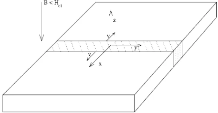
Let us consider a typical experimental situation共see Ref. 12兲, when a relatively thick 共with thickness larger than mag-netic penetration depth ␭兲 type-II superconducting film is subjected to a weak external magnetic field 共B⬍Bc1兲. The

magnetic induction B therefore has only a z component Bz

⬅B and all dependencies on the z coordinate can be

ne-glected. The two dimensional vortex systems is described by the magnetic induction B共r,t兲 and the temperature profile

T共r,t兲, where r=共x,y兲 is a two dimensional vector. To derive

the hydrodynamic equations one starts from the continuity equation for the fluxon density n共r,t兲=兺a␦关r−ra共t兲兴 and the

flux current I_i共r,t兲=兺_av_ia共t兲␦关r−ra共t兲兴. Here i=x,y and a

= 1 ,…N labels the fluxons. The continuity equation

⳵n

⳵t = −ⵜiIi 共1兲

supplemented by the constituent relation

Ii共r,t兲 = Df共r,t兲ⵜin共r,t兲 共2兲

leads to the flux diffusion equation ⳵n共r,t兲

⳵t = −ⵜi关Df共r,t兲ⵜin共r,t兲兴. 共3兲

Since n共r,t兲=B共r,t兲/␾0, where␾0is the unit flux, the Max-well equation

−1

c

⳵B

⳵t =␧ijⵜiEj 共4兲

leads to the identification Ei=共c/␾0兲␧ijDf共r,t兲ⵜjn共r,t兲,

while␧ijis the antisymmetric tensor. Since in the mixed state

of the type-II superconductor E = RJ, where R共B,T兲 is the

resistivity, one obtains R =共4␲/␾₀2兲Df. The electric current

density in turn is equal to Ji=共c/4␲兲␧ijⵜjB. The flux

diffu-sion equation then takes the form 4␲ c2 ⳵B ⳵t = ⳵ ⳵x

冋

R ⳵B ⳵x

册

+ ⳵ ⳵y

冋

R ⳵B ⳵y

册

. 共5兲

The function R共B,T兲 will be phenomenologically defined in the next subsection. In the normal state the same equation applies with the normal state resistivity.

Now we turn to the heat transport equation, identical to the conventional normal state heat balance equation

C⳵T

⳵t = Dⵜ

2_{T + J · E共B,T兲 −␥C共T − T}

0兲. 共6兲 Here C is the heat capacity and D is the heat diffusion con-stant, T0 is the temperature of the cooling liquid with ␥ = 1 / tr being the heat relaxation constant, when tr the heat

relaxation time. The first term on the right hand side is the heat conduction, the second is the Joule heat, and the third describes the heat exchange between the slab and the cooling liquid. The Joule heat term consists of two different contri-butions. In the mixed state it is dominated by the motion of the magnetic flux, while in the normal metal when the super-conductivity is suppressed by the currents, one has usual Ohmic resistance losses.

In the geometry we consider共see Fig. 3兲, the dependence of both the temperature and the magnetic induction on z can be neglected. The magnetic induction is independent of z, since thickness of the thick film 共slab兲 in the z direction is assumed to be larger than the magnetic penetration length␭, while the temperature is uniform in the z direction, despite the presence of the last term, since the thermal diffusion length is typically much larger than the film’s thickness. The detailed argumentation is presented in Ref. 15.

B. Resistivity at high currents

As a rule, the nonlinear resistivity R共J,B,T兲 ⬅E共J,B,T兲/J in the mixed state of a type-II superconductor

is a complicated function of magnetic field, current and tem-perature, see Fig. 1. In this work we will be interested mainly in resistivity at currents much larger than the critical current

Jc, when the pinned vortices are released. The vortex

resis-tivity grows quickly above Jc either exponentially or as a

power R⬀J␮with large ␮. In this relatively low current re-gime the dependence of the resistivity on magnetic induction

B is very smooth 共roughly linear兲. However, when the

cur-rent approaches the depairing curcur-rent Jd the power ␮

be-comes smaller and resistivity strongly depends on B. Recently detailed measurements of the I–V characteristics of Nb films at high current density of order 106_{A / cm}2_were performed.16Near the depairing current it has the form

R共B,T兲 = Rn共T兲

冋

J Jd共T,B兲

册

␮

. 共7兲

Here R_n共T兲 is the normal state resistivity. The dependence of the depairing current J_d on magnetic field and temperature16 can be fitted well by the following form:

Jd共T,B兲 = Jd0⌬

冋

Bc2共T兲

B

册

␯/␮

. 共8兲

The upper critical field depends on temperature as B_c2共T兲 = B_c2共0兲⌬, where we assumed that dimensionless tempera-ture␪= T / Tcis not far from 1, namely⌬⬅1−␪ is small.

When the current exceeds Jd共B,T兲, the electric field is

continuous, the resistivity saturates at its’ normal value

R共B,T兲=Rn共T兲. The derivative of R appearing in the

nonlin-ear flux diffusion Eq.共5兲 is discontinuous. We fitted the I–V curves of Nb and obtained␮= 1.5 with temperature indepen-dent Rn. For Nb at fields of the order of Bc1 we obtain the

best fit␯= 1.3. The values of other material parameters are:

Bc2共0兲=4.43 T, Rn= 9.9␮⍀ cm and Tc= 8.6 K. These were

measured directly. The obtain the best fit for the constant

Jd0= 9.2· 106A / cm2. See Fig. 2 for a sample of data taken at

T = 7.8 K,␪= 0.9.

Of course the exponents depend on material and weakly depend on field for larger magnetic fields. The power law however generally holds. Examples include YBCO well

above Bc1 共see Ref. 17兲 in which the power law is clearly

seen, but ␮= 2, ␯= 2. The corresponding data on high Tc

superconductors are not yet available for fields below B_c1, to our knowledge, and therefore we treat the powers as phe-nomenological parameters 共see also Refs. 14 and 18兲. An additional difference between the conventional and the high

Tcmaterials is that the normal state conductivity in high Tc

cuprates is linear共“strange metal”兲.

C. Boundary and initial conditions

In a typical experiment12_{the heat of the laser beam} sup-presses superconductivity in a narrow strip of width l divid-ing the sample into two equal superconductdivid-ing parts of length Lxon both sides of the irradiated strip. Magnetic flux

promptly fills the normal area and forms a nonequilibrium vortex strip state. Subsequently the laser is switched off and sample is cooled 共see Fig. 3兲. The set of Eqs. 共5兲 and 共6兲 must be supplemented by the initial and boundary conditions in the center of the sample and on the sample’s edges. The initial temperature is assumed to be homogeneous

T共x,y,t = 0兲 = T0, 共9兲

where T₀ is the temperature of the cooling liquid. Magnetic field fills the irradiated area of width l and magnetic flux of magnitude

⌽ = 2lLyB0=

冕

B共x,y,t兲dxdy 共10兲 is assumed to be trapped in superconductor and conserved. Here L_yis width of the sample. The boundary conditions for temperature are

T共x = ± Lx,y = ± Ly,t兲 = T0. 共11兲 An alternative boundary condition for the magnetic induction which we consider independently is fixed magnetic field at the center B共x=0兲=B0, while B共x= ±Lx兲=0.

FIG. 1. Schematic plot of the nonlinear resistivity of a type-II superconductor in the mixed state as a function of current. The resistivity is zero below the critical current J_c, exponentially small in the flux creep regime just above Jc and evolves into a power function in the flux flow regime. At the depairing current it merges with the Ohmic normal state resistivity.

FIG. 2. A fit of the resistivity dependence on the current density of Ref. 16 to the model resistivity Eqs.共7兲,共8兲 with exponents ␯ = 1.3,␮=1.5. Magnetic field is 20 mT 共circles兲, 30 mT 共stars兲 and 40 mT共squares兲.

FIG. 3. The geometry of the problem. The dashed area contains the flux that penetrated the sample during the initial period in which superconductivity was destroyed in a narrow strip around x = 0. The arrows marked withv indicate the direction of the flux front

mo-tion. The direction of the magnetic field B is perpendicular to the xy plane.

D. Basic equations in terms of dimensionless quantities Dimensionless coordinate, time, and magnetic induction are defined using natural units of length x*= cRn共T=Tc兲

⬅cRn, magnetic field B*=

冑

4␲CTcand time

t*= 4␲R_n

冉

4␲RnJd0 B*

冊

␮

冋

Bc2共0兲 B*

册

␯ 共12兲 as follows: x→ x/x*; t→ t/t*; b = B/B*. 共13兲 For the free electron gas B* _is

B*⬇ Hc1

␭2_k

FvF

c␰ , 共14兲

where ␭, kF, vF, and ␰ are the London penetration length,

Fermi momentum, Fermi velocity, and the coherence length respectively.

Using the scaled variables, the set of nonlinear coupled equations in the superconducting state关J⬍Jd共B,T兲兴 reads

⳵b ⳵t = ⳵ ⳵x

冉

␳ ⳵b ⳵x

冊

+ ⳵ ⳵y

冉

␳ ⳵b ⳵y

冊

, 共15兲 ⳵␪ ⳵t =␬ⵜ 2_␪+␳j2_{−⌫共␪−␪} 0兲, 共16兲

where the dimensionless resistivity and the electric current density are ␳=Rn共␪兲 Rn

冉

b ⌬

冊

␯

冉

j ⌬

冊

␮ ; j =

冑

冉

⳵b ⳵x

冊

2 +

冉

⳵b ⳵y

冊

2 共17兲

and␪0= T0/ Tc. The unit of current density is cB*/ 4␲x*. The

flux diffusion equation does not contain parameters, while the heat transfer equation has two: the dimensionless tem-perature diffusion constant␬and the relaxation coefficient⌫:

␬= Dt *

Cx*2, ⌫ =␥t

*_{. 共18兲}

In the region in which superconductivity is suppressed by the superconducting current J exceeding the depairing cur-rent value Jd共B,T兲, the normal state resistivity becomes R

= Rn共T兲. In this case the basic equations are

⳵b ⳵t = ⳵ ⳵x

冉

␳n ⳵b ⳵x

冊

+ ⳵ ⳵y

冉

␳n ⳵b ⳵y

冊

, 共19兲 ⳵␪ ⳵t =␬ⵜ 2_␪+␳ nj2−⌫共␪−␪0兲, 共20兲 where the dimensionless normal state resistance is defined by

␳n共␪兲 = Rn共␪兲

c2t*

4␲x*2. 共21兲

In the following section we solve these equations both ana-lytically and numerically.

III. STRAIGHT FLUX FRONT FOR␮=0 A. Asymptotics in the superconducting phase

When the boundary conditions are independent of y 共see notations in Fig. 3兲, the front is straight and the problem becomes one dimensional. We start with a case when the resistivity depends only on magnetic induction. Hence, now we consider␮= 0, returning to the general case in Sec. IV A. In addition we initially solve a simplified set dropping the relaxation term ⌫=0 and diffusion ␬= 0. This assumption will be supported a posteriori by calculating the terms’ ef-fects and comparing with the numerical solution.

Looking for a solution of Eqs.共15兲 and 共16兲 in the form

b = bs共X兲, ⌬ = ⌬s共X兲, 共22兲

where X = x − Vt is the distance from the interface and V is the interface velocity, one obtains

− Vdbs dX = d dX

冋

冉

bs ⌬s

冊

␯_db s dX

册

, 共23兲 Vd⌬s dX = PJ. 共24兲

Here the Joule power density is PJ=␳j2. Let us first

investi-gate the asymptotics of bs共X兲 in the vicinity of the front X

→0. In the cold superconductor, the magnetic field vanishes.

Therefore formally 共ignoring formation of the very narrow normal region near the front which will be discussed in the next subsection兲 we look at the magnetic field bs共X兲 as a

power with coefficient dependent on velocity only for X

⬍0:

bs共X兲 = A共V兲兩X兩␣. 共25兲

The temperature is assumed to be of the form

⌬s共X兲 = ⌬s0−⌬s1共V兲兩X兩␤. 共26兲

Substituting the Ansatz Eqs.共25兲 and 共26兲 into Eqs. 共23兲 and

共24兲, one obtains on the superconducting side of the front 共X⬍0兲:

VA␣兩X兩␣−1= A␯+1⌬_s0−␯␣关共␯+ 1兲␣− 1兴兩X兩共␯+1兲␣−2, 共27兲

A2+␯␣兩X兩2␣−2+␣␯=⌬s1␤⌬s0␯V兩X兩␤−1, 共28兲

which is satisfied for

␣= 1/␯; ␤= 2/␯; 共29兲 A共V兲 = ⌬s0共␯V兲1/␯; ⌬s1共V兲 = 1 2⌬s0 2_共 ␯V兲2/␯. 共30兲 The electric current j =⳵bs/⳵X formally diverges as

兩X兩1/␯−1 _{at the front for ␯⬎1. Of course the divergence is} intercepted by the phase transition into the normal state cre-ating the “hot” region of presumably small width wn

deter-mined by the condition that the depairing current is reached

j共X = − w_n兲 = j_d=⌬_s0V共␯Vw_n兲1/␯−1_{. 共31兲} There is also dissipation in the superconducting part of a larger width w_s. The expression for the Joule heat term

caused by the magnetic flux motion everywhere, not neces-sarily close to the front interface, diverges at the front as关see Eq. 共25兲兴 PJ⬀兩X兩2/␯−1 for ␯⬎2 only. Its integral, however,

always converges.

To determine V , wn, and other characteristics of the front

motion we need the solution in the normal domain. This and its matching with the asymptotics in the superconductor is considered next.

B. Solution in normal domain for the temperature independent resistivity

In the normal domain we assume first we assume for sim-plicity that ␳n共T兲=const in addition to the previously used

simplification␬=⌫=0. The nonlinear wave Ansatz

b = b_n共X兲, ⌬ = ⌬_n共X兲 共32兲

will be initially used to find the current density jn

=共db_n/ dX兲. Substitution of Eq. 共32兲 into the normal state Eqs.共19兲 and 共20兲 leads to the following set in terms of the front variable X = x − Vt: − Vjn=␳n djn dX, 共33兲 Vd⌬n dX =␳njn 2_{. 共34兲}

The first equation has a solution

jn共X兲 = jn0exp

冋

− XV ␳n

册

⬇ jn0

冉

1 − XV ␳n

冊

. 共35兲

The approximate form is generally valid since 共兩X兩V/␳n兲

⬍共wnV /␳n兲Ⰶ1 as will be justified a posteriori. Then the

heat transfer equation and the boundary condition⌬n共X=0兲

=⌬0gives ⌬n共X兲 = ⌬0− ␳njn0 2 2V2

再

exp

冋

− 2XV ␳n

册

− 1

冎

⬇ ⌬0+ j_n02 V X. 共36兲

In this region most of the heat is released

⌶n⬅

冕

−w_n 0 ␳n共␪兲

冉

⳵bn ⳵X

冊

2 dX⬇␳njn 2 wn. 共37兲

We will use this result later.

C. Matching solutions on the superconductor-normal interface and the flux front velocity

The current, temperature, and the temperature gradient are all continuous on the superconductor-normal interface lo-cated at X = −w_n. Consequently the current on the normal side approaches the same depairing current as that on the super-conducting side, see Eq. 共31兲. The temperature matching conditions are ⌬共− wn兲 = ⌬0− j_d2wn V =⌬s0, 共38兲 ⌬

⬘

共− wn兲 = j_d2 V= ⌬s0 2 ␯w_n共␯Vwn兲 2/␯_{. 共39兲}

The only solution of the set of three algebraic Eqs.共31兲,

共38兲, and 共39兲 is very simple V = jd 2⌬0 关1 +

冑

1 + 4⌬₀/␯兴 ⬇ jd ⌬0

冉

1 +⌬0 ␯

冊

, 共40兲 wn⬇ ⌬0 ␯jd , 共41兲 ⌬s0⬇ ⌬0− ⌬0 2 ␯ . 共42兲

The front velocity is determined by the Joule heat released in the normal domain Eq.共37兲

⌶n=␳njn 2_w n= ␳njd⌬0 ␯ 共43兲 as V = ␯⌶n ␳n⌬0 2. 共44兲

We will use this simple relation in numerical simulation de-scribed in the next subsection.

As we discuss later, the numerical results demonstrate that the width of the normal domain wn共hatched area in Fig. 4兲 is

much smaller than the width of the superconducting domain

ws in which the current is significant. When ␬ and ⌫ are

nonzero only numerical analysis is possible. The results共see later兲 show that for reasonable values of ␬and⌫ the corre-sponding terms in the heat transfer equation are qualitatively insignificant. Of course in this case we cannot assume the simple form of Eq.共22兲.

D. The macroscopic description of the normal domain Since the normal domain is very narrow, it is more con-venient to avoid explicit matching in simulations treating

FIG. 4. The magnetic induction profile at the front. Three dif-ferent regions, the mixed, the normal domain and the Meissner state are presented. Here wnis the width of the normal domain in which superconductivity is suppressed by the high current, indicated by the hatched area at the leading edge of the front.

instead the heat release phenomenologically. In this approach the width of the normal domain is considered to be smaller than any other relevant scale and the normal part of the Joule heat term in the heat diffusion Eq.共16兲 is replaced by a delta function. This is equivalent to boundary condition on the front in which the normal domain contribution⌶_ncalculated in Eq.共43兲 is added. The fine structure of the front is ignored in such an approach but it still provides a simple relation between the temperature difference between the Meissner domain and the mixed state domain关␪兴,

V⯝ ⌶n

关␪兴. 共45兲

This is obtained by integration of the heat transfer Eq.共16兲 in the vicinity of the front.

The temperature jump at the front关␪兴 however cannot be calculated in the framework of such a simple phenomeno-logical theory and has to be obtained from the microscopic theory关see Eq. 共44兲兴. This allows us to relate the temperature jump across the front to the microscopic parameters of the problem

关␪兴 =␳n⌬0 2

␯ , 共46兲

where resistivity of the normal domain␳nis a parameter the

microscopic model. This relation significantly simplifies the numerical simulation in which appearance of a singular shock wave naturally increases complexity. The simulation will go beyond the limit␬=⌫=0 treated analytically earlier. E. Numerical solution for magnetic flux conserving boundary

conditions

The set of the scaled one dimensional Eqs.共15兲 and 共16兲 for resistivity in the form of Eq.共17兲 in the superconducting domain was solved numerically using the Euler method. The normal domain was not directly simulated and matched. In-stead we used the phenomenological relations described in the previous subsection to set the boundary condition on the front. Parameters describing the, numerical “experiment” were chosen to be: ␮= 0, ␯= 5, ⌫=0, and ␬ in the range 0.01–0.1. Size of the system is Lx/ x*= 200. The boundary

conditions are: the total flux⌽/共B*_x*2_{兲 in the range 0.5–2.5,} temperature of the cold superconductor␪₀= 0.7:

␪共x = − 200兲 =␪共x = 200兲 =␪0. 共47兲 The normal phase was not simulated since it can be inte-grated analytically. The transition to the normal state at de-pairing current was taken into account by holding constant the normal domain Joule heat dissipation⌶nfor values in the

range 5 · 10−2_–2.

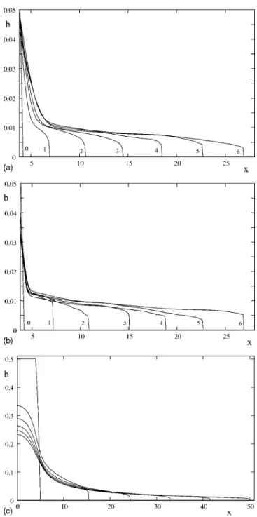
The results of the numerical solution are presented in Figs. 5–7. The evolution of the magnetic induction is pre-sented in Fig. 5 for the following values of the flux and heat diffusion constant:共a兲 ⌽=0.5, ␬= 0.1,共b兲 ⌽=0.5, ␬= 0.01, and共c兲 ⌽=2.4, ␬= 0.05. The value of⌶_n was kept fixed at

⌶n= 0.5. Different curves represent successive times with

in-tervals of⌬t=2.5t*between them. Velocity of the sharp front

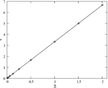
is constant and is plotted as a function of ⌶_n in Fig. 6 for

⌽=2.4 and ␬= 0.05. The temperature front moves together with the flux front velocity. The data are presented for the same times as for the magnetic induction. It demonstrates that the front interface velocity V is linearly dependent on

⌶n. The dependence of ⌽ is negligible. The results closely

follow Eq.共44兲 obtained analytically for␬= 0 and confirms the general physical picture proposed in the previous section that the velocity of the shock wave is universal in a sense

FIG. 5. The evolution of the magnetic induction for the flux conserving boundary condition. The value of the Joule heat released in the normal domain⌶n was kept fixed at ⌶n= 0.5. The curves correspond共from left to right兲 to six different times with intervals of ⌬t between them. 共a兲 The flux ⌽=0.5 and the heat diffusion constant ␬=0.1, ⌬t=2.5 t*_{. 共b兲 ⌽=0.5, ␬=0.01, ⌬t=2.5 t}*_{. 共c兲} ⌽=2.4, ␬=0.05, ⌬t=5 t*_.

that it depends only the heat released in the normal domain. The simulation reveals that the evolution is qualitatively the same for other values of the parameters.

The dynamics of the temperature distribution ␪共x,t兲 is presented in Fig. 7 and has a form of a thermal shock wave. Two sets of parameters were simulated:共a兲 ⌽=0.5, ␬= 0.1, and共b兲 ⌽=0.5, ␬= 0.01. The maximum of temperature␪in this wave is reached at the interface between the supercon-ducting and normal domains in the vicinity of the magnetic flux front. As we discussed in the previous section, the cur-rent is maximal in the normal domain which is narrow. We found in all the cases studied that the Joule heat released in the mixed state domain共see Fig. 4兲 does not exceed 1% of that in the normal domain. Note a curious feature of Fig. 7 that all the curves intersect at a certain point.

IV. GENERALIZATIONS: THE␮Å0 RESISTIVITY AND THE CONSTANT MAGNETIC FIELD BOUNDARY

CONDITION A. More general I–V␮Å0

Although in real samples resistance in the resistive mixed state might be a more complicated function than it was as-sumed earlier, the model representation in the form of Eqs.

共7兲 and 共8兲 with arbitrary critical exponents ␯ and ␮ is a robust and experimentally justified way to treat the problem. In such a case the main conclusions obtained for resistance with␮= 0, remain valid for some special relations between the critical exponents only.

Assuming bsand⌬sin the vicinity of the front共X→0兲 in

the form of the Eqs.共25兲 and 共26兲 one obtains asymptotically for A共V兲 and␣: ␣=␮+ 1 ␯+␮; A共V兲 = ⌬s0V 1/共␯+␮兲

冉

␮+ 1 ␮+␯

冊

−共␮+1兲/共␮+␯兲 . 共48兲

The electric current now behaves as

j⬀ 兩X兩共1−␯兲/共␮+␯兲 共49兲

and still diverges for␯⬎1. This condition is independent of ␮, although the power in Eq.共49兲 depends on␮. In the case ␯⬍1 there is no normal domain and one can neglect the

Joule heat. Hence, the temperature gradients are small and it suffices to consider the flux dynamics described by Eq.共15兲 with temperature fixed at␪0. Looking for an exact solution in a form

b = b₁t−␣_{f共␨兲, 共50兲}

where␨= b₂x / t␤, we obtain for b₁ and f共␨兲 共see Refs. 7 and 19兲, under the flux conservation law boundary condition ⌽ =兰dxb共x,t兲:

␣=␤= 1/共2␮+ 2 +␯兲; b1=⌽共␮+2兲/共2␮+2+␯兲;

b2=⌽−共␯+␮兲/共2␮+2+␯兲,

FIG. 6. Front velocity as a function of the Joule heat released in the normal domain⌶n. Here the flux is⌽=2.4, the heat diffusion constant is␬=0.05. Squares correspond to the simulated values of

⌶n, while the straight line is the analytical result.

FIG. 7. The evolution of the temperature profile for the flux conserving boundary condition. The value of the Joule heat released in the normal domain.⌶n was kept fixed at ⌶n= 0.5. The curves correspond to six different times with intervals of ⌬t=2.5 t*

be-tween them.共a兲 The flux ⌽=0.5 and heat diffusion constant is␬ = 0.1.共b兲 ⌽=0.5, ␬=0.01.

f共␨兲 =

再

冉

␮+␯ ␮+ 2

冊冉

1 2␮+ 2 +␯

冊

1/共␮+1兲 ␨f共␮+2兲/共␮+1兲 ⫻

冋

1 −

冉

␨ ␨f

冊

共␮+2_Ⲑ共␮+1兲

册

冎

共1+␮_Ⲑ共␮+␯兲 , 共51兲 ␨f −共2␮+␯+2Ⲑ共␮+␯兲₌␮+ 1 ␮+ 2

冉

␮+␯ ␮+ 2

冊

共共␮+1_Ⲑ共␮+␯兲 ₁ 关2 + 2␮+␯兴1/共␯+␮兲 ⫻B

冋

2 + 2␮+␯ ␮+␯ , ␮+ 1 ␮+ 2

册

, 共52兲

where B is the beta function. The flux front moves with velocity Vf共t兲=dxf/ dt⬀t␤−1 decaying with time. In the

ab-sence of the excessive heat released at the flux front the flux front in this case is completely stable.

B. Constant magnetic field

In certain cases similar phenomena will occur when flux is not conserved. Examples include narrow stripes, fields larger than Hc1, etc. This does not mean that the effect

dis-appears since magnetic flux generally forms a thermomag-netic shock wave. The main prerequisite is a phase transition from superconductor to normal metal resulting in a sharp flux front. This case was studied numerically for constant magnetic field共in units of B*_{兲 b=0.05 and parameters␯= 5,} ␬= 0.05,⌫=0, and ⌶=0.5. The profile of the magnetic field and the temperature shock waves are presented in Figs. 8共a兲,8共b兲, where different curves correspond 共from left to right兲 to various times: t=0, 5, 10, 15…共in the t*_{units兲. It is} important to note that, when the simulation was done for different⌶, the dependence was linear like for the constant flux in Fig. 6. This is consistent with our analytic result pre-dicting that the front velocity is governed solely by the Joule heat released in the normal domain. Other features are also independent of boundary conditions.

V. INSTABILITY OF THE STRAIGHT FRONT A. Linear stability analysis for␬=⌫=0

The dependence of the front velocity on the Joule heat released near the interface can lead to an instability of the straight front. Perturbations like a slight spatial distribution of the sample parameters共resistance, for example兲 can trig-ger the front instability. Keeping the normal resistivity in the form ␳n=␳0+␳1␪共x,t兲 we look for a solution of the corru-gated front in the normal domain as

b = b_n共x − Vt兲 +␩共x,y,t兲,

␪=␪n共x − Vt兲 +␨共x,y,t兲. 共53兲

The leading order solution␤nand␪nfor the set of basic Eqs.

共15兲 and 共16兲 for␳1= 0 were obtained in Sec. III, while cor-rections to the first order in ␳1 will not be required in the stability analysis. The first order terms in perturbations␩and ␨are ⳵␩ ⳵t =␳n共␪n兲ⵜ 2_␩+␳ 1 ⳵␪n ⳵x ⳵␩ ⳵x+␳1 ⳵2_b n ⳵x2␨+␳1 ⳵bn ⳵x ⳵␨ ⳵x, 共54兲 ⳵␨ ⳵t = 2␳n共␪n兲 ⳵bn ⳵x ⳵␩ ⳵x+␳1

冉

⳵bn ⳵x

冊

2 ␨. 共55兲

Due to translation invariance of these eigenvalue equations in time and the direction along the front y one represents␩,␨ in a form

␩=␩共x兲exp共⍀t + kyy兲; ␨=␨共X兲exp共⍀t + kyy兲. 共56兲

Then the eigenvalue equations become one dimensional

Lˆ

冋

␩

␨

册

=⍀

冋

␩

␨

册

, 共57兲

where

FIG. 8. Magnetic field at x = 0 is constant. The curves corre-spond to six different times from left to right with intervals of⌬t = 5 t*between them. Joule heat released at the front⌶=0.5. 共a兲 The magnetic induction evolution and共b兲 the temperature shock wave.

共58兲

Let us first consider the simpler case of conventional super-conductors for which␳1= 0. Substituting Eqs.共35兲,共36兲 into Eqs.共54兲 and 共55兲 one obtains 关replacing 共⳵/⳵X兲→ikX兴:

共59兲

The matrix Lˆ0has one stable⍀1= −␳0共kX

2_{+ k}

y

2_{兲 and one} mar-ginal⍀2= 0 eigenvalues. This eigenvalue is highly degener-ate: any temperature deviation ␨ for ␩= 0 belongs to this subspace: Lˆ₀

关

0_␨

兴

= 0. Strictly speaking the marginal eigen-value ⍀2 calls for investigation beyond the linear stability analysis. However, we believe it is stable and, in any case, addition of the␳1term to resistivity removes the marginality and the degeneracy. To find the corrected eigenvalue⍀₂, one has to diagonalize on the corresponding subspace the opera-tor Lˆ_␨␨=␳1

冉

⳵bn ⳵X

冊

2 . 共60兲

The derivative is nearly constant in the normal domain, see Eq.共35兲: Lˆ_␨␨=␳1jn0 2 _exp

冋

₋2XV ␳n

册

⬇␳1jd 2_{. 共61兲} Consequently ⍀2=␳1jd 2 , 共62兲

which demonstrates the instability for any wave vector. The physical reason for the instability is the positive feed-back between temperature fluctuation at the front increasing in its turn both the Joule power at the front and its velocity. In fact, it is the well known hydrodynamics tangential instability20 _{of the flux front which is responsible for the} front instability. Indeed, in this case warmer segments of the front move faster and can destroy the flat front line.

B. Stability in the general case: Numerical simulation If the normal resistivity of the sample is temperature de-pendent and ␬=⌫=0, then the normal domain in the front shows instability with respect to small temperature fluctua-tions with arbitrary wave vector. In this case the normal do-main in the front shows instability with respect to small tem-perature fluctuations with arbitrary wave vectors. The dispersion appears for the nonzero heat diffusion coefficient. In fact, however, these small fluctuations cannot destroy the straight line front. It becomes unstable due to large amplitude fluctuations. Let us consider the evolution of the instability.

First of all the instability can develop when the characteristic time t0⯝1/共␳1jd

2_{兲 is smaller than the characteristic time of} the heat absorption in the sample tr⬇⌫−1. In addition the

heat diffusion along the y axis can also affect the unstable fluctuations. In the latter case the requirement is: ut0⬎

冑

␬t0. These two requirements allow us to determine the critical velocity of the fluctuation for the onset of the instability

u⬎ uc= min兵⌫wn, jd

冑

␬␳1其. 共63兲 In metals and alloys the normal state resistivity practically does not depend on temperature in the relevant temperature range. This means that␳₁= 0 and consequently no instability is expected.

The threshold in the fluctuation velocity uc共which is

pro-portional to the Joule heat released in the front兲 means that only a large temperature fluctuation can provide Joule heat-ing necessary to destroy the planar front. Physically large amplitude fluctuations of the temperature at the front are nonuniform because they are caused by the spatial distribu-tion of the impurities in the sample locally increasing resis-tivity and hence the Joule heat and velocity of the fluctua-tions in the front. Numerical simulafluctua-tions support this scenario.

In order to study the development of the instability for arbitrary ␬, the set of the Eqs. 共15兲,共16兲 have been solved numerically. The Joule heat power⌶_nreleased in the normal domain at the front has the following model form:

⌶n共␪兲

⌶n0

⬅␳n共␪兲

␳0

= 1 +␣关␪共x,y,t兲 −␪0兴, 共64兲 where initial temperature is perturbed in the region 0⬍x

⬍5, 4⬍y⬍5, 共temperature fluctuation ␪共x,y,t=0兲=0.88兲,

while outside this region␪共x,y,t=0兲=␪0= 0.7. We chose␣ = 14.5, ␬= 0.05 and 2.5. Physically this kind of fluctuation represents a local variation of the normal state resistivity

共proportional to ⌶n兲 when the front of the shock wave passes

an inhomogeneity.

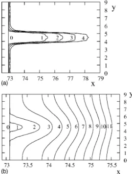
The evolution of a small fluctuation in two opposite limits is presented in Fig. 9. For small ␬, Fig. 9共a兲, an unstable pattern of the magnetic induction develops. It should be noted that the flux front line lost its stability essentially im-mediately after the temperature fluctuation affected the sys-tem. For finite␬ we observe that most of the␬= 0 unstable modes are diffused away and do not develop into an insta-bility of the system. For large␬, Fig. 9共b兲, a similar pertur-bation relaxes into a straight line front and disappears in accord with the stability analysis.

VI. DISCUSSION

To summarize, we considered the formation and stability of the shock waves in the vortex matter under extreme con-ditions of the fast flux expansion into the Meissner state. In this case very strong screening currents significantly exceed-ing the critical current J_c flow in the mixed state. For such strong currents the vortex matter resistivity R has a form R

⬀B␯_J␮_{. We predict that when␯⬎1 both the moving flux and}

Strong screening currents in the vortex matter approaching the depairing current J_dcause destruction of superconductiv-ity. An area of material adjacent to the interface between the Meissner state and the mixed state of the size共returning to dimensional units兲 Wn=关cB*共1−T0/ Tc兲/4␲␯Jd0兴 becomes

normal. Here B*₌

冑

_4␲CT

c, C is the heat capacity and T0 is temperature of the cool superconductor. The stable superconductor-normal interface is formed due to combined effect of the nonlinear magnetic flux dynamics and thermal effects. The condition␯⬎1 is independent on␮and has the following physical meaning. It is well known that above the critical current resistivity is proportional to the number of vortices 共the flux flow Bardeen-Stephen formula兲, R⬀B共 ␯ = 1兲. The condition for formation of the normal domain is therefore that the dependence on magnetic induction at cur-rents close to the depairing curcur-rents is stronger than linear. As was shown in Sec. II B for Nb, this happens at least for small fields.

The interface moves with constant velocity, which is completely determined by the Joule heat released in the normal domain at the front and hence on the normal

resistiv-ity of the sample. The flux front velocresistiv-ity has the form for ␮= 0 共in dimensional units兲 is V=关cRnJd0/共1−T0/ Tc兲B*兴

⫻关B*_{/ B}

c2共0兲兴␯ . Taking for example material parameters of

the optimally doped YBCO, Jd0= 108A / cm2, Rn

= 2 · 10−6 _{⍀ cm, C=1 J/cm}3_K,21 _{one obtains for the flux} front velocity V⬇105_{cm/ s, which is in a good agreement} with experimental data.12 _{Note, however, that the value} strongly depends on the exponents␮and␯. The width of the normal stripe is 0.5␮m.

The type of the voltage–current characteristic therefore is the decisive factor determining the flux front stability in type-II superconductors. The instability is developed when the voltage–current characteristics of the uniform supercon-ductor in its resistive state provides sufficient screening cur-rents at the moving flux front interface. The physical reason for the instability is very similar to a well known hydrody-namic instability,20_{when different layers of the liquid move} with different and parallel velocities. In fact it is the positive feedback between excessive local temperature at the front and Joule heat released there that leads to instability. The hydrodynamic tangential instability of the flux front destroys the flat front. The instability develops for the fluctuation ve-locities exceeding the critical value U⬎Uc= min兵关cB*共1

− T0/ Tc兲/4␲␯Jd0tr兴,共Jd0/ C兲

冑

D兩共dRn/ dT兲兩T_c其, where D is the

heat diffusion constant and tr is the heat absorption time.

Taking D = 30 J /共cm s K兲 and t_r= 10−11_{s, one estimates the} two velocities as 5 · 106 _{cm/ s and 2.6· 10}5_{cm/ s.}

The avalanche-type instability appears when the moving flux front enters the area in which locally the normal resis-tivity is large. The experimental observation of the fast flux dynamics in YBCO has been carried out by Leiderer et al.12 The velocity of the front indeed has the universal character on the advanced stage of the instability and does not depend on initial magnetic gradients. The dendrite velocity in the later stages of disintegration of the front are expected to be of order of U_c. This instability is not expected to arise in materials like Nb since 兩dRn/ dT兩T_cis negligibly small and Uc

vanishes.

ACKNOWLEDGMENTS

We are grateful to D. Kessler, Y. Yeshurun, Y. Rabin, A, Shaulov, and H. H. Wen for discussions and V. Vinokur for his criticism. This work was supported by The Israel Science Foundation, ESF Program “Cosmology in the Laboratory.” We are also grateful to the Binational Israel-USA and Germany-Israel Foundations for support and to the Inter-University Computational Center for providing Cray J932 supercomputer facilities. B.R. acknowledges Albert Einstein Minerva Center for Theoretical Physics in Weizmann Insti-tute and NSC grant ROC94-2112-M009-024 of R.O.C. and the hospitality of Bar Ilan University.

FIG. 9. Evolution of the magnetic flux front pattern for different values of the heat diffusion constant. The perturbation is triggered by the temperature inhomogeneity specified in Eq.共64兲. 共a兲 Small heat diffusion constant␬=0.05. Development of the avalanche in-stability. Five snapshots共intervals of ⌬t=0.05 t*_{兲 of a finger shaped}

instability in magnetic induction are shown from left to right.共b兲 Large heat diffusion constant␬=2.5. Evolution of the magnetic flux pattern. The five snapshots共intervals of ⌬t=0.125 t*兲 show that the initial small fluctuation dissipates away.

*Author to whom correspondence should be addressed.

1_{R. G. Mints and A. I. Rahmanov, Rev. Mod. Phys. 53, 551} 共1981兲; A. V. Gurevich, R. G. Mints, and A. I. Rahmanov, The Physics of Composite Superconductors 共Begell House, NY,

1997兲.

2_{L. A. Dorosinskii, M. V. Indenbom, V. I. Nikitenko, Yu. A.}

Os-sipyan, A. A. Polanskii, and V. K. Vlasko-Vlasov, Physica C

203, 149共1992兲.

3_{V. K. Vlasko-Vlasov, V. I. Nikitenko, A. A. Polyanskii, G. M.}

Crabtree, U. Welp, and B. W. Veal, Physica C 222, 361共1994兲.

4_{M. E. Gaevski, T. H. Johansen, Yu. Galperin, H. Bratsberg, A. V.}

Bobyl, D. V. Shautsev, and S. F. Karmarenko, Appl. Phys. Lett.

71, 3147共1997兲.

5_{C. A. Duran, P. L. Gammel, R. E. Miller, and D. J. Bishop, Phys.}

Rev. B 52, 75共1995兲.

6_{C. P. Poole, H. A. Farrah, and R. J. Creswick, Superconductivity} 共Academic Press, San Diego, 1995兲.

7_{F. Bass, B. Ya. Shapiro, and M. Shvartser, Phys. Rev. Lett. 80,}

2441共1998兲.

8_{A. Gurevich, Phys. Rev. B 46, 3638共1992兲.}

9_{L. M. Fisher, P. E. Goa, M. Baziljevich, T. H. Johansen, A. L.}

Rakhmanov, and V. A. Yampol’skii, Phys. Rev. Lett. 87, 247005

共2001兲.

10_{P. Leiderer, J. Boneberg, P. Brull, V. Bujok, and S. Herminghaus,}

Phys. Rev. Lett. 71, 2646共1993兲; U. Bolz, J. Eisenmenger, J. Schiessling, B.-U. Runge, and P. Leiderer, Physica B 284-288,

757共2000兲; U. Bolz, D. Schmidt, B. Biehler, B.-U. Runge, R. G. Mints, K. Numssen, H. Kinder, and P. Leiderer, Physica C

388-389, 715共2003兲.

11_{I. Shapiro, E. Pechenik, and B. Ya. Shapiro, Phys. Rev. B 63,}

184520共2001兲.

12_{U. Bolz, B. Biehler, D. Schmidt, B. U. Runge, and P. Leiderer,}

Europhys. Lett. 64, 517-523共2003兲.

13_{V. M. Vinokur, M. V. Feigelman, and V. B. Geshkenbein, Phys.}

Rev. Lett. 67, 915共1991兲.

14_{F. Bass, B. Ya. Shapiro, I. Shapiro, and M. Shvartser, Physica C} 297, 269共1998兲; 297, 269 共1998兲.

15_{F. Bass, B. Ya. Shapiro, and M. Shvartser, Phys. Rev. Lett. 80,}

2441共1998兲; I. Aranson, A. Gurevich, and V. Vinokur, ibid. 87, 067003共2001兲.

16_{C. Villard, C. Peroz, and A. Sulpice, J. Low Temp. Phys. 131,}

957共2003兲.

17_{B. Kalisky, G. Koren, A. Shaulov, Y. Yeshurun, and R. P.}

Hue-bener共unpublished兲.

18_{L. Burlachkov, D. Giller, and R. Prozorov, Phys. Rev. B 58,}

15067共1998兲.

19_{D. Zwillinger, Handbook of Differential Equations, 3rd ed.}

共Aca-demic Press, Boston, 1997兲, p. 424.

20_{L. D. Landau and E. M. Lifshitz, Fluid Mechanics, Course of}

Theoretical Physics Vol. 6共Pergamon Press, New York, 1980兲.

21_{M. Aravind and P. C. W. Fung, Meas. Sci. Technol. 10, 979} 共1999兲.