Attribute selection for neural network-based adaptive scheduling systems in flexible manufacturing systems

Int J Adv Manuf Technol (2002) 20:532–544 Ownership and Copyright

 2002 Springer-Verlag London Limited

Attribute Selection for Neural Network-Based Adaptive

Scheduling Systems in Flexible Manufacturing Systems

Y.-R. Shiue

_{and C.-T. Su}

1_{Department of Industrial Management, Van Nung Institute of Technology, Chungl, Taiwan;}2_{Department of Industrial Engineering and} Management, National Chiao Tung University, Hsin-Chu, Taiwan

System attribute selection is an integral part of adaptive sched-uling systems. Owing to the existence of irrelevant and redun-dant attributes in manufacturing systems, by selecting the important attributes, better performance or accuracy in predic-tion can be expected in scheduling knowledge bases. In this study, we first propose an attribute selection algorithm based on the weights of neural networks to measure the importance of system attributes in a neural network-based adaptive scheduling (NNAS) system. Next, the NNAS system is combined with the attribute selection algorithm to build scheduling knowledge bases. This hybrid approach is called an attribute selection neural network-based adaptive scheduling (ASNNAS) system. The experimental results show that the proposed ASNNAS system works very well, when measured by a variety of per-formance criteria, as opposed to the traditional NNAS system and a single dispatching strategy. Furthermore, the scheduling knowledge bases in the ASNNAS system can provide a stronger generalisation ability compared with NNAS systems under vari-ous performance criteria.

Keywords: Adaptive scheduling; Attribute selection; Flexible

manufacturing systems; Knowledge based systems; Learning by example; Neural network

1.

Introduction

A flexible manufacturing system (FMS) is a highly automated and computer controlled system that produces parts of moderate volume and variability. FMS’s have already demonstrated a number of benefits in terms of time reduction in production cycle, high product quality, high equipment utilisation, and greater flexibility in production scheduling, etc. An important property of an FMS is that it can handle higher uncertainty in the manufacturing processes such as machine breakdown, random change of product mix, flexible routeing, and different Correspondence and offprint requests to: Dr C.-T. Su, Department of

Industrial Engineering and Management, National Chiao Tung Univer-sity, 1001 Ta Hsueh Road, Hsin-Chu, Taiwan. E-mail: ctsu얀cc.nctu.edu.tw

customer demand criteria, etc. Therefore, the profitability of using a capital-intensive FMS depends on the ability to control it efficiently. In order to make the task of controlling an FMS more effective, the system is usually divided into a task-based hierarchy. One of the standard hierarchies that has evolved is the factory real-time production control hierarchy in a dynamic manufacturing environment proposed by the National Institute of Standards and Technology (NIST) [1]. An automated manu-facturing research facility (AMRF) has been developed to demonstrate these concepts. The key to successful implemen-tation of an AMRF model is its hierarchical planning and control structure, its transparency, and the partition of the management, planning, and control functions.

Many workers [2–5] believed that the development of an efficient scheduling mechanism is the core of FMS operational control functions. Thus, it becomes necessary to use the system resources in the most effective manner when building a sophis-ticated scheduling mechanism.

In dynamic uncertain manufacturing environments, schedul-ing decisions are usually implemented through dispatchschedul-ing rules that assign priority indices to the various jobs waiting at a machine; and the job with the highest priority currently avail-able is performed next. Many workers [6–9] have studied dispatching rules in a variety of configurations since the 1960s; they have come to the conclusion that no single dispatching rule has been shown to produce better results consistently than other rules under a variety of shop configuration conditions and operating criteria.

Baker [7] suggested that it would be possible to improve system performance by implementing a scheduling policy rather than a single dispatching rule. Since the values of these attributes change continually in a dynamic system, it appears natural to use an approach that employs different scheduling heuristics adaptively at various time points. Based on this viewpoint, in order to resolve scheduling problems in real-time in an FMS environment, the scheduling function applies an appropriate dispatching rule each time that a decision problem is encountered. Instead of using a single dispatching rule for an extended planning horizon, the scheduling function changes dispatching rules on the basis of the current machine status over a series of short-term decision-making periods. This

tech-nique is called adaptive scheduling because it should be poss-ible to discover the current status of the manufacturing system, and it should then be possible to determine the most appropriate dispatching rule to be used for the next scheduling period. The following sections will examine the work on adaptive scheduling system.

There are three approaches to solving the problems of an adaptive scheduling system: the multi-pass simulation approach; the decision-tree learning approach; and the neural network approach. For the multi-pass simulation approach, Wu and Wysk [10] developed a multi-pass simulator methodology for the on-line control and scheduling of an FMS. A multi-pass simulator control mechanism evaluates the candidate dis-patching rules and selects the best strategy based on information such as the current system status, scheduling objective, and management goals for each short time period. In the long run, the control mechanism combines various dispatching rules in response to the dynamic behaviour of the system.

In the decision-tree learning approach, Shaw et al [11], Park et al. [5], and Arzi and Iaroslavitz [12] employed inductive inference algorithms to derive heuristics for selecting the appro-priate dispatching rules in an FMS. This approach uses a set of training examples, each of which consists of a vector of system attribute values and corresponding dispatching rules that are generated by simulation to construct the scheduling knowledge in the form of a decision tree. By decision-tree learning, the suggested procedure provides the scheduler with the capability of selecting dispatching rules adaptively in a dynamic changing manufacturing environment.

Neural networks as learning tools have demonstrated their ability to capture the general relationship between variables that are difficult or impossible to relate to each other analytically by learning, recalling, and generalising from training patterns or data. In the neural network approach applied to adaptive sched-uling [2,13,14], a neural network constructed for a set of training samples (such as decision-tree learning training samples) can suggest a preference indicator for all the dis-patching rules for a given system status. A neural network, used as the rule selector, suggests one rule based on the current system status. In other words, the neural network plays the role of a dispatching rule decision maker that produces a rule suitable for the given system status.

Among the three approach discussed above, the multi-pass simulation approach is not well suited to on-line scheduling and control owing to its requirement for extensive effort in compu-tation to select the best dispatching rule. Therefore, machine learning approaches such as decision trees or neural networks become the major methodology employed in recent work.

No matter which one of the machine learning approaches is used to construct scheduling knowledge bases, the way that the training examples are described will affect the performance of the scheduling knowledge bases. A set of training examples is provided as input for learning the concept representing each class. A good training example must contain adequate information in a suitable form for the problem domain. If training examples do not carry the necessary information, or appropriate display information, they will have a negative effect on building the knowledge bases. In scheduling knowledge bases, a given training example consists of a vector of system

attributes and the corresponding best dispatching rule for spe-cific performance criteria. There are a large number of system attributes in a manufacturing system, so the system attributes which really reflect the current manufacturing system’s ability to meet performance criteria should be carefully determined. If we omit one important system attribute, it will have a strong effect on the learning performance, and may degrade the scheduling knowledge mapping ability.

Siedlecki and Sklansky [15] gave an overview of combina-torial feature selection methods and described the limitations of methods such as artificial intelligence (AI) methods for graph searching techniques or branch and bound search algor-ithms, and indicated their infeasibility for large-scale problems (they considered a 20-element selection problem to be in the large-scale domain). To handle large-scale problems they described the potential benefits of Monte Carlo approaches such as simulated annealing and genetic algorithms (GA). A direct approach to using GAs for attribute selection was intro-duced by Siedlecki and Sklansky [16]. In their work, a GA is used to find an optimal binary vector. Each resulting subset of features is evaluated according to its classification accuracy on a set of testing data using a nearest neighbour classifier. Nevertheless, their proposed methods are not suitable for a neural network-based classifier owing to the neural network’s architecture and because its learning parameters are determined empirically and cannot be resolved beforehand.

In the adaptive scheduling problem domain, Chen and Yih [17] proposed a neural network-based approach to identify the essential attributes for a knowledge-based scheduling system. In their approach, a penalty function was proposed to measure how much the performance of the network degrades from the upper bound of the performance when the information of an attribute is omitted. The major conclusion of their experiment is that scheduling knowledge bases using a set of selected attributes are superior for choosing desired dispatching rules under unknown production conditions, compared with the knowledge bases built by other sets of attributes. A weakness of their approach is that the attribute reduction process requires extensive computational effort and each dispatching rule has an equal weight in the significant score function when being chosen for the next control period. Chen and Yih [18] proposed a FSSNCA (feature subset selection based on nonlinear corre-lation analysis) procedure not only to select essential attributes, but also to generate important attributes to facilitate the devel-opment of knowledge bases and enhance the generalisation ability of the resulting knowledge bases. However, this FSSNCA procedure is not suitable for neural network-based scheduling systems.

The objective of this study is to develop a neural network-based adaptive scheduling system through selecting significant system attributes. This is called an attribute selection neural network adaptive scheduling (ASNNAS) system. The proposed approach possesses an advantage in terms of computation effort involved and outperforms the traditional neural network adaptive scheduling (NNAS) system under various production performance criteria. In addition, it can more accurately predict dispatching strategy for the next scheduling control period.

This paper is organised as follows. In Section 2, we give some background information about neural networks and

dis-cuss the literature related to input neuron selection in neural networks. In Section 3, we describe the framework of the proposed ASNNAS system. In Section 4, we describe the model considered, and define the set of training examples in this study. In Section 5, we implement an ASNNAS system for an FMS case problem and some simulation results are discussed. Finally, in the last section, we summarise some conclusions and future research issues.

2.

Background Information

2.1 Artificial Neural Network

Artificial neural networks (ANNs) are simplified models of the central nervous system. They are networks of highly intercon-nected neural computing elements that have the ability to respond to input stimuli and to learn to adapt to the environ-ment. In ANNs, the use of distributed, parallel computations is the best way to overcome the combinatorial explosion. ANNs are good at tasks such as pattern matching and classi-fication, function approximation, optimisation, and data clus-tering.

2.1.1 Back Propagation Learning Algorithm

In this study, a back propagation (BP) network as shown in Fig. 1 is chosen to develop the proposed model. BP networks have been used successfully in many on-line adaptive schedul-ing tasks described in the literature as well as in many other applications [19]. Although the training of a BP network-based systems tends to be relatively slow, the recall process is fast. This is acceptable, as the primary interest of this study is to propose a neural network adaptive scheduling system that can be applied in on-line mode, but will be trained off-line. In addition, most attribute selection methods are provided by BP networks in the literature, so we believe that a BP network suits this study.

A BP network is composed of several layers of neurons: an input layer, one or several hidden layers, and an output layer. Each layer of neurons receives its input from the previous layer or from the network input. The output of each neuron feeds the next layer or becomes the output of the network. The above statement can be represented by the following mathematical equations:

Fig. 1. The BP network structure.

netpj⫽ i苸_previous

冘

冉

冊

where wij is the weight from neuron i to neuron j; bjis a bias

associated with neuron j; apj is the activation value of neuron

j with a sigmoid function for pattern p.

The application of a BP network requires a learning pro-cedure, which gradually adjusts the neural weights until the network correctly maps all the training inputs onto the corre-sponding training outputs. In order to decrease the global error, this can be done using the gradient-descent rule as follows:

⌬wij⫽ ␩

⭸E ⭸wij

(3) where ␩ is learning rate, and E is the global error function.

From Eq. (3), the change in weight is proportional to the magnitude of the negative gradient of E. The global error function is the objective of the minimising procedure and is defined as follows:

E⫽ 1

2p

冘

冘

layer

(tpk⫺ opk)2 (4)

where tpk is the target of the kth output neuron when the pth

pattern is presented; opk is the actual output of the kth output

neuron when its pth pattern is presented.

One of the problems of a gradient-descent rule is setting an appropriate learning rate. The gradient-descent can be very slow if the learning rate ␩ is small and can oscillate widely if ␩ is too large. This problem results essentially from error-surface valleys with steep sides but shallow slopes along the valley floors. One efficient and commonly used method that allows a greater learning rate without causing divergent oscil-lations is the addition of a momentum term to the normal gradient-descent method. The idea is to give each weight some momentum so that it will tend to change in the direction of the average downhill force that it feels. This scheme is implemented by giving a contribution from the previous time step to each weight change:

⌬w(t) ⫽ ⫺␩ⵜE(t) ⫹ ␣⌬w(t ⫺ 1) (5)

where ␣ ⑀ [0, 1] is a momentum parameter and a value of 0.9 is often used.

2.1.2 Network Architecture

At present, there is no established theoretical method to deter-mine the optimal configuration of a BP network. Most of the design parameters are application-dependent and must be determined empirically. Patterson [20] indicated that a single hidden layer would be sufficient for most applications. A second hidden layer will improve the performance when the mapping function is particularly complex or irregular. The need for more than two hidden layers is highly unlikely. In this study, the proposed BP network consists of three layers: one input layer, one hidden layer, and one output layer. In the

BP network-based adaptive scheduling model, the input layer contains some user-determined neurons that represent system state attributes, one neuron for each state attribute. The neurons of the output layer are determined by the dispatching rules considered as shown in Fig. 1.

Once the number of input and output neurons is established, the number of hidden units should be determined next. Widrow et al. [21] indicated that the optimal number of hidden neurons could be determined by trial and error. The best way is to start with an estimation of the minimum number and refine the network by adding and pruning neurons. When deciding on the appropriate number of neurons to start with for a given application, we can use the rule-of-thumb that the number of neurons h in the first hidden layer should be about

h⫽ P

10(m⫺ n) (6)

where P is the number of training examples and n and m are the number of inputs and outputs, respectively.

2.1.3 Data Pre-processing

Before the data are presented to the networks, all of the values of input neurons are usually normalised to the range of [⫺3, 3], and the values of output neurons are normalised to the range of [0, 1]. The reasons are as follows. First, in a BP network, if the value of the input pattern is greater than 3, the result of the sigmoid function will be close to 1; and if the value of the input layer is less than ⫺3, the result of the sigmoid function will be close to 0. Thus, too many values of the input pattern which are greater than 3 or less than ⫺3 will impede the change in the weights of the BP network. Secondly, for the BP network, the value of the target pattern in the sigmoid function should be set between 0 and 1. The values of training examples in the pre-processing equations used in this study are defined as follows:

S⫽High⫺ Low

Max⫺ Min (7)

O⫽Max⫻ Low ⫺ Min ⫻ High

Max⫺ Min (8)

Xadj⫽ S Xin⫹ O (9)

where Xin is the input value of training examples; Xadj is the

adjusted value after normalisation of the training examples; S and O are scale and offset values, respectively. Max and Min are the actual maximum and minimum values of each input or output node in all training examples, respectively. High and

Low are the desired maximum and minimum values for input

or output patterns in all training examples, respectively.

2.1.4 Network Learning

Once the basic network architecture has been established, the details of the training process and training regime can be determined. The initial weights of the BP network are randomly set between ⫺0.5 and ⫹0.5. For training, the standard back-propagation learning algorithm can be used. In this case, the best performance can be achieved by varying the learning and momentum coefficients during the training process. Based on

experimental experience, the value of ␩ can be set low 0.20– 0.25) at the beginning, then by gradually increasing the value of␩, we can find a suitable learning rate. On the other hand, the value of ␣ can be set high (0.90–0.95) at the beginning, then by gradually increasing the value of ␣, we can find an appropriate momentum coefficient.

The training set should be divided into two groups: a set for training the network, and a set for testing the performance of the trained network. The training and testing sets should be of approximately equal size if a sufficient number of samples are available. Otherwise, the training set should be given priority in order to ensure a good generalisation of training examples, the value of the root mean square (RMS) error defined in Eq. (10) for all patterns can be used as an index for the performance of the trained network. If the RMS error reaches a stable condition or is less than some criterion, the network stops training and then uses the testing data set to verify the trained networks. The network with the lowest RMS error can be selected as the final neural network.

RMS error⫽

冑

冪

冉

2P

冘

冘

(tpk⫺ opk)2

冊

2.2 Attribute Selection Algorithm Based on Weights of Neural Networks

The interconnections of all the neurons provide essential infor-mation on the BP network architecture. The weight wij

rep-resents the strength of the synapse (called the connection or link) connecting neuron i (source) to neuron j (destination). Positive weights have an excitatory influence, whereas negative values of weight have an inhibitory influence. Zero value in weights means no connection between the two neurons. In a BP network, the output of the network depends on both the weights of the input to the hidden layer and the weights of the hidden layer to the output; therefore, it is tempting to try to combine these two sets of weights in a measure of the importance of input neurons.

Based on the above viewpoint, several workers [22,23] proposed the following measure for the proportional contri-bution of an input to a particular output:

Qik⫽

冘

冢

冘

冘

冣

where i is the input layer neuron index; j is the hidden layer neuron index; k is the output layer neuron index; wij is the

weight from the input layer of neuron i to the hidden layer of neuron j; wjk is the weight from the hidden layer of neuron j

to the output layer of neuron k.

In order to capture scheduling knowledge, we must decide on a mapping function between system attributes and dis-patching rules under different performance criteria for the neural networks in this study. The measure for input neurons introduced here is an extension of Eq. (11). We can define attribute selection score of input neuron i by the equation below:

ASi⫽

冘

Qik

k (12)

where k is the output layer neuron index and also represents the dispatching rule used in this study.

In Eq. (12), a higher score means that the attribute for this input neuron is more important. A major problem is how many attributes should be used in a BP network model for training. The relevant work offers no definite answer. In this study, we set a threshold value that is equal to a reciprocal value of the studied attributes. If the attribute selection score is below this threshold value, the corresponding input neuron can be deleted from the BP model. Only when using important attributes as the inputs for neural networks, can a higher system performance or generalisation ability in scheduling knowledge bases be expected.

3.

The Architecture of the ASNNAS

System

The ASNNAS system shown in Fig. 2 has been designed to identify important attributes of the system status and then build scheduling knowledge bases for an FMS system. The concept of constructing this system is based on a neural network approach that learns relations from a set of training examples. The proposed ASNNAS system includes three stages: training example generation, attribute selection procedure, and on-line adaptive scheduling knowledge generation.

Fig. 2. The architecture of the ASNNAS system.

The first stage is to collect a set of training examples. The input data of this stage include the FMS system specification, production data specifications, the training example specifi-cation (to be described in Section 4), the training example collection mechanism, and the scheduling control period to build a simulation model for off-line learning training examples. In this stage, the training example collection mech-anism must provide a comprehensive initial knowledge base, which represents a wide range of possible system states. In order to reach this goal, we use the multi-pass simulation approach [10] as a mechanism for the collection of training samples.

The length of a scheduling control period may have an effect on the system performance [2,10]. If the scheduling control period is too short, no statistics can be collected for a given reasonable performance measure. On the other hand, if the scheduling control period is too long, the adaptive schedul-ing mechanism will not be sensitive enough to switch between different dispatching rules at correct time. Therefore, it would be better to determine the scheduling control period based on performance criteria in a dynamic manner.

The second stage is the attribute selection stage. In this stage, the set of training examples is put into the neural network for off-line learning. The task of the training phase is to determine the weights of neural networks so that the input/output (system attributes/dispatching rules) mapping func-tions can be captured by the neural network. When the values of network weights are generated, the attribute selection algor-ithm can then be employed to identify important system attri-butes. This stage results in a set of training examples with important attributes.

In the third stage, the neural network retrains the whole set of training examples with important attributes obtained from the second stage in order to generate scheduling knowledge bases. When neural network off-line learning finishes, the FMS system can receive the scheduling control period signal from the on-line adaptive scheduling control mechanism and then enter the current system status into the neural network for on-line scheduling control. The neural network-based adaptive scheduling control mechanism compares the forecast perform-ance measures of various output nodes (dispatching rules) and selects the best dispatching rule as the execution function for the next control period. In other words, the neural network in this stage plays the role of a decision maker that produces part dispatching strategies suitable for the current system status. Using this architecture, the ASNNAS system can easily identify important attributes for building sound adaptive scheduling knowledge bases, and the performance of the FMS system will be significantly improved in the long run.

4.

FMS Problem Description

4.1 Model Characteristics

Figure 3 shows an FMS model layout used in this study, which is a modification of the model used by Montazeri and Van Wassenhove [8]. The FMS system consists of three machine families (F1, F2, and F3), three load/unload stations,

Fig. 3. The layout of the FMS model in this study.

three AGVs, an input buffer and a central WIP buffer with limited capacity, and a computer-controlled local area network. The first two machine families have two machines, and the third family has one machine. There are 11 different types of part to be produced in this model. In order to achieve different conditions in terms of machine load and shifting bottleneck, we design five types of product mix ratios (as shown in Table 1), which will be changed continuously over a constant time period.

Several related operating assumptions are listed below. 1. It is assumed that the raw materials for each type of part

are readily available.

2. Each job order arrives randomly at the FMS and consists of only one part with an individual due date.

3. A part with a pallet travels to each machine or load/unload station in order to achieve operation flexibility, and the part type match for one specific pallet problem is not con-sidered.

4. Each machine can execute only one job order at a time. 5. Each machine is subject to random failures.

Table 1. Part mix ratio used in this study.

Part mix ratio (%)

Part ID Type 1 Type 2 Type 3 Type 4 Type 5

1 11.00 14.00 6.00 9.00 14.00 2 11.00 14.00 6.00 9.00 14.00 3 11.00 15.00 6.00 9.00 14.00 4 12.00 10.00 15.00 8.00 15.00 5 6.00 12.00 15.00 13.00 7.00 6 8.00 8.00 9.00 12.00 5.00 7 8.00 5.00 8.00 3.00 5.00 8 7.00 3.00 8.00 9.00 4.00 9 7.00 3.00 7.00 8.00 4.00 10 2.50 1.00 4.00 1.00 6.00 11 16.50 15.00 16.00 19.00 12.00

6. Processing times are assumed to be predetermined. 7. An idle machine in a family has a higher priority than

other machines to process a part. If there is no idle machine in the family, then the part goes to the machine of the lowest utilisation.

8. When the part finishes each step of the process, it must return to one of available load/unload stations for reorien-tation. Otherwise, it will go to central WIP buffer to wait for the next operation (part reorientation in load/unload stations).

9. An AGV can carry only one piece of a part at a time and move in the counterclockwise direction only.

10. All material movements not using the AGV system are assumed to be negligible.

Based on the assumptions discussed above, the part type, routeing, and process time are given in Table 2.

4.2 Training Examples Presentation

A set of training examples is provided as system information for learning the concepts representing each class. A given training example consists of a vector of attribute values and the corresponding class. A concept learned can be described by a rule determined by a machine learning approach such as inductive learning or by using a neural network. If a new set of input attributes satisfies the conditions of this rule, then it belongs to the corresponding class. Baker [7] indicated that the relative effectiveness of a scheduling rule depends on the state of the system, given by performance criteria. Hence, in order to build the scheduling knowledge bases, training examples must have enough information to reveal this property. In adaptive scheduling knowledge bases, a set of training examples can be represented by the triplet兵P, S, D其. P denotes the user-defined management performance criteria; S is the set of system status; D represents the best dispatching rule under this performance criteria and system status.

Three kinds of performance criterion are usually studied in adaptive scheduling research [2,5,11,12,14]: throughput based; flow-time based; and due-date based. In order to compare the efficiency of the ASNNAS system with that of other

dis-Table 2. Part routeing and process times.

ID Average time Part routeing Processing

per operation (min) times (min)

1 9.14 L F2 L F1 3 11 10 20 L F2 L 3 14 3 2 9.00 L F2 L F1 3 10 10 24 L F2 L 3 10 3 3 12.14 L F2 L F1 3 15 3 30 L F2 L 10 21 3 4 16.71 L F2 L F1 3 12 3 53 L F2 L 10 33 3 5 13.67 L F2 L F1 8 16 5 25 L F1 L F2 5 22 10 24 L 8 6 19.45 L F2 L F1 5 25 15 24 L F1 L F1 5 22 10 38 L F2 L 3 57 10 7 18.45 L F2 L F1 5 28 15 27 L F1 L F1 5 25 10 40 L F2 L 3 35 10 8 20.00 L F2 L F1 5 36 15 30 L F1 L F1 5 32 10 49 L F2 L 3 25 10 9 24.73 L F2 L F1 5 45 15 42 L F1 L F1 5 34 10 80 L F2 L 3 23 10 10 38.82 L F2 L F1 5 52 10 61 L F1 L F1 5 61 30 112 L F2 L 3 38 50 11 36.11 L F3 L F3 12 95 12 45 L F2 L F2 3 36 50 51 L 21

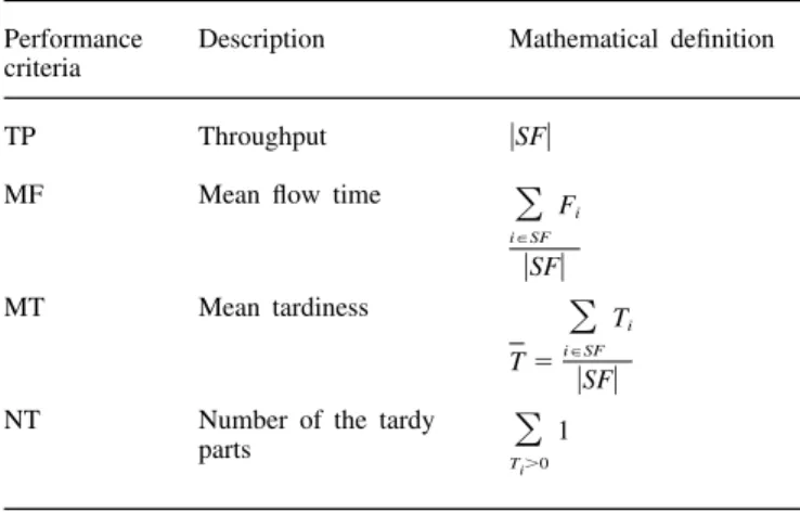
patching rules with respect to different performance criteria, the four performance criteria used in this study are shown in Table 3.

In the FMS environment, jobs arrive randomly and system attributes change over time. Because of the exponentially grow-ing complexity of the underlygrow-ing optimisation problem, sched-uling decisions in such systems are usually specified in terms of scheduling rules. Whenever a machine becomes idle, which job should be processed next on the machine must be determ-ined. This selection is made by assigning a priority index to various jobs competing for the given operation, the job with

Table 3. Performance criteria used in this study.

Performance Description Mathematical definition criteria

TP Throughput 兩SF兩

MF Mean flow time

冘

i苸SF Fi 兩SF兩 MT Mean tardiness T⫽i

冘

NT Number of the tardy

冘

Ti⬎0

1 parts

the highest priority is selected. Dispatching rules differ in how they assign these priority indices. The need for using adaptive dispatching rules arises from the fact that no single dispatching rule has been proved to be optimal for a job shop or an FMS environment. That is, no dispatching rule has been shown to produce consistently lower total costs than all other rules under a variety of shop configurations and operating conditions. For example, in the case of minimising tardiness, the shortest processing time (SPT) heuristic is found to be effective for high machine use and tight due dates, whereas the earliest due date (EDD) is effective when due dates are loose. The modified operation due date (MOD) delivers the best performance in the intermediate range and with a balanced workload. However, when significant imbalance in machine workload exists, the modified job due date (MDD) is suggested for implementation. Based on the statements discussed above, it is not necessary to spend excessive effort in studying the best dispatching heuristics in different environments. We select nine dispatching rules that have been found to be effective for the objective in terms of four performance criteria in this study. Table 4 gives these nine heuristic dispatching rules.

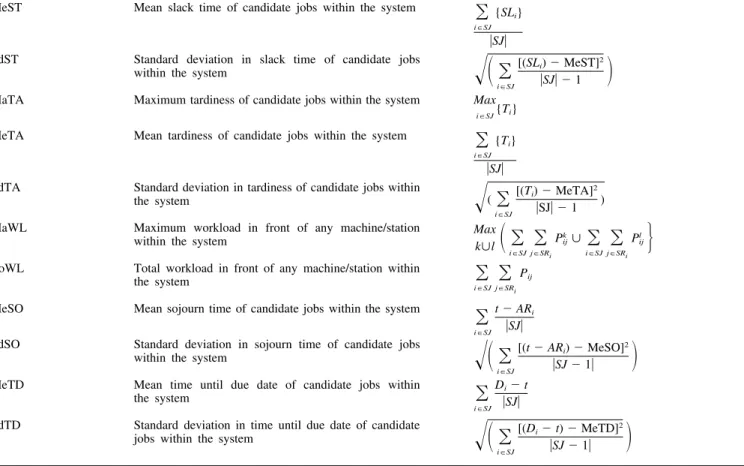
The major objective of this study is to identify important system attributes under different performance criteria, so, we try to examine exhaustively all possible system attributes. Thirty candidate attributes were examined and are given in Table 5. The selected criteria for system attributes are based on previous work [2,12,14,17,18], which used machine learning methodology to develop scheduling knowledge bases.

Table 4. FMS system attribute used in this study.

System attribute Description Mathematical definition

NJ Number of the jobs in the system 兩SJ兩

MeUM The mean utilisation of machines

冘

k Wk K

SdUM Standard deviation in machine

冪

冉

冘

[Wk⫺ MeUM]2

K⫺ 1

冊

utilisation

MeUL Mean utilisation of load/unload stations

冘

l Wl L

MeUB Mean utilisation of pallet buffers

冘

p

Wp

P

MeUA Mean utilisation of AGVs

冘

a Ba A

MiOT Minimum imminent operation time of candidate jobs Min ieoSJ

{Pij}

within the system

MaOT Maximum imminent operation time of candidate jobs Max i苸SJ{Pij}

within the system

MeOT Mean imminent operation time of candidate jobs

within the system _i

冘

兩SJ兩 SdOT Standard deviation in imminent operation time of

candidate jobs within the system

冪

冉

冘

兩SJ兩 ⫺ 1

冊

i苸SJ

再

冘

j Pij

冎

within the system

MaPT Maximum total processing time of candidate jobs Max i苸SJ

再

冘

j Pij

冎

within the system

MePT Mean total processing time of candidate jobs within

the system _i

冘

冘

兩SJ兩 SdPT Standard deviation in total processing time of

candidate jobs within the system

冪

冉

冘

冘

j

Pij)⫺ MePT]2 兩SJ兩 ⫺ 1

冊

i苸SJ

再

冘

j苸SRi Pij

冎

jobs within the system

MaRT Maximum remaining processing time of candidate Max

i苸SJ

再

冘

j苸SRi Pij

冎

jobs within the system

MeRT Mean remaining processing time of candidate jobs

within the system _i

冘

冘

i Pij

兩SJ兩 SdRT Standard deviation in remaining processing time of

candidate jobs within the system

冪

冉

冘

冘

j苸SRi

pij)⫺ MeRT]2

兩SJ兩 ⫺ 1

冊

i苸SJ{SLi}

system

Table 4. Continued.

MeST Mean slack time of candidate jobs within the system

冘

i苸SJ {SLi}

兩SJ兩 SdST Standard deviation in slack time of candidate jobs

冪

冉

冘

[(SLi)⫺ MeST]2

兩SJ兩 ⫺ 1

冊

MaTA Maximum tardiness of candidate jobs within the system Max i苸SJ{Ti}

MeTA Mean tardiness of candidate jobs within the system

冘

i苸SJ {Ti}

兩SJ兩 SdTA Standard deviation in tardiness of candidate jobs within

冪

冘

i苸SJ

[(Ti)⫺ MeTA]2

兩SJ兩 ⫺ 1 ) the system

MaWL Maximum workload in front of any machine/station Max

k傼l

冉

冘

冘

冘

冘

冎

within the system

ToWL Total workload in front of any machine/station within

冘

i苸SJj苸SR

冘

the system

MeSO Mean sojourn time of candidate jobs within the system

冘

i苸SJ

t⫺ ARi

兩SJ兩 SdSO Standard deviation in sojourn time of candidate jobs

冪

冉

冘

[(t⫺ ARi)⫺ MeSO]2

兩SJ ⫺ 1兩

冊

MeTD Mean time until due date of candidate jobs within

冘

i苸SJ

Di⫺ t

兩SJ兩 the system

SdTD Standard deviation in time until due date of candidate

冪

冉

冘

[(Di⫺ t) ⫺ MeTD]2

兩SJ ⫺ 1兩

冊

Table 5. Heuristic dispatching rule used in this study.

Dispatching rule Description Mathematical definition

FIFO Select a job according to first in first out Min i苸SJ{ARi} SPT Select a job with the shortest processing time

Min

i苸SJ

再

冘

冎

i苸SJ{Pij} time

SRPT Select a job with the shortest remaining processing

Min i苸SJ

再

冘

i Pij

冎

time

CR Select a part with the minimum ratio between time

Min i苸SJ

再

冘

冎

until due date and its remaining processing time DS Select a part with minimum slack time

Min

i苸SJ

再

冘

Pij

冎

EDD Select a part with the earliest due date Min

i苸SJ{Di} MDD Select a part with the minimum modified due date

Min

i苸SJ

再

冘

Pij)

冎

MOD Select a part with the minimum modified operation

Min i苸SJ

再

冘

冘

冎

The notation used in defining training examples is given at the end of the paper.

5.

Implementation of ASNNAS System

5.1 Simulation Model Building and Training Example Generation

To verify the proposed methodology, a discrete event simul-ation model is used to generate training examples and compare the ASNNAS system with the NNAS system or other individual dispatching rules with respect to various performance criteria. The simulation model is built and executed using the SIMPLE ⫹⫹ object-oriented simulation software [24] and implemented on a Pentium III PC with Windows 2000 system.

Several parameters were determined by a preliminary simul-ation run. The time between job arrivals is exponentially distributed with a mean of 31 min, and the due date of each job is randomly assigned from 6 to 10 times the total processing time with a uniform distribution. The maximum number of pallets (jobs) that are allowed in the FMS system is 50. The proportions of part types given in Table 1 vary continuously every 20 000 min in this study.

The training examples are generated by executing a simul-ation run for every scheduling rule having the same initial system attribute state and arriving job stream, according to Arzi and Iaroslavitz [12]. In order to realise this concept, the technique of multi-pass simulation is used to collect the training examples that contain the system attribute state variable recorded at decision points and the performance measure recorded for each dispatching rule at the end of the schedul-ing point.

To generate training examples, we used 40 different random seeds and chose from the simulation clock 1000–5000 min (1000 min for one unit) to generate 200 different job arriving patterns. A warm-up period for each run is 10 000 min and followed by 10 multi-pass simulation scheduling periods, each of which ranges from 1000 to 5000 min (after the warm-up period) depending on a trial and error process for each perform-ance criteria. There are 2000 training examples collected in total which are then arbitrarily divided into a training set and test set. Each set contains 1000 training examples.

5.2 BP Network Off-line Learning and Important Attribute Selection

In this phase, neural networks are used to capture the mapping function between the system state attributes and the dispatching rules under various performance criteria. The BP network model used in this study is built according to the guidelines in Section 2.1 and implemented in NeuralWorks Professional II Plus (NeuralWare 2000) software [25]. Some of the important experimental parameters in the BP network model used in this study are described as follows:

The initial network connection weights: [⫺0.5, ⫹0.5] Learning rate: 0.2, 0.3, and 0.4

Momentum: 0.9 Initial bias: 0.5

Learning rule: generalised delta-rule Transfer function: sigmoid

Scaled input neuron network range: [⫺3, ⫹3] Scaled output neuron network range: [0, ⫹1] Hidden layer neuron range: [3, 20]

Maximum iterations: 100 000

Based on the above-mentioned parameters, a total of 54 training processes are implemented for each performance cri-terion. Next, the training examples are put into the BP network models for off-line learning. Table 6 shows the topology and learning parameters of BP network models after the training process is chosen for use in attribute selection.

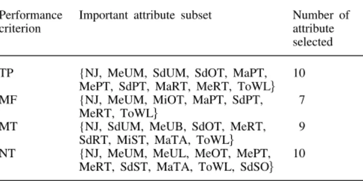
When the values of network weights are generated, we use Eqs (11) and (12) to calculate attribute selection scores to measure important system attributes. The scores of system attributes for each performance criterion are presented in Table 7 and the results of the selected attributes are shown in Table 8.

5.3 Scheduling Knowledge Bases Building and On-line Simulation Verification

To verify whether the selected attributes for FMS system are effective in building scheduling knowledge bases, all of the training examples generated from stage 1 with their important attributes will be retrained to build the new scheduling control mechanism. The results will be compared with individual dis-patching rules and original scheduling knowledge bases from stage 2 for each performance criteria under various system scenarios. The topology and learning rate of each BP network model for building new adaptive scheduling control mech-anisms are presented in Table 9.

To examine the effectiveness of the ASNNAS system in various system scenarios, a series of simulation experiments were conducted. A stream of arriving jobs, each of a 160 000 min simulation run was generated by using a different set of random seeds. The performance of ASNNAS systems was compared with that of NNAS systems and individual dispatching rules using 20 random seeds based on four perform-ance criteria. Table 10 displays the mean and standard deviation (SD) of 20 simulation runs under different scheduling

stra-Table 6. The design parameter of a selected BP network model in attribute selection processes.

Performance Topology Learning rate Root mean square

criterion error of testing

data

TP 30–7–9 0.3 0.0811

MF 30–16–9 0.4 0.0687

MT 30–11–9 0.4 0.0871

Table 7. The attribute selection score for each performance criterion.

System attribute Attribute selection score

TP MF MT NT NJ 0.0726 0.1055 0.0667 0.0826 MeUM 0.0389 0.0362 0.0155 0.0703 SdUM 0.0542 0.0277 0.0488 0.0249 MeUL 0.0218 0.0202 0.0135 0.0357 MeUB 0.0279 0.0249 0.0491 0.0306 MeUA 0.0075 0.0189 0.0230 0.0245 MiOT 0.0186 0.0371 0.0215 0.0325 MaOT 0.0171 0.0249 0.0278 0.0250 MeOT 0.0328 0.0194 0.0210 0.0419 SdOT 0.0399 0.0271 0.0489 0.0146 MiPT 0.0247 0.0309 0.0191 0.0249 MaPT 0.0555 0.0370 0.0319 0.0212 MePT 0.0454 0.0304 0.0238 0.0331 SdPT 0.0492 0.0828 0.0293 0.0286 MiRT 0.0289 0.0270 0.0311 0.0229 MaRT 0.0502 0.0217 0.0228 0.0326 MeRT 0.0479 0.0354 0.1103 0.0579 SdRT 0.0302 0.0220 0.0443 0.0272 MiST 0.0294 0.0267 0.0362 0.0312 MeST 0.0200 0.0239 0.0217 0.0166 SdST 0.0123 0.0243 0.0203 0.0401 MaTA 0.0263 0.0322 0.0399 0.0332 MeTA 0.0280 0.0271 0.0166 0.0249 SdTA 0.0178 0.0200 0.0175 0.0147 MaWL 0.0191 0.0174 0.0226 0.0171 ToWL 0.1141 0.1156 0.0985 0.0756 MeSO 0.0216 0.0198 0.0205 0.0232 SdSO 0.0198 0.0206 0.0276 0.0400 MeTD 0.0161 0.0174 0.0130 0.0202 SdTD 0.0121 0.0260 0.0171 0.0323

Table 8. The results of selected attributes for each performance cri-terion.

Performance Important attribute subset Number of

criterion attribute

selected TP {NJ, MeUM, SdUM, SdOT, MaPT, 10

MePT, SdPT, MaRT, MeRT, ToWL其 MF {NJ, MeUM, MiOT, MaPT, SdPT, 7

MeRT, ToWL其

MT {NJ, SdUM, MeUB, SdOT, MeRT, 9 SdRT, MiST, MaTA, ToWL其

NT {NJ, MeUM, MeUL, MeOT, MePT, 10 MeRT, SdST, MaTA, ToWL, SdSO其

Table 9. The topology of ASNNAS models.

Performance Topology Learning rate Root mean square

criterion error of testing

data

TP 10-12-9 0.3 0.0791

MF 7-9-9 0.4 0.0692

MT 9-8-9 0.3 0.0874

NT 10-16-9 0.4 0.0801

tegies. ASNNAS systems have been shown to be able to achieve better results measured by all the performance criteria owing to their efficiency.

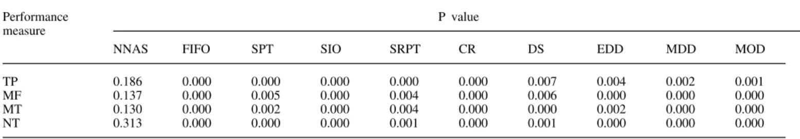
To examine whether the ASNNAS system provides signifi-cant evidence superiority to that provided by the NNAS system and individual dispatching strategies, a paired t-test was perfor-med. A paired t-test does not assume that the mean responses of the dispatching strategies are independent (owing to the use of common random number seeds which are not independent in this study). The null hypothesis is that the mean values of all the scheduling strategies are equal. An overall significance level of 95% was selected for this analysis. The results of the paired t-test are summarised in Table 11.

From the results of the paired t-test, the hypothesis is rejected at the significance level of 95% for all dispatching rules. Therefore, it can be concluded that the performance of the ASNNAS system dominates all of the individual dis-patching rules.

Although no significant discrimination was found between the ASNNAS system and the NNAS system, the performance of the ASNNAS system is shown to be superior to that of the NNAS system measured by each performance criterion.

To further examine the difference between the ASNNAS and NNAS systems, the ability of knowledge bases to select the best dispatching rule at a scheduling control point for each criterion was estimated to the greatest possible accuracy. The

Table 10. A comparison of the mean and SD between ASNNAS and the other scheduling strategy (min).

Scheduling TP MF MT NT

strategy

Mean SD Mean SD Mean SD Mean SD

ASNNAS 5224.00 34.41 1121.08 302.55 739.31 50.18 773.95 81.24 NNAS 5223.85 34.49 1123.11 304.86 768.57 48.54 805.90 83.34 FIFO 5195.35 52.73 2339.86 1126.08 1686.15 148.85 3123.95 123.60 SPT 5214.75 39.56 1146.34 382.21 878.14 69.30 1007.00 101.67 SIO 5206.60 46.13 1509.49 552.78 982.08 77.28 1415.20 121.33 SRPT 5220.50 35.20 1314.07 515.58 875.71 64.17 854.45 84.08 CR 5167.10 61.22 2021.34 775.99 1886.57 75.31 2412.75 120.92 DS 5218.40 39.77 1367.23 609.77 1357.13 155.80 1008.30 119.73 EDD 5204.50 49.19 2110.81 1165.13 1123.80 129.68 2239.25 165.46 MDD 5203.00 49.48 2122.94 1202.03 1262.84 137.67 2231.00 174.38 MOD 5202.65 50.01 2136.97 1197.59 1266.39 143.82 2306.70 177.33

Table 11. A comparison of the paired t-test between ASNNAS and the other dispatching strategy.

Performance P value

measure

NNAS FIFO SPT SIO SRPT CR DS EDD MDD MOD

TP 0.186 0.000 0.000 0.000 0.000 0.000 0.007 0.004 0.002 0.001

MF 0.137 0.000 0.005 0.000 0.004 0.000 0.006 0.000 0.000 0.000

MT 0.130 0.000 0.002 0.000 0.004 0.000 0.000 0.002 0.000 0.000

NT 0.313 0.000 0.000 0.000 0.001 0.000 0.001 0.000 0.000 0.000

greater accuracy implies a better generalisation ability for knowledge bases. Table 12 displays the accuracy of 20 simul-ation runs under two different strategies of scheduling knowl-edge bases. The examination results show that the ASNNAS system can achieve greater accuracy than the NNAS system based on all the performance criteria.

6.

Conclusion

We have developed the ASNNAS system for on-line dis-patching in a dynamic FMS environment. The proposed attri-bute selection algorithm can easily measure the important system attributes that can be used for constructing scheduling knowledge bases. Moreover, less effort is required to build scheduling knowledge bases by using reduced system attributes than by using more system attributes.

The simulation experiment results show that the use of the attribute selection procedure in building scheduling knowledge bases delivers a better production performance than the case in the absence of the attribute selection procedure or the use

Table 12. Accuracy of two scheduling knowledge bases on various performance

TP MF MT NT

ASNNAS 0.7113 0.6953 0.6875 0.6516

NNAS 0.6325 0.6578 0.6315 0.6156

of individual dispatching rules. The results of prediction accu-racy also reveal that scheduling knowledge bases through attribute selection can enhance the generalisation ability based on various performance criteria.

This study did not verify whether this attribute selection algorithm is applicable to other machine learning methods such as decision tree learning so we would like to study this topic in the near future. In addition, how to improve the generalis-ation ability of scheduling knowledge bases corresponding to the continuously shifting environment of product mix is another important issue for further research.

References

1. A. T. Jones and C. R. Mclean, “A proposed hierarchical control architecture for automated manufacturing systems”, Journal of Manufacturing Systems, 5(1), pp. 15–25, 1986.

2. H. Cho and R. A. Wysk, “A robust adaptive scheduler for an intelligent workstation controller”, International Journal of Pro-duction Research, 31(4), pp. 771–789, 1993.

3. N. Ishii and J. J. Talavage, “A mixed dispatching rule approach in FMS scheduling”, International Journal of Flexible Manufacturing Systems, 6, pp. 69–87, 1994.

4. J. Liu and B. L. MacCarthy, “The classification of FMS scheduling problems”, International Journal of Production Research, 34(3), pp. 647–656, 1996.

5. S. C. Park, N. Raman and M. J. Shaw, “Adaptive scheduling in dynamic flexible manufacturing systems: a dynamic rule selection approach”, IEEE Transactions on Robotics and Automation, 13(4), pp. 486–502, 1997.

6. J. H. Blackstone, D. T. Philips Jr and G. L. Hogg, “A state-of-the-art survey of dispatching rules for manufacturing job shop

operations”, International Journal of Production Research, 20(1), pp. 27–45, 1982.

7. K. R. Baker, “Sequencing rules and due-date assignments in a job shop”, Management Science, 30(9), pp. 1093–1104, 1984. 8. M. Montazeri and L. N. Van Wassenhove, “Analysis of scheduling

rules for an FMS”, International Journal Production Research, 28(4), pp. 785–802, 1990.

9. I. Sabuncuoglu, “A study of scheduling rules of flexible manufac-turing systems: a simulation approach”, International Journal Pro-duction Research, 36(2), pp. 527–546, 1998.

10. S. D. Wu and R. A. Wysk, “An application of discrete-event simulation to on-line control and scheduling in flexible manufactur-ing”, International Journal of Production Research, 27(9), pp. 1603–1623. 1989.

11. M. J. Shaw, S. Park and N. Raman, “Intelligent scheduling with machine learning capabilities: the induction of scheduling knowledge”, IIE Transactions, 24(2), pp. 156–168, 1992. 12. Y. Arzi and L. Iaroslavitz, “Operating an FMC by a

decision-tree-based adaptive production control system”, International Journal of Production Research, 38(3), pp. 675–697, 2000.

13. Y. L. Sun and Y. Yih, “An intelligent controller for manufacturing cells”, International Journal of Production Research, 34(8), pp. 2353–2373, 1996.

14. Y. Arzi and L. Iaroslavitz, “Neural network-based adaptive pro-duction control system for flexible manufacturing cell under a random environment”, IIE Transactions, 31, pp. 217–230, 1999. 15. W. Siedlecki and J. Sklansky, “On automatic feature selection”,

International Journal of Pattern Recognition and Artificial Intelli-gence, 2(2), pp. 197–220, 1988.

16. W. Siedlecki and J. Sklansky, “A note on genetic algorithms for large-scale feature selection”, Pattern Recognition Letters, 10, pp. 335–347, 1989.

17. C. C. Chen and Y. Yih, “Identifying attributes for knowledge-based development in dynamic scheduling environments”, Inter-national Journal of Production Research, 34(6), pp. 1739–1755, 1996.

18. C. C. Chen and Y. Yih, “Auto-bias selection for learning-based scheduling systems”, International Journal of Production Research, 37(9), pp. 1987–2002, 1999.

19. D. E. Rumelhart, G. E. Hinton and R. J. Williams, Learning Internal Representations by Error Propagation. Parallel Distributed Processing, MIT Press, Cambridge, MA, 1986.

20. D. W. Patterson, Artificial Neural Networks: Theory and Appli-cations, Prentice–Hall, Singapore, 1996.

21. B. Widrow, R. G. Winter and R. A. Baxter, “Learning phenomena in layered neural networks”, Proceedings of the First IEEE Inter-national Conference on Neural Networks, San Diego, vol. 2, pp. 411–429, 1987.

22. G. D. Garson, “Interpreting neural network connection weights”, AI Expert, pp. 47–51, April 1991.

23. P. M. Wong, T. D. Gedeon and I. J. Taggart, “An improved technique in porosity prediction: a neural network approach”, IEEE Transactions on Geoscience and Remote Sensing, 33(4), pp. 971–980, 1995.

24. SIMPLE⫹⫹, Reference Manual Version 7.0, Stuttgart, AESOP, 2000.

25. NeuralWorks, Professional II Plus Reference Guide, Pittsburgh, PA, NeuralWare, 2000.

Notation

t time at which a decision is to be made

T scheduling period

i job index

j operation index

k machine index (K ⫽ number of machines)

a AGV index (A ⫽ number of AGVs)

l load/unload station index (L ⫽ number of

load/unload station)

p pallet buffer index (P ⫽ number of pallet buffer)

Wk working time percentage on machine k in

simul-ation period

Wa working time percentage on AGV a in simulation

period

Wl working time percentage on load/unload station l in

simulation period

Wp working time percentage on pallet buffer p in

simul-ation period

Pij processing time of the jth operation on job i

Pk

ij processing time of the jth operation on job i in

machine k

Pl

y processing time of the jth operation on job i in

load/unload station l

ARi time at which job i arrived at the system

Di due date of job i

Ci time at which job i is completed and leaves the

system

SJ set of jobs within the system

SF set of finished jobs

SRi set of remaining operations of the job i

兩SJ兩 cardinality of S(t) 兩SF兩 cardinality of F(t)

Fi flow-time of job i (Fi ⫽ Ci ⫺ ARi)

Ti tardiness of job i (Ti⫽ Max(0, Ci ⫺ Di))

SLi slack time of job i (SLi ⫽ Di ⫺ t ⫺

冘