Tools and Algorithms for Protein Structures Comparison with Various Initial Con¯gurations

Tools and Algorithms for Protein Structures

Comparison with Various Initial Configurations

Hong-Shin Chen

Wei-De Jiang

Yaw-Ling Lin

Department of Computer Science and Information Engineering,

Providence University,

200 Chung Chi Road, Shalu, Taichung County, Taiwan 433.

[email protected], [email protected], [email protected]

pro-vide the opportunity to recognize homology that is undetectable by sequence comparison, and it rep-resents a powerful means of discovering functions, yielding direct insight into the molecular mech-anisms. Currently, there are several techniques available in attempting to find the optimal align-ment of shared structural motifs between two pro-teins.

In this paper, we propose algorithms and develop tools for local alignment between two protein struc-tures by means of local adjustment. In our pre-vious work [18], we show that the trigonometric series approximation is appropriate for estimating the good isometric transformations of one struc-ture and aligning it to the other strucstruc-ture. Based on these results, here we propose algorithms to re-fine the given alignment by stepwise finding better alignments of the protein pairings using minimum bipartite matching method on geometric distance space and several other adjustment strategies. The proposed methods are used to improve the given initialized alignment of two structures.

Furthermore, we also propose several prelimi-nary initialization algorithms to examine the ef-fectiveness of the proposed local refinement algo-rithms. We show the effectiveness of the proposed refinement methods and initial algorithm by a set of experiments, which improve several previous re-sults. Furthermore, some of our preliminary result is accessible through the web interface.

∗_{Corresponding author. This work is supported in} part by the National Science Council (NSC 98-2221-E-126-007), Taiwan, Republic of China.

Keywords: structural proteomics, algorithms, structure alignments and comparisons, rmsd, min-imum bipartite matching, secondary structure, combined algorithms.

1

Introduction

Protein structures play critical roles in vital bi-ological functions [10]. With more than 59,000 protein structures determined by the advances in X-ray crystallography and NMR spectroscopy to date, molecular biologists these days proceed in the direction of analyzing and classifying these protein structures in order to discover the struc-tural relationships with protein functions [7].

Detection of proteins with a similar fold can suggest a common ancestor, and often a similar function [6]. Comparison of 3D structures makes it possible to establish distant relationships, even between protein families distinct in terms of se-quence comparison alone. This is why structural alignment of proteins increases our understanding of more distant evolutionary relationships [3, 13]. There have been several methods proposed to compare protein structures and measure the de-gree of structural similarity based on alignment of secondary structure elements as well as alignment of intra and inter-molecular atomic distances. The basic ideas are rapid identification of pair align-ments of secondary structure elealign-ments, clustering them into groups, and scoring the best

substruc-ture alignment. For examples, the VAST

sys-tem [5] is based on continuous distribution of do-mains in the fold space. The FSSP/DALI system

[12] provides two levels of description – a coarse-grained one and one with a fine-coarse-grained resolu-tion. The method, CATH, provides the complete PDB fold classification by domains and links to other sources of information. The two methods, CE and LGscore2 [19] focus on the local geome-try rather than global features such as orientation of secondary structures and overall topology (as in the case of VAST or DALI). VAST has been used to compare all known PDB domains to each other. The results of this computation are in-cluded in NCBI’s Molecular Modelling Database at http://www.ncbi.nlm.nih.gov/Structure/-VAST/vast.html.

Note that there must be an atom-pairing scheme before one can do the structure alignment computation. The first atom of the first selection is compared to the first atom of the second selec-tion, fifth to fifth, and so on. Incorporating with ideas of bipartite matching and 3-parameter iso-metric transformation, Lin et al. [14] proposed methods of using parametric searching strategies with adaptive controls, and demonstrated that more accurate and similar protein structure pair-ings are possible comparing to previous known re-sults like VAST [5] or CE [19].

One of the crucial steps of these algorithms is finding a good isometric transformation, which leads to the best atom-pairing alignment between two proteins. In this paper, we propose algorithms of for efficiently locating more suitable isometric transformations of one structure and aligning it to the other structure. Based upon the periodical property of the parametric settings, we propose parametric searching strategies by approximations with power series and trigonometric series. We show the effectiveness of the proposed parametric searching strategies by a set of experiments, which leads to better alignments of structure pairing in general.

2

Background and Terminology

The main idea of our local refinement algorithm for finding a suitable matching between two sets of points before utilizing the Rmsd procedure to fine-tune the final result is by adjusting the suitable parameter sets by ways of searching the underlying parametric space.

Root mean squared deviation

The smallest root mean squared deviation (rmsd) is a least-squares fitting method for two sequences of points [12]. The idea is to align atom vectors of the two given (molecular) structures, and use the common least averaged squared errors as a mea-surement of differences between these two (paired)

sequences. Formally, let P = hp1, . . . , pni and

Q = hq1, . . . , qni be two sequences of points. We assume that P is translated so that its centroid

(_n1Pn_k=1pk) is at the origin. We also assume that

Q is translated in the same way. For each point

or vector x, let (x)i(i = 1, 2, 3) denote the i-th

(X, Y, Z) coordinate value of x, and kxk denote the length of x. Let

rmsd(P, Q, R, a) = v u u t 1 n n X k=1 kRpk+ a − qkk2,

where R is a rotation matrix and a is a translation vector. Then, the rmsd value d(P, Q) between P

and Q is defined by d(P, Q) = minR,ad(P, Q, R, a).

Schwartz [17] showed that d(P, Q, R, a) is mini-mized when a = 0 and

R = (AtA)12A−1,

where the matrix A = (A_ij) i, j = 1, 2, 3 is given

by Aij = n X k=1 (pk)i(qk)j,

where A12 = B means BB = A , and o denotes

the zero vector. Thus, d(P, Q), R and a can be computed in O(n) time [15].

We use the the McLachlan algorithm [15] as the Rmsd fitting method and write a program in C language to calculate the rmsd between C-α atoms of paired protein backbones.

After locating the appropriate suggested points, the minimum bipartite matching algorithm is used to find the best matching between two sets to de-cide the best matching alignment, which is needed

for the Rmsd procedure. Let P0 = T ◦ P , and Q

being translated to Q0 _{such that the mass}

cen-ter of Q0 _{is located at the origin. We construct a}

weighed graph G = (V, E) with V being labelled

with points of P0 _{and Q}0_{, and each (p, q) in E}

being weighted with the squared Euclidean (3D)

distance; i.e., w(p, q) = kp, qk2. We then solve the

to obtain the best matching of P0 _{and Q}0_{. By the} matched pairing, we perturb and refine the final alignment to obtain a prosbably lower rmsd.

Isometric rotation transformation

According to Euler’s rotation theorem [8], any ro-tation about the origin point can be described by using three angular parameters. The rotation is determined by 3 consecutive rotations with 3

Eu-ler angles (α, β, γ). The first rotation is done by

the angle α around the z-axis, the second is done by the angle β around the x-axis, and the third rotation is done by the angle γ around the z-axis. See [11] for more detailed discussions about the transformation.

Similar to Euler’s rotation transformation, our 3-parameter method (α, β, γ) can be summarized as the following:

• Rotation around z-axis:

Given a unit vector p = (x, y, z)T_{, p is}

trans-formed into p0_{by a rotation around the z-axis}

by angle α. That is, let

p0=   x_yαα zα   = 

 _{− sin απ cos απ 0}cos απ sin απ 0

0 0 1

  · p

Since sin θ = α and thus, cos θ =√1 − α2_.

• Rotation around x-axis:

The vector, p0 = (xα, yα, zα)T, is transformed

into the probe p00_{by a rotation around the}

x-axis by angle β. That is, let

p00=   x_yββ z_β   =   1_{0 cos βπ − sin βπ}0 0 0 sin βπ cos βπ  ·p0

then we will get new coordinate of

(xβ, yβ, zβ)T.

• Rotation around the probe p00_:

The last rotation matrix, Rγ, do the body

rotation around the probe p00_{by angle γ; see}

[11] for related discussions about the trans-formation. That is, let

(x, y, z) = (xβ, yβ, zβ)T. c = cos γπ, s = sin γπ, h = 1 − c. Rγ=   c + x 2_{h xyh − zs xzh + ys} xyh + zs c + y2h yzh − xs xzh − ys yzh + xs c + z2_h  

As a result, we reduce the problem of finding the good rotation matrix to the new problem of finding a good 3-parameter setting. The rotation matrix is thus characterized by just adjusting the 3 uniformly distributed parameters.

Minimum bipartite matching

We use the minimum bipartite matching to find the best matching between two sets of points to de-cide the best matching for the rmsd procedure. We adopted the Munkres [16, 2] algorithm. The public available implementation is written with the Perl language. To improve the efficiency of computa-tion, we implement the Munkres algorithm and write hundreds lines of C Codes.

2.1 Parametric adjustment with

trigono-metric series

In our previous work [18], the trigonometric se-ries estimation method, the three parameters are assumed to be independent. We adjust the three parameters one by one and increase the power of the estimated function. The trigonometric series function is described as the following:

f (θ) = C1+ C2cos πθ + C3sin πθ

+ C4cos 2πθ + C5sin 2πθ

+ C6cos 3πθ + C7sin 3πθ + . . .

+ C_2kcos kπθ + C_2k+1sin kπθ.

(1)

where f (θ) denote the corresponding value of

rmsd with respect of one of the three parameters,

(α, β, γ). The k usually reflects the numbers of local maximal points in the approximated curve.

2.2 VAST

It performs all-on-all structure comparisons using the VAST algorithm. VAST is based on aligning secondary structure elements using an algorithm from the field of graph theory .The

output is a neighbors D list. It also contains

the complete PDB representative structure comparison structure alignments and a structure superposition tool. The search space for alter-native secondary structure elements depends on

the length of proteins. All pairs of secondary

structure elements (one from each structure) that have the same type are represented as nodes of a graph. Two nodes are connected by an edge

if the distance and angle between the corre-sponding pairs of secondary structure elements from the two proteins are within some threshold. The graph therefore represents correspondences between pairs of secondary structure elements that have the same type, relative orientation, and connectivity. This correspondence graph is then searched to find the maximal subgraph such that every node in the subgraph is connected to every other node in the subgraph and is not contained in any larger subgraph with this property. This is referred to as clique detection in graph theory and is basis of finding the initial

secondary structure alignment. VAST extends

this initial alignment to a residue level alignment

using a Gibbs sampling [4] technique. VAST

places considerable emphasis on defining the statistical significance of an alignment. For each pairwise alignment, the algorithm computes an alignment score as well as a P-value for the best substructure superposition. The P-value assigned to the alignment is calculated as the probability that its score would be seen by chance in drawing secondary structure pairs at random from the database multiplied by the number of possible alternative substructure alignments for the given

pair of structures. The program only reports

alignments that yield a P-value less than 0.05. A P-value of 0.05 indicates that VAST expects to find an alignment with the same degree of similar-ity by chance in 5% of all pair-wise comparisons. VAST uses a threshold of 0.05 to limit the noise in the hit lists, thus allowing repeated iterations of double neighboring in Entrez . VAST has been used to compare all known PDB domains to each other. The results of this computation are in-cluded in NCBI’s Molecular Modeling Database at http://www.ncbi.nlm.nih.gov/Structure/VAST/ vast.html.

2.3 Initialization by Main Vector Method

The initial method, such as VAST and CE, sup-ports the trigonometric series estimation method to improve the rmsd value. A better initial align-ment is very important for the trigonometric se-ries estimation method to adjust a better result. Therefore, we try to develop a initial method ac-cording to the shape of protein structure. The main vector method is to find a main vector about protein structure in 3-dimension and a second main vector in 2-dimension. We apply the

in-ner and outer product to find the rotation and vertical vector. Let x, y be two vectors and θ be the included angle of x and y. We can have

θ = cos−1 hx·yi

kxk·kyk, then we use the outer product

to find the vertical vector, v, which is defined as v = x × y, then we use θ and v to rotate the protein structure. The algorithm is shown in Fig-ure ??. In this algorithm, we have a first main vector and a second main vector. If we assume a, b to stand for the two points of first main vector and c, d to to stand for another. There are totally four possible combinations for them, (−ab,→ −cd), (→ −ba,→ cd), (−→ −ab,→ −dc), (→ −ba,→ −dc). We choose→ the minimum rmsd of them to be the initial rota-tion. Besides the main vector method, we also use a random initial rotation to execute the trigono-metric series estimation method. The experimen-tal results of those two different settings are dis-cussed in next section.

2.4 Initialization by segment alignment

Comparing to the more sophisticated methods like CE or VAST, the main-vector initialization position [18] does have the advantage of saving valuable computation resources. Yet the initial orientation found by the main-vector method does not produce satisfactory final orientation even af-ter the fine-tune procedures. The idea here is try-ing to find more suitable starttry-ing positions and still conserve enough computation time for later adjustment. Since the protein structure is just a chain sequence of atoms, we can subdivide the sequence and use the subsequence matching infor-mation to find the better alignment. Thus, the atom chains of a structure is divided into several (consecutive) segments.

Given a list of (consecutive) atoms obtained from the PDB file [1], one way of dividing pro-tein chains of a structure is by using the secondary structural information of the given protein. That is, for the secondary structural partition method, the segments of structures is determined by parti-tion the protein sequence by the secondary struc-tural information of the given protein. Another possible division scheme is obtained by slicing a fixed number of atoms of the given protein. Thus, for the fixed number partition method, the seg-ments of structures is determined by partition the protein sequence by a fixed number of atoms of the given protein.

segment alignment uses the standard dynamic

pro-gramming technique to obtain feasible pairings be-tween segments by maintaining a suitable score ta-ble. The dynamic programming evaluation func-tion is described as the following:

score(s, λ) = U mp · | s | score(λ, t) = U mp · | t | score(sx, ty) = min        Rmsd(L(s, t) ◦ Match(x, y)) · ` + U mp · (| sx | + | ty | −2`) score(sx, t) + U mp · | y | score(s, ty) + U mp · | x |

here λ denotes the empty list; s and t are two pre-fix segment lists. L(s, t) is the alignment between

segment lists s and y, and nL denotes the number

of atoms in L; ` =| L(s, t) ◦ Match(x, y) |. The recurrence relation for evaluating the value

score relies on three possible alignments between sx and ty. Here s and t are two prefix segment lists, and x and y are the two currently (last)

con-sidered segments. The first alignment, L is the pairing list from L(s, t) merging with Match(x, y) which stands for the match between segment x

y. Since Rmsd() returns the average

precalcu-lated rmsd value, the number is multiplied by the number of matched pairs `. However, if one can not find any match for an atom, a given punish-ment constant, U mp, must be added to encour-age most atom be aligned with some atoms on the other sequence. Another possibility is the case of

score(sx, t); in that case, the segment y is not able

to match with segment on the other list. Thus we need to add in the punishment values for all atoms of the y segment. The case of score(s, ty) is also treated similarly.

3

Methodology

In this section, first we introduce the motivation about why we want to use the local refinement algorithm to find the better list between two pro-teins. Secondly, we show the initial algorithm ac-cording to the structure of protein. The detail experimental result is showed in next section.

3.1 Motivation

In our previous works, the trigonometric series estimation method is used to find a better posi-tion in protein structure comparison. Let P A and

P B denote two protein structures. The proposed

method partitions atoms of a given protein by a fixed length, forming a list of segments. By us-ing the dynamic programmus-ing technique, the al-gorithm aligns segments of P A to segments of P B to obtain the initial configuration; then the algo-rithm proceeds with trigonometric series estima-tion method to further improve the control param-eters of the 3D isometric transformation in order to further refine the final alignment list. We also develop another initial methods, main vector as an substitute for the well-known methods, such as the VAST and CE. In the following we introduce the segment alignment initialization algorithm.

3.2 Initialization by New Segment

Align-ment

Let A = {a1, a2, a3. . . , ai} and B =

{b1, b2, b3. . . , bi} are two list of 3D coordinates

of point, and C = {c1, c2, c3. . . , ci} are center of

gravity of A and B. The p is not match point with

segment. W (p) = min{d(p, Ci)} is weight of point

p. score(s, λ) = U mp · | s | score(λ, t) = U mp · | t | score(sx, ty) = min        Rmsd(L(s, t) ◦ Match(x, y)) · `

+P_{p∈sx∪ty\L}0min_q∈Center(L0₎{d(p, q)})

score(sx, t) +P_p∈ymin_{q∈Center(L)}{d(p, q)} score(s, ty) +P_p∈xmin_{q∈Center(L)}{d(p, q)} L(s, t) is the alignment between segment lists s

and y, and nL denotes the number of atoms in L;

` =| L(s, t) ◦ Match(x, y) |.

3.3 Parametric adjustment with

trigono-metric series

By incorporating with the two key concepts, parameterized-rotation as well as bipartite match-ing, the main algorithm can compare paired pro-tein structures once given a reasonable good initial setting of the 3 parameters. Since the best para-metric settings can be very difficult to locate, our previous methods concentrate on using random-ized perturbation method in searching sufficiently large number of parametric probes over the pa-rameter spaces and let each probe searching its own proximity in a randomized greedy manner. It is shown that the underlying corresponding rmsd

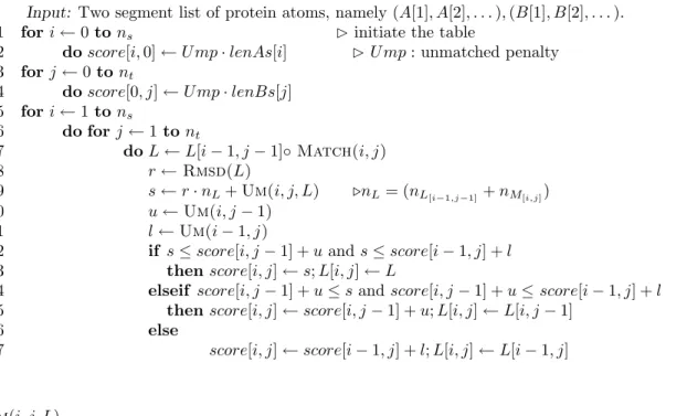
Seg-Alig ¤Segment Alignment algorithm

Input: Two segment list of protein atoms, namely (A[1], A[2], . . . ), (B[1], B[2], . . . ). 1 for i ← 0 to ns ¤ initiate the table

2 do score[i, 0] ← U mp · lenAs[i] ¤ U mp : unmatched penalty 3 for j ← 0 to nt 4 do score[0, j] ← U mp · lenBs[j] 5 for i ← 1 to ns 6 do for j ← 1 to nt 7 do L ← L[i − 1, j − 1]◦ Match(i, j) 8 r ← Rmsd(L)

9 s ← r · nL+ Um(i, j, L) .nL= (nL[i−1,j−1]+ nM[i,j])

10 u ← Um(i, j − 1)

11 l ← Um(i − 1, j)

12 if s ≤ score[i, j − 1] + u and s ≤ score[i − 1, j] + l 13 then score[i, j] ← s; L[i, j] ← L

14 elseif score[i, j − 1] + u ≤ s and score[i, j − 1] + u ≤ score[i − 1, j] + l 15 then score[i, j] ← score[i, j − 1] + u; L[i, j] ← L[i, j − 1]

16 else

17 score[i, j] ← score[i − 1, j] + l; L[i, j] ← L[i − 1, j]

Um(i, j, L)

Input: The L is the pairing list. 1 D ← A[1, . . . , i] ∪ B[1, . . . , j] − L 2 C ←Cofg(L)

3 p ←Ump(C, D) 4 return p

Cofg(L) return the center of gravity of L list pairs.

Ump(C, D) return the weight of minimum distance sum of center of gravity C and dropped point set D.

values associated with the parametric sets are re-lated to each other in periodical and continuous manner; thus seeking reasonable approximation of the underlying rmsd values distributions is possi-ble by some suitapossi-ble mathematical models, espe-cially by trigonometric series [14].

Here we further improve our previous results and propose an algorithm that further exploit more phases of the trigonometric series estimation methodology. As shown in Figure 2, the algorithm consists of 3 phases. The algorithm first spreads g

guessing points uniformly over the underlying

nor-malized parameter space ranged (−0.5, +0.5); sec-ondly, the algorithm proceeds with h estimation

points by trigonometric series estimation function.

These g + h phases are repeated over all three pa-rameters searching spaces. Finally, these paramet-ric searching processes are performed by exactly

f rounds. Each parametric searching process

usu-ally alternates one of these three parameters space; once the isometric transformation is set, the atoms of one protein are transformed and matched (by bipartite matching method) with the other pro-tein. Thus, there are totally 3f (g + h) MBM op-erations performed for the structure alignment re-finement algorithm.

4

Experimental

Results

And

Web System

In this section, we introduce the target of exper-imental data set first. Then we show the difference with dividing protein chains of a structure depends on the different secondary structures of the given protein. Finally, we show the Web enable user can use our system through the network.

4.1 Data Set

We choose the PDB for our experimental sam-ple source, and we randomly pick 14,400 protein structures in the PDB database as our experi-mental subjects by the uniform distribution sam-pling out of totally 59,618 protein structures as of 2009. For each chosen protein structures we ran-domly choose one structure alignments listed on the database of VAST as the tested targets. We use the term, P , to stand for one of the 14,400 randomly picked protein structures, and we use Q to stand for one of the neighbors of each P . Note that P and Q include all un-aligned and aligned

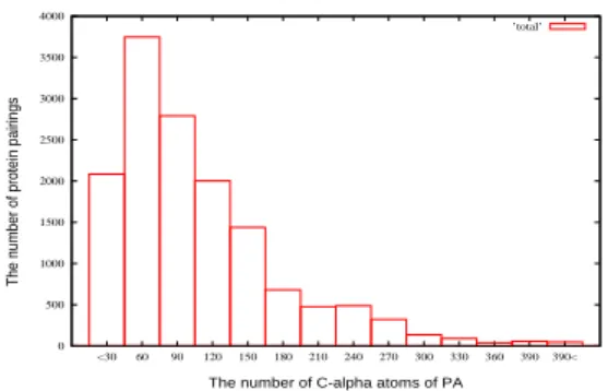
atoms. We use the term, P A, to stand for the aligned atoms of P by VAST, and we use P B to stand for one of the neighbors of each PA. Totally, there have 14,400 protein pairings can test by our previous experiment. The distribution of them is shown in Figure 3. In this paper we randomly pick 1,000 protein pairings from 14,400 protein pairings to test our experiment.

0 500 1000 1500 2000 2500 3000 3500 4000 <30 60 90 120 150 180 210 240 270 300 330 360 390390<

The number of protein pairings

The number of C-alpha atoms of PA

’total’

Figure 3: The distribution of the 14,400 ran-domly picked protein structures in PDB and their one neighbor structures. The total num-ber of protein pairs is 14,400.

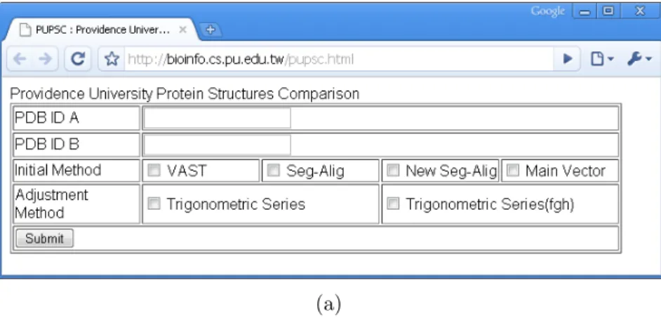
4.2 Web System

We make a web system, the Providence

University Protein Structure Comparison Web System, for users who are interested

in our structures comparison system at

http://bioinfo.cs.pu.edu.tw/pupsc.html. The user of our web service usually provides

two protein PDB IDs. We provide three

ini-tial methods, and two parametric adjustment methods. Our web system searches and obtains the corresponding PDB data from the Protein data bank database [1] and perform the desired protein structure alignment/comparison using the chosen set of algorithms. To avoid the time delay, our web service provides user access keys for user to check the result later. Users can come back and check the comparison result after the computation is completed by the system servers; parts of our web entry interface are shown in Figure 7.

5

Concluding Remarks

In this paper, we propose algorithms to improve the rmsd value between a protein structure pair

Struc-Align(P, Q, αI, βI, γI, p)

Input: Two set of 3D coordinates of points P = {p1, p2, . . . , pn} and Q = {q1, q2, . . . , qm} ; n < m. The αI , βI and γI are real numbers that are between -0.5 to 0.5.

¤ These inputs control the initial position of 3 parameters box and affect the explored area. ¤ p is the vector (x, y, z)T_{, explained in section 2.4.}

Output: (s, α, β, γ) is a sufficiently low Rmsd s and (α, β, γ). ¤ (α, β, γ) is the best position of 3 parameters box. Global : f, g, h, θmax.

The threshold F ,G,H are integer numbers. ¤ F is number of uniformly spreading probes. ¤ G is number of adaptively estimating probes. ¤ H is number of adjustment rounds.

θmax is real numbers of control the parametric perturbation variances between -0.5 to 0.5. 1 (α, β, γ) ← (α∗_{, β}∗_{, γ}∗_{) ← (α}

I, βI, γI)

2 Q0 _{← Trans(Q,Rot-m(α, β, γ, p)) ¤ Q}0 _{is a temp array of atoms set of protein.} 3 L ← Mbm(P, Q0_{) ; (R, a) ←Ms-Fit(L, P, Q}0_{) ; s}∗_{←Rmsd(P, Q}0_{, R, a)}

4 for t ← 1 to h

5 do for i ← 1 to 3

6 do (θ[1], θ[2], θ[3]) ← (α, β, γ) ¤Reset parameters θ[i]s. 7 S[1] ← s ; U [1] ← θ[i]

8 for k ← 2 to f + 1 ¤Spreading f probes. 9 do θ[i] ← U [k] ←Rand(−θmax, θmax) 10 Q0_{← Trans(Q,Rot-m(θ[1], θ[2], θ[3], p))}

11 L ← Mbm(P, Q0_{) ; (R, a) ←Ms-Fit(L, P, Q}0_{) ; s ← S[k] ←Rmsd(P, Q}0_{, R, a)} ¤ S is an array to save the rmsd.

12 if s ≤ s∗

13 then s∗_{← s ; (α, β, γ) ← (α}∗_{, β}∗_{, γ}∗_{) ← (θ[1], θ[2], θ[3]) ;}

14 z ← f + 1

15 for j ← 1 to g/2 ¤Estimating g probes.

16 do z ← z + 1 17 θ[i] ← U [z] ←Lowest(z, U, S) 18 Q0_{← Trans(Q,Rot-m(θ[1], θ[2], θ[3], p))} 19 L ← Mbm(P, Q0_{) ; (R, a) ←Ms-Fit(L, P, Q}0_{) ; S[z] ←Rmsd(P, Q}0_{, R, a)} 20 if s ≤ s∗ 21 then s∗_{← s ; (α, β, γ) ← (α}∗_{, β}∗_{, γ}∗_{) ← (θ[1], θ[2], θ[3]) ;} 22 z ← z + 1 23 (U0_{, S}0_{) ←DelMin(U, S)} 24 θ[i] ← U [z] ←Lowest(z, U0_{, S}0₎ 25 Q0_{← Trans(Q,Rot-m(θ[1], θ[2], θ[3], p))} 26 L ← Mbm(P, Q0_{) ; (R, a) ←Ms-Fit(L, P, Q}0_{) ; S[z] ←Rmsd(P, Q}0_{, R, a)} 27 if s ≤ s∗ 28 then s∗_{← s ; (α, β, γ) ← (α}∗_{, β}∗_{, γ}∗_{) ← (θ[1], θ[2], θ[3]) ;} 29 return (s∗_{, α}∗_{, β}∗_{, γ}∗₎

Mbm(P, Q) returns the minimum bipartite matching of two point sets P and Q.

DelMin(U, S) returns two arrays U0_{, S}0 _{such that the largest element in S, and it’s corresponding element.} Lowest(z, U, S).

Input: The z is number of probes. The U is an array of angles. The S is an array of rmsd0_s. Output: (θ∗₎

1 for i ← 1 to z 2 M atrix[i][1] ← 1 3 for j ← 1 to z−1₂

4 M atrix[i][2j] ← cos(jπU [j]) ; M atrix[i][2j + 1] ← sin(jπU [j])

5 C ←GaussElim(M atrix, S) ¤The estimated function is f (θ) = C[1] + C[2]cosπθ + C[3]sinπθ + . . . 6 θ∗_{← arg min}

−0.5≤θ≤0.5f (θ) ¤f (θ) is the estimated function. 7 return (θ∗₎

Rand(a, b) is a random function returning a real number uniformly distributed between a and b. Trans(A, R).

Input: A is an array of 3D points with size n. R is the rotation matrix.

Output: An array of 3D points,B. 1 for i ← 1 to n do

2 B[i] ← R · A[i] ¤ B is the array containing the transformed n points. 3 return B

Figure 2: Aligning two sets of atoms with low rmsd by pairing points according to the minimum bipartite matching measurement .

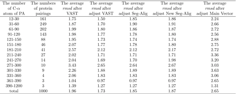
The number The numbers The average The average The average The average The average of C-α of protein rmsd after rmsd after rmsd after rmsd after rmsd after atom of PA pairings VAST adjust VAST adjust Seg-Alig adjust New Seg-Alig adjust Main Vector

12-30 161 1.75 1.50 1.85 1.86 2.24 31-60 249 1.87 1.70 1.90 1.91 2.66 61-90 202 1.99 1.80 1.86 1.87 2.72 91-120 143 1.98 1.77 1.78 1.80 2.56 121-150 88 1.95 1.73 1.74 1.74 2.88 151-180 46 2.07 1.77 1.78 1.80 2.75 181-210 41 2.57 2.12 2.12 2.17 2.72 211-240 27 2.02 1.71 1.71 1.71 3.36 241-270 14 2.04 1.69 1.70 1.98 3.20 271-300 10 3.43 2.65 2.64 2.67 3.03 301-330 9 2.26 1.88 1.89 1.89 3.63 331-360 4 2.06 1.83 1.83 1.83 3.06 361-390 3 1.04 0.97 0.97 0.97 2.65 390-1200 3 1.39 1.27 1.27 1.27 1.31 total 1000 1.96 1.73 1.85 1.87 2.65

Table 1: The result is to execute the algorithm of three initial method and VAST. This table show initial method rmsd and after adjustment rmsd. The unit of rmsd values is measured by Angstrom(˚A = 10−8_cm.).

1.0000 2.0000 3.0000 4.0000 5.0000 6.0000 7.0000 8.0000 9.0000 <30 60 90 120 150 180 210 240 270 300 330 360 390 390< Averaged rmsd

The number of C-alpha atoms of PA

’OV’ ’OS’ ’OT’ ’OM’ (a) 0.5000 1.0000 1.5000 2.0000 2.5000 3.0000 3.5000 4.0000 <30 60 90 120 150 180 210 240 270 300 330 360 390 390< Averaged rmsd

The number of C-alpha atoms of PA

’OV’ ’AV’ ’AS’ ’AT’ ’AM’ (b)

Figure 4:

The initial The average The average The average

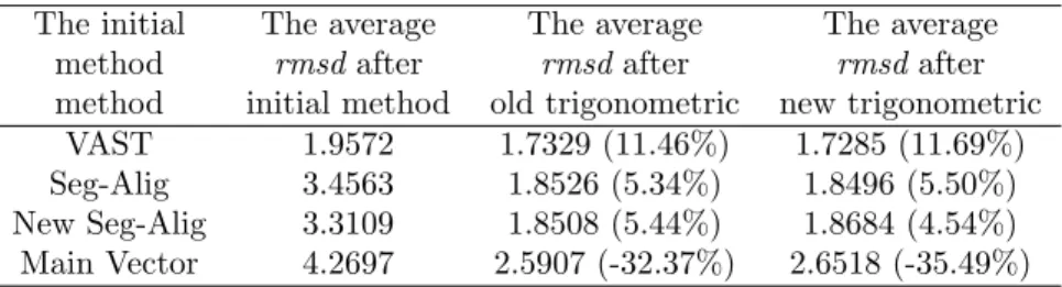
method rmsd after rmsd after rmsd after

method initial method old trigonometric new trigonometric

VAST 1.9572 1.7329 (11.46%) 1.7285 (11.69%)

Seg-Alig 3.4563 1.8526 (5.34%) 1.8496 (5.50%)

New Seg-Alig 3.3109 1.8508 (5.44%) 1.8684 (4.54%)

Main Vector 4.2697 2.5907 (-32.37%) 2.6518 (-35.49%)

Table 2: The result is to execute the algorithm of trigonometric series with initial alignment of

VAST, Seg-Alig, New Seg-Alig and Main vector. These percentages are express improvement of

original Vast.

0.5000 1.0000 1.5000 2.0000 2.5000 3.0000 3.5000 4.0000 4.5000 <30 60 90 120 150 180 210 240 270 300 330 360 390 390< Averaged rmsd

The number of C-alpha atoms of PA

’OV’ ’OS’ ’AS’ (a) 0.5000 1.0000 1.5000 2.0000 2.5000 3.0000 3.5000 4.0000 4.5000 <30 60 90 120 150 180 210 240 270 300 330 360 390 390< Averaged rmsd

The number of C-alpha atoms of PA

’OV’ ’OT’ ’AT’

(b)

Figure 5:

(a)

Figure 7: The web window of input and user menu. User submits can get a access key. After the

system obtain all analyzed results, user can get the result later on through the use of access key.

1.0000 2.0000 3.0000 4.0000 5.0000 6.0000 7.0000 8.0000 9.0000 <30 60 90 120 150 180 210 240 270 300 330 360 390 390< Averaged rmsd

The number of C-alpha atoms of PA

’OV’ ’OM’ ’AM’

Figure 6:

by finding better alignment list. A set of exper-iments is designed to test the parameters; these adjusted parameters are set to perform the ex-periments over over a thousand of protein pairs, which are uniformly random sampled from the PDB database. As the results shown that our methods improve the alignment computed by the VAST by an averaged improvement ratios about 11%. The results demonstrate that the method of using 3D Euclidean distance minimum bipar-tite matching with trigonometric series estimated parametric searching scheme indeed improves ex-isted known system like the VAST. It remains in-teresting to further explore the underlying best suited parameters for our method.

The experiments show that a good initial rota-tion is very important before the parametric ad-justment. The idea of our segment alignment

ini-tial setting methods is to slice a fixed number of atoms and by matching segments of two struc-tures using the dynamic programming technique; the proposed segment alignment method does ob-tain feasible starting configurations. It is shown that, by further incorporated with our proposed trigonometric series estimation method, the com-bined method performs better than the original VAST method by an averaged improvement ratios about 5%. Furthermore, some of our preliminary result is accessible through the our web interface to provide molecular biologists and other bioinfor-matic researchers the use of our service.

Finally, since the structure comparison prob-lem, like many scientific computation/simulation problem, is very time-consuming under cases of large structures and large number of paired struc-tures, it is desirable to implement the system un-der massive parallel machines cluster, e.g., the grid-environment, to increase the throughput of the system.

References

[1] H. M. Berman, J. Westbrook, Z. Feng, G. Gilliland, T. N. Bhat, H. Weissig, I. N. Shindyalov, and P. E. Bourne. The protein data bank. Nucleic Acids Research, 28:235–242, 2000. [2] F. Bourgeois and J. C. Lassalle. An extension of

the munkres algorithm for the assignment prob-lem to rectangular matrices. In Communications of the ACM, volume 14, pages 802 – 804, New York, NY, 1971. USA.

[3] J. M. Bujnicki. Phylogeny of the restriction endonuclease-like superfamily inferred from com-parison of protein structures. J Mol Evol., 50:38– 44, 2000.

[4] G. Casella and I. G. Edward. Explaining the gibbs sampler. The American Statistician, 46:167–174, 1992.

[5] S. Cristobal, A. Zemla, D. Fischer, L. Rychlewski, and A. Elofsson. A study of quality measures for protein threading models. BMC Bioinformatics, 2:5, 2001.

[6] S. Dietmann and L. Holm. Identification of ho-mology in protein structure classification. Nature Struct. Biol., 8:953–957, 2001.

[7] N. Echols, D. Milburn, , and M. Gerstein. Mol-movdb:analysis and visualization of conforma-tional change and structural flexibility. Nucleic Acids Res., 31:478V482, 2003.

[8] L. Euler. Formulae generales pro trandlatione quacunque corporum rigidorum. Novi Acad. Sci. Petrop., 20:189–207, 1775.

[9] Z. Galil. Efficient algorithms for finding maximum matching in graphs. ACM Computing Surveys, 18:1:23–38, 1986.

[10] M. Gerstein, R. Jansen, T. Johnson, J. Tsai, and W. Krebs. Motions in a database framework: from structure to sequence. Rigidity Theory and Appli-cations, pages 401–442 (ed. M F Thorpe and P M Duxbury, Kluwer Academic/Plenum Publishers), 1999.

[11] A. Gray. A treatise on gyrostatics and rotational motion. MacMillan,London, 1918.

[12] L. Holm and C. Sander. Touring protein fold space with DALI/FSSP. Nucleic Acids Res., 26:316– 319, 1998.

[13] M. S. Johnson, M. J. Sutcliffe, and T. L. Blun-dell. Molecular anatomy: Phyletic relationships derived from three-dimensional structures of pro-teins. J Mol Evol., 30:43–59, 1990.

[14] Y. L. Lin and S. P. Huang. Tools and algo-rithms for refined comparison of protein struc-tures. In The 6th WSEAS International Confer-ence on Microelectronics, Nanoelectronics, Opto-electronics (MINO ’07), Istanbul, Turkey, 2007. [15] A. D. McLachlan. Rapid comparison of protein

structures. Acta Cryst, A38:871–873, 1982. [16] J. Munkres. Algorithms for the assignment and

transportation problems. Journal of the Society for Industrial and Applied Mathematics, 5:32–38, 1957.

[17] J. T. Schwartz and M. Sharir. Identification of partially obscured objects in two and three dimen-sions by matching noisy characteristic curves. Int. J. Robotics Research, 6:29–44, 1987.

[18] H. S. Shin, Y. L. Lin, and W. D. Jiang. Pro-tein structures alignment algorithms by paramet-ric searching with trigonometparamet-ric series. In Pro-ceedings of the 25th Workshop on Combinatorial Mathematics and Computation Theory, pages 44– 54, Hsinchu, Taiwan, 2008.

[19] I. N. Shindyalov and P. E. Bourne. Protein struc-ture alignment by incremental combinatorial ex-tension (CE) of the optimal path. Protein Eng., 11:739–747, 1998.