Network Dimensioning Problems of Applying
Achievement Functions
Chia-Hung Wang
∗Hsing Luh
†Department of Mathematical Sciences, National Chengchi University, Wen-Shan, Taipei 11623, Taiwan
Abstract In this paper, we focus on approaches in network dimensioning where it allocates band-widths and attempts to provide a proportionally fair treatment of all the competing classes. We will show that an achievement function can map different criteria onto a normalized scale subject to vari-ous utilities. The achievement function can be coped with the Ordered Weighted Averaging method. Moreover, it may be interpreted as a measure of QoS on All-IP networks. Using the achievement function, one can find a Pareto optimal allocation of bandwidths on the network under the available budget, which provides the so-called proportional fairness to each class. Consequently, this results in the similar satisfaction level to every connection in all classes.
Keywords multiple criteria optimization; achievement function; proportional fairness
1 Introduction
Taking a single global Internet Protocol (IP) based networks to carry all types of services, telecommunication is moving toward a converged network to replace the traditional separated packet switched and circuit switched networks [17]. This revolutionary converged All-IP networks not only reduces network deployment and management costs, but also offers a great deal of opportunity to introduce various new services that are not possible on the traditional separated networks.
The idea of a single shared physical network that will support multiple heteroge-neous applications with different traffic characteristics and different Quality of Ser-vice (QoS) requirements, is widely regarded as a way to meet the telecommunication challenges of the future [3], [19]. Packet-switched networks have been proposed to offer the QoS guarantees in integrated-services networks because individual packets may exhibit a significant variation in network service quality.
Packet switched networks suffer three major quality problems in offering time-sensitive services: long delay time, jitter, packet loss. The Universal Mobile Telecom-munications System (UMTS) offers teleservices (like speech or SMS) and bearer ser-vices which provide the capability for information transfer between access points. It
∗E-mail: [email protected]
†E-mail: [email protected]
is possible to negotiate and renegotiate the characteristics of a bearer service at con-nection establishment or during ongoing concon-nection. Bearer services have different QoS parameters such as maximum transfer delay, delay variation and bit error rate. Thus, UMTS network services have different QoS classes for four types of traffic:
1. Conversational class (voice, video telephony, video gaming) 2. Streaming class (multimedia, video on demand, webcast)
3. Interactive class (web browsing, network gaming, database access) 4. Background class (email, SMS, downloading)
UMTS [17] has specified four different traffic classes according to their QoS requirements for different applications as shown in Table 1. An UMTS network consists of three interacting domains; Core Network (CN), UMTS Terrestrial Radio Access Network (UTRAN) and User Equipment (UE). The main function of the core network is to provide switching, routing and transit for user traffic. A core network also contains the databases and network management functions. The basic Core Network architecture for UMTS is based on GSM network with GPRS. UMTS uses channels with a fixed bandwidth of 5 Mbps, which is transmitted from a base station to all mobile stations [17]. Each station transmits its information using Code Division Multiple Access (CDMA). The available bandwidth can be divided between the users according to their needs. Therefore, a problem of network dimensioning with elastic traffic [11] requires to allocate bandwidth to maximize flows fairly.
Table 1: The Characteristics of UMTS Service Classes
Traffic Classes Sensitivity to Jitter Sensitivity to Delay Sensitivity to Packet Loss
Conversational high high low
Streaming high high low
Interactive class low low high
Background class very low low high
Fair resource allocation problems are concerned with the allocation of limited bandwidth among competing activities so as to achieve the best overall performances of the system but providing fair treatment of all the competitors [8]. We introduce the methodology that allow the decision maker to explore a set of solutions that could satisfy users’ preferences with respect to throughput and fairness (see [4], [5], [11], [12]). The formulation and analysis is carried out in a general utility-maximizing framework. Assume there are m classes in different QoS requirements. In this work, we will adopt the approach called proportional fairness (see [4], [5], [12]) to max-imize the sum of logarithms of the bandwidthθifor each class i, i = 1, . . . , m. The optimization model of the Proportional Fairness method takes the following form:
max m
∑
i=1log(θi) (1)
Different users have different objectives for the network QoS. There are a num-ber of characteristics that qualify QoS [20], including minimum queue delay,
mini-mum delay variations, maximini-mum capacity of consistent data throughput, etc. Multi-ple criteria decision methods are applied in some decision models to aggregate differ-ent criteria measuremdiffer-ents and subjective preference information from the decision-makers (DMs). A more straightforward technique to represent the DMs’ preferences in a decision model is through goals or reference points where the DMs can specify aspiration levels, i.e., desirable or preferable values for each criterion.
In a multiple criteria decision-making situation we often search for Pareto opti-mal solutions. In a typical multiple criteria optimization of realistic size, especially one with more than two objectives, the range of efficient solutions can be enormous. One scheme for dealing with multiple criteria models that permits more balanced handling of the objectives is simply to combine them in a weighted sum. Multiple objective functions can be combined into a single composite one by summing objec-tives with positive weights on maximizing and negative weights on minimizing [15]. Signs orient all objectives in the same direction, and weights reflect their relative im-portance. If a single weighted-sum objective model derived from a multiple-objective optimization produces an optimal solution, the solution is undominated by any other one; simply we call it a Pareto optimal solution of the multiple-objective model. In this work, we use the method of weighted sums to solve (1). When compared to weights, reference points provide a more direct way for the DMs to express their desires and, thus, to affect the solution.
In short, we deal with the problem of dimensioning bandwidth for elastic data applications in packet-switched communication networks, which can be considered as a multiple-objective optimization model. Users’ satisfaction is summarized by means of their achievement functions where each user is allowed to request more than one type of service. The objective of the optimization problem is to determine the amount of required bandwidth for each class to maximize the users’ satisfaction with a proper aggregate utility function. In this regard, we will focus on the following subjects:
i) how to construct the achievement functions involving utility functions; ii) how to transform the different criterion measurement onto a normalized scale; iii) how to allocate budgets with proportional fairness on UMTS networks.
The remaining parts of this paper are organized as follows. In the next sec-tion we introduce the network dimensioning problems where we construct the utility functions function to transform the different measurements onto a normalized scale. A numerical example is given in Section 3. Finally, in Section 4, we remark on summaries of this study.
2 Fair bandwidth allocation on network dimensioning
problems
Consider a core network topology G = (V, E), where V and E denote the set of nodes and the set of links in the network respectively. Given the total budget B and the maximal possible capacity of each link Ue, the objective is to allocate optimal
bandwidth for all connections subject to QoS requirements bi. Suppose there are m different classes which have their own QoS requirement. In each class, every connection is allocated the same bandwidth and it has the same QoS requirement. Suppose each connection is delivered between the same source and destination in this (core) network. Under a limited available budget, we want to allocate the bandwidth xein order to provide each class with maximal possible QoS.
2.1 Network constraints
Denote by Si a set of connections in class i. Suppose there is the number of
connections in Siis Ki, i.e., |Si| = Ki. Given the marginal costκeof bandwidths for each link e ∈ E, it shall allocate the bandwidths in order to provide each class with
maximal possible QoS. First, let xeandθi be the bandwidth allocated to the link e
and the connection j of class i respectively. Then these decision variables must be nonnegative:
xe≥ 0, ∀ e ∈ E (2)
θi≥ 0, ∀ j ∈ Si, for i = 1, . . . , m. (3)
Furthermore, it requires the following constraints on the network:
∑
e∈E
κexe= B (4)
and
xe≤ Ue, ∀e ∈ E. (5)
In each class i, every connection takes the same bandwidth and has the same bandwidth requirement and it producesθi,1=θi,2= · · · =θi,Ki. Letθi(=θi,1=θi,2=
· · · =θi,Ki) be the bandwidth allocated to each connection of class i. Thus, the
con-straint follows
θi≥ bi. (6)
Next, for each connection j of class i, denote by pj the routing path from the
source o to destination d. To determine whether link e is chosen we define the binary decision variable χi j(e) = ½ 1 if link e ∈ pj 0 if link e /∈ pj. (7)
Thus, it yields the following constraint:
∑
i
∑
j χij(e)θi= xe, ∀ e ∈ E. (8)
Moreover, for each class i, it has θi·
∑
e κeχi
where ciis a budget allocated to each connection of class i. Then, it gives
∑
i
(Ki· ci+πi) = B, (10)
whereπi is the reserved budget for each class i. Let Eo ⊆ E be the set of links
connected with the source node o, then we have
∑
e∈Eo
χi
j(e) = 1, ∀ i, j. (11)
Let Ed⊆ E be the set of links connected with the destination node d, then we have
∑
e∈Ed
χi
j(e) = 1, ∀ i, j. (12)
Let Eν⊆ E be the set of links that flow into the nodeν and Eν0 ⊆ E be the set of links
that flow out of the nodeν, then we have
∑
e∈Eν χi j(e) =∑
e∈E0 ν χi j(e), ∀ i, j. (13)Let x = {(xe,θi,χi
j(e))| ∀ j ∈ Si, for i = 1, . . . , m, ∀e ∈ E} ∈ Rndenote the vec-tor of decision variables and Q = {x|x satisfies constraints (2) − (13)} denote the feasible set. We consider a resource allocation problem defined as an optimization problem with m objective functions, i.e.,
max{ f(x) : x ∈ Q }, (14)
where f(x)={ f1(x), f2(x), . . . , fm(x)} is a vector-function that maps the decision space
Rninto the criterion space Rm.
2.2 Achievement functions with proportional fairness
In order to transform the different measurements onto a normalized scale, we
construct the achievement functionµi for each criteria i which can be viewed as an
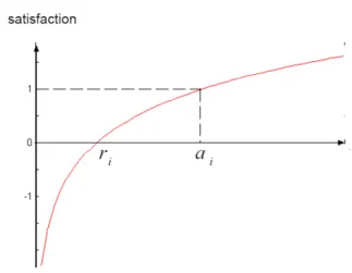
extension of the fuzzy membership function in terms of a strictly monotonic and concave utility function as shown in Figure 1 (see [11], [16], etc.)
We assume that the decision maker specifies requirements in aspiration and reservation levels by introducing desired and required values for several outcomes. Depending on the specified aspiration and reservation levels, aiand ri, respectively, we construct our achievement function ofθias follows:
µi(θi) = logαi θi ri , whereαi=ai ri . (15)
Formally, we defineµi(·) over the range [0, ∞), with µi(0) = −∞ andµ0
i(0) = ∞. Depending on the specified reference levels, this achievement function can be interpreted as a measure of the decision maker’s satisfaction with the value of the i-th
Figure 1: The Graph of an Achievement Functionµi(θi)
criteria. It is a strictly increasing function ofθi, having value 1 ifθi= ai, and value
0 ifθi= ri. The achievement function can map the different criterion values onto
a normalized scale of the decision maker’s satisfaction. Moreover, the logarithmic achievement function will be intimately associated with the concept of proportional fairness (see [5], [11], and [12].)
Proposition 1. The achievement functionµi(θi) is continuous, increasing, and con-cave.
These results are entirely consistent with those assumptions on the utility func-tions for end-to-end flow control in [5], where the objective is to maximize the ag-gregate source utility over their transmission rates. In addition, it takes an analytical approach devised to address decision-making problems where targets have been as-signed to all the attributes. In other words, the DM may seek a satisfactory and suffi-cient solution through it. A key element is the achievement function that represents a mathematical expression of the unwanted deviation variables. Moreover, when some conditions hold the corresponding solution represents a balanced allocation among the achievement of the different goals. We will formulate the mathematical model of the fair bandwidth allocation by using the achievement function in the following sections.
2.3 Multiple objectives of applying achievement functions
Achievement functions are derived on the basis of reference points to project an arbitrary point to the set of nondominated attainable solutions. The achievement function is constructed in such a way that if the reference point is dominated, the optimization will advance past the reference point to a nondominated solution. By using the concept of the utility functions as mentioned, we can construct the
achieve-ment functionsµT
class i. Given the weightβT
i andβiD of the throughput and delay for each class i andβT
i +βiD= 1 for eachβiT,βiD ∈ (0, 1). Then, for each class i, we consider the individual objective function fi:
fi(x) ,βT i µiT(θi) +βiDµiD( θi λi) =βT i logαT i θi rT i +βD i logαD i θi/λi rD i =βT i logθi rT i logαT i +βD i log θi λirDi logαD i = log(θi rT i ) β Ti
logαTi + log( θi
λirD i ) β Di logαDi = log[(θi rT i ) β Ti logαTi · ( θi λirD i ) β Di logαDi ] = log[ (θi) ( β Ti logαTi + β Di logαDi ) (rT i) ( β Ti logαTi )· (λirD i ) ( β Di logαDi ) ] = log[(θi)Gi Hi ]
=Gilogθi− log Hi
whereλirepresents the demand of bandwidth per unit time for class i. Let αT i , aTi/riT αD i , aDi /rDi and Gi,βiT/ logαiT+βiD/ logαiD be constant numbers as well as
Hi, (rTi) ( β Ti logαTi )· (λirD i) ( β Di logαDi ).
Noteθi, a function of x, is the bandwidths allocated to class i. The individual objec-tive function fiis the function of the allocation pattern x.
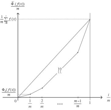
Next, it shows how to transform the multiple-objective problems to a single ob-jective optimization subject to the fairness for each class. We will apply an approach by analyzing aggregation of outcomes f(x) = ( f1(x), . . . , fm(x)). This approach is
in-troduced by Yager [21] as the so-called Ordered Weighted Averaging (OWA) Method. First, it defines the ordering map : Rm→ Rmsuch that
where
Φ1(f(x)) ≤ Φ2(f(x)) ≤ . . . ≤ Φm(f(x)).
There exists a permutationτ of set S ={1, 2, . . . , m} such that Φi(f(x)) = fτ(i)(x)
for i = 1, . . . , m. Then we define the cumulative ordering map ˜(f(x)) = ( ˜Φ1(f(x)),
. . ., ˜Φm(f(x))) defined as ˜Φi(f(x)) = ∑i
k=1Φk(f(x)), for i = 1, 2, . . . , m. The coeffi-cients of vector ˜(f(x)) express, respectively: the smallest outcome, the total of the two smallest outcomes, the total of the three smallest outcomes, etc. Vector ˜(f(x)) can be viewed graphically with a piecewise linear curve connecting point (0, 0) and points (i
m,
˜ Φi(f(x))
m ) for i = 1, 2, . . . , m. Such a curve represents the absolute Lorenz curve as shown in Figure 2. Fair solutions to problem (14) can be expressed as
m i 1 0 m 1 m 2
...
Figure 2: The Graph of a Absolute Lorenz Curve
Pareto-optimal solutions for the multiple criteria problem with objectives ˜(f(x)) max {( ˜Φ1(f(x)), ˜Φ2(f(x)), . . . , ˜Φm(f(x)) ) : x ∈ Q}. (16)
Theorem 2. A feasible solution x ∈ Q is a fair solution of the resource allocation problem (14), if and only if it is a Pareto-optimal solution of the multiple criteria problem (16).
2.4 Majorization
We introduce the concept of majorization (see [9], [10]) to provide the fairness. For the n-dimensional decision vector x=( x1, . . . , xn) of reals, let x(1) ≤ . . . ≤ x(n)
denote the components of x in increasing order. Definition 1. For x and y in Rn, x ≤My if ∑n
i=1x(i)= ∑ni=1y(i)and ∑ki=1x(i)≥ ∑ki=1y(i),
for k = 1, . . . , n − 1. When x ≤My then x is said to be majorized by y.
If x ≤My, then the allocation x is more fair than y. Next, we have the following definition.
Definition 2. A function g : Rn→ R is called Schur-concave, if x ≤
M y implies
g(x) ≥ g(y).
Thus, we present the following theorem which is adopted from [10].
Theorem 3. Let h be an arbitrary real function and define g(x)=∑n
i=1h(xi) for x ∈
Rn, then g is Schur-concave if and only if h is concave.
Recall that the achievement functions,µiand ˆµi, are concave functions. Accord-ing to this definition, it is easy to prove that the function fiis Schur-concave.
In the following, we will introduce the concept of fairness by using the fair aggregation function (see [5], [10], [11], [12], [21]). Typical solution concepts for
multiple criteria problems are defined by aggregation functions g : Rm→ R to be
maximized. Thus, (14) becomes
max{g(f(x)) : x ∈ Q} (17)
The simplest aggregation functions commonly used for the multiple criteria problem (14) are defined as the weighted sum of outcomes
g(f(x)) = m
∑
i=1wifi(x), (18)
or the worst outcome
g(f(x)) = min
i=1,...,mfi(x). (19)
An aggregation (17) is fair if it is defined by a strictly increasing and strictly Schur-concave function g.
Definition 3. An aggregation function g satisfying all the following requirements (20), (21) and (22), we call the corresponding problem (17) a fair aggregation of problem (14). For all i ∈ S = {1, 2, . . . , m},
g( f1(x), . . . , fi−1(x), fi0(x), fi+1(x), . . . , fm(x)) < g( f1(x), . . . , fm(x)), (20)
whenever f0
i(x) < fi(x). For any permutationπ of S,
g( fπ(1)(x), fπ(2)(x), . . . , fπ(m)(x)) = g( f1(x), f2(x), . . . , fm(x)) (21)
For any 0 <ε < zi0− zi00, we have
It is straightforward to see that g(f(x)) = ∑m
i=1wifiis a fair aggregation function according to this definition. Every optimal solution to the fair aggregation (17) of a resource allocation problem (14) defines some fair allocation scheme. In order to guarantee the consistency of the aggregated problem (17) with the maximization all individual objective functions in the original multiple criteria problem, the aggrega-tion funcaggrega-tion must be strictly increasing with respect to every coordinate, i.e., (20). In order to guarantee the fairness of the solution concept, the aggregation function must be additionally symmetric (impartial), i.e., (21). Symmetric functions satisfy-ing the requirement (22), are called strictly Schur-concave functions. Next, we give the following two theorems without proofs.
Theorem 4. For a strictly concave, increasing function µi: R → R, the function
g(f(x)) = ∑m
i=1wifi(x) is a strictly monotonic and strictly Schur-concave function.
Theorem 5. For a strictly concave, increasing function µi : R → R, the optimal
solution of the problem max{∑m
i=1wifi(x) : x ∈ Q} is a fair solution for resource allocation problem (14).
These proofs are omitted here due to the page limitation.
2.5 Mathematical models
In the following, we adopt an effective modeling technique for quantities ˜Φi(f(x)) with arbitrary i. In [11], for a given outcome vector f(x) the quantity ˜Φi(f(x)) may be found by solving the following linear program:
˜
Φi(f(x)) = max iti−
m
∑
k=1 dk subject to ti− fk(x) ≤ dk, k = 1, . . . , m dk≥ 0, k = 1, . . . , m, (23)where tiis an unrestricted variable and nonnegative variables dkrepresent their down-side deviations from the value of tifor several values fk(x). For example, the worst outcome of i = 1 may be defined by the following optimization:
˜
Φ1(f(x)) = max {t1: t1≤ fi(x) for i = 1, . . . , m }. (24)
Formula (23) provides us with a computational formulation for the worst con-ditional mean Mk
m(f(x)) defined as the mean outcome for the k worst-off services,
i.e., Mk m(f(x)) = 1 kΦk(f(x)), for k = 1, . . . , m.˜ (25) For k = 1, M1
m(f(x)) = ˜Φ1(f(x)) = Φ1(f(x)) which represents the minimum outcome.
For k = m, Mm m(f(x)) = 1 mΦm(f(x)) =˜ 1 m∑ m i=1Φi(f(x)) =m1∑ m
i=1fi(x) which represents the mean outcome.
For modeling various fair preferences one may use some combinations of the cumulative ordered outcomes ˜Φi(f(x)). In specific, for the weighted sum we obtain
m
∑
i=1wiΦi(f(x)).˜ (26)
Note that, due to the definition of map ˜Φi, the above function can be expressed in the
form with weightsνi= ∑m
j=iwi(i = 1, . . . , m) allocated to coordinates of the ordered
outcome vector. When substituting wiwithνi, (26) becomes ∑m
i=1νiΦi(f(x)), where ∑mi=1νi= 1 andνi≥ 0, ∀i = 1, . . . , m.
Applying the OWA method to problem (14), we get max {
m
∑
i=1νiΦi(f(x)) : x ∈ Q}. (27)
If weightsνiare strictly decreasing and positive, that isν1>ν2> . . . >νm−1>νm>
0, then each optimal solution of the OWA problem (27) is a fair solution of (14). Actually, formulas (23) and (26) allow us to formulate the following mathematical programming of the original multiple criteria problem:
maximize m
∑
i=1wiψi subject to ψi= iti−
m
∑
k=1 dki, ∀i = 1, . . . , m ti− dki≤ fk(x), ∀i, k = 1, . . . , m dki≥ 0, ∀i, k = 1, . . . , m tiunrestricted, ∀i = 1, . . . , m, x ∈ Q, (28)where wm=νm, wi=νi−νi+1for i = 1, . . . , m − 1,νi∈ (0, 1) for each i, and ∑mi=1νi=
1. The individual functionψi is the first i sum of the ordered multiple objective
functions (f(x)) in the allocation pattern x ∈ Q.
2.6 Piecewise linear form of the achievement functions
In implementation, it is convenient to handle a linear function rather than a concave function. Depending on the specified aspiration and reservation levels for each class i, ai and ri, respectively, we construct the achievement function ˆµi(θi)
of bandwidthθi as a piecewise linear function (29). Between ri and ai, We have
break points ri= ki,0≤ ki,1≤ . . . ≤ ki,n−1≤ ki,n= ai. We assume ki,l− ki,l−1are the same for all l = 1, . . . , n. Moreover, we denote the point bito represent the minimal bandwidth requirement for each class i. We will give the following propositions for the achievement function.
Lemma 6. Letκ be the cheapest cost per unit bandwidth given in an end-to-end
path. Suppose the total budget is B. There exists a finite number Mi≤ B/κKi such
Since pages are limited, proofs of the following results are skipped and will be
provided under request. We define ˆµi(·) over the range [0, Mi]. Depending on the
specified reference levels, this achievement function can be interpreted as a measure of the decision maker’s satisfaction with the value of the i-th criteria [7]. It is a strictly increasing function ofθi, having value 1 ifθi= ai, and value 0 ifθi= ri.
Practically, we define ˆµi(θi) = −M for 0 ≤θi< bi
ρ0· (θi− ki,0) for bi≤θi< ri
ρ1· (θi− ki,1) +µi(ki,1) for ri≤θi< ki,1 ρ2· (θi− ki,2) +µi(ki,2) for ki,1≤θi< ki,2 ..
.
ρn−1· (θi− ki,n−1) +µi(ki,n−1) for ki,n−2≤θi< ki,n−1 ρn· (θi− ki,n) + 1 for ki,n−1≤θi< ai
ρM· (θi− Mi) +µi(Mi) for ai≤θi≤ Mi.
(29)
Denoteαi=ai
ri, we have parametersµi(Mi) = logαiMi/riandµi(ki,l) = logαiki,l/rifor
l = 1, . . . , n−1. Moreover, the parametersρ0= M/(ri−bi),ρM= (µi(Mi)−1)/(Mi−
ai) and
ρl= n logαi(ki,l/ki,l−1)
ai− ri
, for l = 1, . . . , n,
represent the slope on l-th line segment for l = 0, 1, . . . , n and M. The slope of each segment represents a different marginal rate of satisfaction. The increasing (decreas-ing) rate case means that the DM wishes to attach a larger (smaller) marginal satis-faction depending on how far the achievement of the goal is from its target.
Next, we present an appealing property of the achievement function (15), which holds in the bandwidth allocation problem we are studying.
Proposition 7. The achievement function ˆµi(θi) is continuous, increasing, and con-cave.
Given the budget and a network, one may choose proper values of riand aisuch
thatθi∈ [ri, ai] for each connection, namely, the bandwidthθiin terms of transmission rates is always manageable between riand ai. Thus, ˆµi(θi) is well defined. Next, we focus on investigating the properties whenθi∈ [ri, ai].
Lemma 8. Let ˆµi(n)(θi) : [ri, ai] → [0, 1], where n means the number of break points,
be defined as the achievement function (15) restricted on [ri, ai]. Then the sequence
of functions { ˆµi(n)(θi)}∞
n=1converges uniformly toµi(θi) = logαi(θi/ri) on [ri, ai].
Proof. Letε > 0 be given. Choose N =(ri−ai)
ερM such that n ≥ N, implies
| ˆµi(n)(θ ) − µi(θi)| ≤| ˆµi(n)(ki,l) − ˆµi(n)(ki,l−1)| =|µi(ki,l) −µi(ki,l−1)|
=1 ρl|ki,l− ki,l−1| ≤ 1 ρM· ri− ai n <ε,
for eachθ ∈ [ri, ai]. The first inequality holds because both ˆµi(n)(θ ) and µi(θi) are increasing functions. Moreover, there must be an interval [ki,l−1, ki,l) ⊆ [ri, ai] contains θ for each θ ∈ [ri, ai]. Thus, by the definition of uniformly convergence, { ˆµi(n)}
converges uniformly to logαi(θi/ri) on [ri, ai]. ¤
Theorem 9. If ri≤θi≤ ai, then theε-proportionally fair bandwidth allocation ob-tained by using (15) as objective function approaches to proportional fairness as n → ∞.
Proof. When using the logarithm function logαi(θi/ri) as the associated objec-tive function for each class i, Luh and Wang [6] showed that this bandwidth allo-cation provided proportional fairness. By Lemma 8, the achievement function (15) converges uniformly to logαi(θi/ri). So, the fair bandwidth allocation, obtained by
using (15) as objective function, approaches to proportional fairness. ¤
The achievement function is intimately associated with the concept of propor-tional fairness. The achievement function (15) can also map the different criterion values onto a normalized scale of the decision maker’s satisfaction. When taking the achievement function which is considered as a measure of QoS on All-IP net-works, one can formulate the mathematical model of the fair bandwidth allocation in a network.
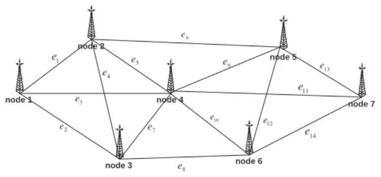
3 A Numerical Example
Consider a network topology G = (V, E) (as shown in Figure 3), where V = {node 1, node 2, . . ., node 7} and E = {ek, k = 1, 2, . . . , 14} denote the set of nodes and the set of links in the network respectively. Let node 1 and node 7 be the source and destination respectively. Each connection is delivered from o to d. Given the cost taking account of delay and the purchasing cost of bandwidth for each link: κ1= $5,κ2= $6,κ3= $10,κ4= $5,κ5= $4,κ6= $11,κ7= $6,κ8= $8,κ9= $6,
κ10 = $7, κ11 = $12, κ12= $6, κ13 = $5, and κ14= $6. There are also given the
maximal capacity of each link: U1= 2, 300 kbps (i.e. kilobits/sec), U2= 3, 500 kbps,
U3= 1, 000 kbps, U4= 2, 500 kbps, U5= 2, 100 kbps, U6= 2, 200 kbps, U7= 2, 000
kbps, U8 = 3, 000 kbps, U9 = 2, 100 kbps, U10 = 2, 700 kbps, U11 = 1, 500 kbps,
U12= 1, 800 kbps, U13= 3, 000 kbps, and U14= 3, 500 kbps.
There are given three classes (as Table 2 shows), where class 1 has the highest priority and class 3 has the lowest priority. The maximal possible number of connec-tions in each class is 10. Under the total available budget B = $130, 000, we want to allocate the bandwidths in order to provide each class with maximal possible quality of service (QoS) defined via (15).
node 2 node 7 node 6 node 3 node 5 node 4 node 1 1 e 2 e 3 e 5 e 6 e 9 e 4 e 8 e 14 e 13 e 11 e 12 e 10 e 7 e
Figure 3: Sample Network Topology
Table 2: The Characteristics of Each Class
class bandwidth requirement aspiration level of bandwidth reservation level of bandwidth reserved budget maximal number of connections 1 160 kbps 334 kbps 167 kbps $18,000 10 2 80 kbps 166 kbps 83 kbps $9,000 10 3 25 kbps 56 kbps 28 kbps $3,000 10
3.1 A Mathematical Programming
Let xkbe the bandwidth allocated to the link ek∀k = 1, 2, . . . , 14. We also letθi be the bandwidth allocated to the connection j of class i ∀i = 1, 2, 3. For each class i, we consider the objective function fias below:
f1(θ1) = log2 θ1 1670, (30) f2(θ2) = log2 θ2 830, (31) f3(θ3) = log2 θ3 280, (32)
whereθiis the bandwidth allocated to class i. Suppose each objective is regarded as
important as each other. Thus, each objective function has equal weight w1= w2=
w3=13. Then, we can formulate the mathematical model as follows.
As the formulation of (MP1), we have the following mathematical model (MP2):
maximize 1 3log2 θ1 1670+ 1 3log2 θ2 830+ 1 3log2 θ3 280 subject to 5x1+ 6x2+ 10x3+ 5x4+ 4x5+ 11x6+ 6x7+ 8x8+ 6x9 + 7x10+ 12x11+ 6x12+ 5x13+ 6x14= 130, 000 (10c1+ 18, 000) + (10c2+ 9, 000) + (10c3+ 3, 000) = 130, 000 θi· (5χi j(e1) + 6χij(e2) + 10χij(e3) + 5χij(e4) + 4χij(e5)
Figure 4: The Graph of f1(θ1)
Figure 5: The Graph of f2(θ2)
+ 11χi j(e6) + 6χij(e7) + 8χij(e8) + 6χij(e9) + 7χij(e10) + 12χi j(e11) + 6χij(e12) + 5χji(e13) + 6χij(e14)) = ci, ∀ j = 1, . . . , 10, ∀i = 1, 2, 3 θ1,1=θ1,2= · · · =θ1,10≥ 160 θ2,1=θ2,2= · · · =θ2,10≥ 80 θ3,1=θ3,2= · · · =θ3,10≥ 25 10
∑
j=1θi=θi, ∀i = 1, 2, 3
3
∑
i=1 10∑
j=1 χi j(ek) ·θi= xk, ∀k = 1, . . . , 14 χij(ek) = 0 or 1, ∀i = 1, 2, 3, ∀ j = 1, . . . , 10, and k = 1, . . . , 14 0 ≤ xk≤ Uk, ∀k = 1, . . . , 14,
where U1= 2, 300, U2= 3, 500, U3= 1, 000, U4= 2, 500, U5= 2, 100, U6= 2, 200,
U7= 2, 000, U8= 3, 000, U9= 2, 100, U10= 2, 700, U11= 1, 500, U12= 1, 800, U13=
3, 000, and U14= 3, 500.
3.2 Numerical experiments with ILOG
Since the objective functions fi in (30)-(32) are logarithmic functions which
can not be solved by ILOG software. To overcome this problem, we replace fi by
piece-wise linear functions ˆfifor each i = 1, 2, 3.
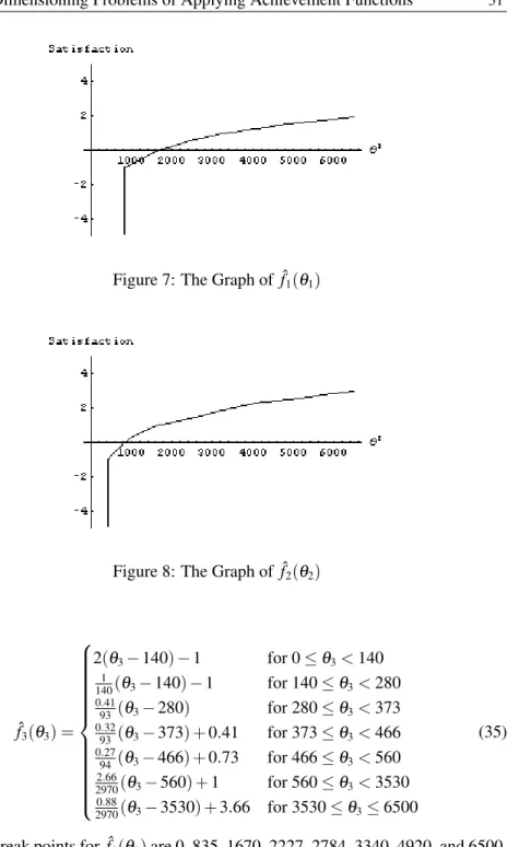
ˆf1(θi) = 2(θ1− 835) − 1 for 0 ≤θ1< 835 1 835(θ1− 835) − 1 for 835 ≤θ1< 1670 0.42 557(θ1− 1670) for 1670 ≤θ1< 2227 0.32 557(θ1− 2227) + 0.42 for 2227 ≤θ1< 2784 0.26 556(θ1− 2784) + 0.74 for 2784 ≤θi< 3340 0.56 1580(θ1− 3340) + 1 for 3340 ≤θ1< 4920 0.4 1580(θ1− 4920) + 1.56 for 4920 ≤θ1≤ 6500 (33) ˆf2(θ2) = 2(θ2− 415) − 1 for 0 ≤θ2< 415 1 415(θ2− 415) − 1 for 415 ≤θ2< 830 0.42 277(θ2− 830) for 830 ≤θ2< 1107 0.32 277(θ2− 1107) + 0.42 for 1107 ≤θ2< 1384 0.26 276(θ2− 1384) + 0.74 for 1384 ≤θ2< 1660 1.30 2420(θ2− 1660) + 1 for 1660 ≤θ2< 4080 0.67 2420(θ2− 4080) + 2.30 for 4080 ≤θ2≤ 6500 (34)
Figure 7: The Graph of ˆf1(θ1)
Figure 8: The Graph of ˆf2(θ2)
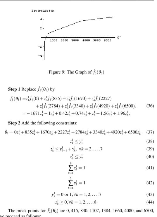
ˆf3(θ3) = 2(θ3− 140) − 1 for 0 ≤θ3< 140 1 140(θ3− 140) − 1 for 140 ≤θ3< 280 0.41 93 (θ3− 280) for 280 ≤θ3< 373 0.32 93 (θ3− 373) + 0.41 for 373 ≤θ3< 466 0.27 94 (θ3− 466) + 0.73 for 466 ≤θ3< 560 2.66 2970(θ3− 560) + 1 for 560 ≤θ3< 3530 0.88 2970(θ3− 3530) + 3.66 for 3530 ≤θ3≤ 6500 (35)
The break points for ˆf1(θ1) are 0, 835, 1670, 2227, 2784, 3340, 4920, and 6500,
Figure 9: The Graph of ˆf3(θ3) Step 1 Replace ˆf1(θ1) by ˆf1(θ1) =z11ˆf1(0) + z12ˆf1(835) + z13ˆf1(1670) + z14ˆf1(2227) + z1 5ˆf1(2784) + z16ˆf1(3340) + z17ˆf1(4920) + z18ˆf1(6500). = − 1671z1 1− 1z12+ 0.42z14+ 0.74z15+ z16+ 1.56z17+ 1.96z18. (36)
Step 2 Add the following constraints:
θ1= 0z11+ 835z12+ 1670z13+ 2227z41+ 2784z15+ 3340z16+ 4920z17+ 6500z18 (37) z1 1≤ y11 (38) z1 k≤ y1k−1+ y1k, ∀k = 2, . . . , 7 (39) z1 8≤ y17 (40) 8
∑
k=1 z1 k= 1 (41) 7∑
k=1 y1 k= 1 (42) y1 k= 0 or 1, ∀k = 1, 2, . . . , 7 (43) z1 k≥ 0, ∀k = 1, 2, . . . , 8. (44)The break points for ˆf2(θ2) are 0, 415, 830, 1107, 1384, 1660, 4080, and 6500,
we proceed as follows: Step 3 Replace ˆf2(θ2) by ˆf2(θ2) =z21ˆf2(0) + z22ˆf2(415) + z23ˆf2(830) + z24 ˆf2(1107) + z2 5ˆf2(1384) + z26ˆf2(1660) + z27ˆf2(4080) + z28ˆf2(6500). = − 831z2 1− 1z22+ 0.42z24+ 0.74z25+ z26+ 2.30z27+ 2.97z28. (45)
Step 4 Add the following constraints: θ2= 0z21+ 415z22+ 830z23+ 1107z42+ 1384z25+ 1660z26+ 4080z27+ 6500z28 (46) z2 1≤ y21 (47) z2 k≤ y2k−1+ y2k, ∀k = 2, . . . , 7 (48) z2 8≤ y27 (49) 8
∑
k=1 z2 k= 1 (50) 7∑
k=1 y2 k= 1 (51) y2 k= 0 or 1, ∀k = 1, 2, . . . , 7 (52) z2 k≥ 0, ∀k = 1, 2, . . . , 8. (53)The break points for ˆf3(θ3) are 0, 140, 280, 373, 466, 560, 3530, and 6500, we
proceed as follows: Step 5 Replace ˆf3(θ3) by ˆf3(θ3) =z31ˆf3(0) + z32ˆf3(140) + z33ˆf3(280) + z34 ˆf3(373) + z3 5ˆf3(466) + z36ˆf3(560) + z37 ˆf3(3530) + z38ˆf3(6500). = − 281z3 1− 1z32+ 0.41z34+ 0.73z35+ z36+ 3.66z37+ 4.54z38. (54)
Step 6 Add the following constraints:
θ3= 0z31+ 140z32+ 280z33+ 373z43+ 466z35+ 560z36+ 3530z37+ 6500z38 (55) z3 1≤ y31 (56) z3 k≤ y3k−1+ y3k, ∀k = 2, . . . , 7 (57) z3 8≤ y37 (58) 8
∑
k=1 z3 k= 1 (59) 7∑
k=1 y3 k= 1 (60) y3 k= 0 or 1, ∀k = 1, 2, . . . , 7 (61) z3 k≥ 0, ∀k = 1, 2, . . . , 8. (62)Next, combining (36), (45), and (54), we can replace the objective function 1 3log2 θ1 1670+ 1 3log2 θ2 830+ 1 3log2 θ3 280
by 1 3 ˆf1(θ1) + 1 3 ˆf2(θ2) + 1 3 ˆf3(θ3) = 1 3(−1671z 1 1− 1z12+ 0.42z14+ 0.74z15+ z16+ 1.56z17+ 1.96z18) +1 3(−831z 2 1− 1z22+ 0.42z24+ 0.74z25+ z26+ 2.30z27+ 2.97z28) +1 3(−281z 3 1− 1z32+ 0.41z34+ 0.73z35+ z36+ 3.66z37+ 4.54z38)
We proceed to consider the following constraints: θi· (5χi j(e1) + 6χij(e2) + 10χij(e3) + 5χij(e4) + 4χij(e5) + 11χi j(e6) + 6χij(e7) + 8χij(e8) + 6χij(e9) + 7χij(e10) + 12χi j(e11) + 6χij(e12) + 5χji(e13) + 6χij(e14)) = ci, ∀ j = 1, . . . , 10, ∀i = 1, 2, 3 (63) and 3
∑
i=1 10∑
j=1 χi j(ek) ·θi= xk, ∀k = 1, . . . , 14. (64) Since 0-1 variablesχij(ek) multiplied by decision variablesθi are nonlinear, we re-placeχi
j(ek)θiby nonnegative variables Aij(ek). Then (63) and (64) become 5Ai j(e1) + 6Aij(e2) + 10Aij(e3) + 5Aij(e4) + 4Aij(e5) + 11Ai j(e6) + 6Aij(e7) + 8Aij(e8) + 6Aij(e9) + 7Aij(e10) + 12Ai j(e11) + 6Aij(e12) + 5Aij(e13) + 6Aij(e14) = ci, ∀ j = 1, . . . , 10, ∀i = 1, 2, 3 (65) and 3
∑
i=1 10∑
j=1 Ai j(ek) = xk, ∀k = 1, . . . , 14. (66) Simultaneously, θ1,1=θ1,2= · · · =θ1,10≥ 160, (67) θ2,1=θ2,2= · · · =θ2,10≥ 80, (68) and θ3,1=θ3,2= · · · =θ3,10≥ 25 (69)can be rewritten respectively as A1
A2
j(ek) ≥ 80χ2j(ek), ∀k = 1, . . . , 14, ∀ j = 1, . . . , 10, (71) and
A3
j(ek) ≥ 25χ3j(ek), ∀k = 1, . . . , 14, ∀ j = 1, . . . , 10. (72) Then we have the constraints of the form
− A1 j(ek) + 160 ≤ 0 (73) − A1 j(ek) ≤ 0, (74) − A2 j(ek) + 80 ≤ 0 (75) − A2 j(ek) ≤ 0, (76) and − A3 j(ek) + 25 ≤ 0 (77) − A3 j(ek) ≤ 0. (78)
Adding the two constraints (79) and (80) to the model will ensure that at least one of (73) and (74) is satisfied:
− A1
j(ek) + 160 ≤ M ·χ1j(ek) (79)
− A1
j(ek) ≤ M · (1 −χ1j(ek)). (80)
Similarly, adding the two constraints (81) and (82) to the model will ensure that at least one of (75) and (76) is satisfied:
− A2
j(ek) + 80 ≤ M ·χ2j(ek) (81)
− A2
j(ek) ≤ M · (1 −χ2j(ek)). (82)
Next, adding the two constraints (83) and (84) to the model will ensure that at least one of (77) and (78) is satisfied:
− A3
j(ek) + 25 ≤ M ·χ3j(ek) (83)
− A3
j(ek) ≤ M · (1 −χ3j(ek)). (84)
In (79)-(84),χi
j(ek) is a 0-1 variable for each i, j and M is a number chosen large enough to ensure that
−A1 j(ek) + 160 ≤ M, −A1 j(ek) ≤ M, −A2 j(ek) + 80 ≤ M, −A2 j(ek) ≤ M, −A3 j(ek) + 25 ≤ M,
and
−A3
j(ek) ≤ M are satisfied.
From the above discussion, we present a Mixed-Integer programming model (MP3): maximize 1 3(−1671z 1 1− 1z12+ 0.42z14+ 0.74z15+ z16+ 1.56z17+ 1.96z18) +1 3(−831z 2 1− 1z22+ 0.42z24+ 0.74z25+ z26+ 2.30z27+ 2.97z28) +1 3(−281z 3 1− 1z32+ 0.41z34+ 0.73z35+ z36+ 3.66z37+ 4.54z38) subject to 5x1+ 6x2+ 10x3+ 5x4+ 4x5+ 11x6+ 6x7+ 8x8+ 6x9 + 7x10+ 12x11+ 6x12+ 5x13+ 6x14= 130, 000 (10c1+ 18, 000) + (10c2+ 9, 000) + (10c3+ 3, 000) = 130, 000 5Ai j(e1) + 6Aij(e2) + 10Aij(e3) + 5Aij(e4) + 4Aij(e5) + 11Ai j(e6) + 6Aij(e7) + 8Aij(e8) + 6Aij(e9) + 7Aij(e10) + 12Ai j(e11) + 6Aij(e12) + 5Aij(e13) + 6Aij(e14) = ci, ∀ j = 1, . . . , 10, ∀i = 1, 2, 3 − A1 j(ek) + 160 − Mχ1j(ek) ≤ 0, ∀ j = 1, . . . , 10, ∀k = 1, . . . , 14 − A1 j(ek) − M(1 −χ1j(ek)) ≤ 0, ∀ j = 1, . . . , 10, ∀k = 1, . . . , 14 − A2 j(ek) + 80 − Mχ2j(ek) ≤ 0, ∀ j = 1, . . . , 10, ∀k = 1, . . . , 14 − A2 j(ek) − M(1 −χ2j(ek)) ≤ 0, ∀ j = 1, . . . , 10, ∀k = 1, . . . , 14 − A3 j(ek) + 25 − Mχ3j(ek) ≤ 0, ∀ j = 1, . . . , 10, ∀k = 1, . . . , 14 − A3 j(ek) − M(1 −χ3j(ek)) ≤ 0, ∀ j = 1, . . . , 10, ∀k = 1, . . . , 14 10
∑
j=1θi=θi, ∀i = 1, 2, 3
3
∑
i=1 10∑
j=1 Ai j(ek) = xk, ∀k = 1, . . . , 14 χij(ek) = 0 or 1, ∀i = 1, 2, 3, j = 1, . . . , 10, and k = 1, . . . , 14 Ai
j(ek) ≥ 0, ∀i = 1, 2, 3, j = 1, . . . , 10, and k = 1, . . . , 14 0 ≤ xk≤ Uk, ∀k = 1, . . . , 14 θ1− 835z12− 1670z13− 2227z14− 2784z15− 3340z16− 4920z17− 6500z18= 0 θ2− 415z22− 830z23− 1107z24− 1384z25− 1660z26− 4080z27− 6500z28= 0 θ3− 140z32− 280z33− 373z34− 466z35− 560z36− 3530z37− 6500z38= 0 zi 1− yi1≤ 0, ∀i = 1, 2, 3
= 2100 = 2100 node 2 node 7 node 6 node 3 node 5 node 4 node 1 1 x 2 x 14 x 9 x 11 x 12 x = 0 = 0 = 0 = 0 = 0 = 0 = 0 = 0 = 2100 = 2100 = 2900 = 2900 = 2900 5 x 6 x 13 x 14 x 10 x 7 x 8 x 4 x
Figure 10: The Allocation of Bandwidths in Sample Network Topology
zi k− yik−1− yik≤ 0, ∀k = 2, . . . , 7, ∀i = 1, 2, 3 zi 8− yi7≤ 0, ∀i = 1, 2, 3 8
∑
k=1 zi k= 1, ∀i = 1, 2, 3 7∑
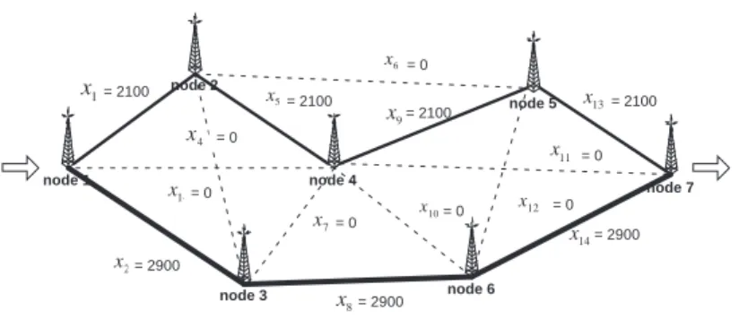
k=1 yi k= 1, ∀i = 1, 2, 3 yi k= 0 or 1, ∀k = 1, 2, . . . , 7, ∀i = 1, 2, 3 zi k≥ 0, ∀k = 1, 2, . . . , 8, ∀i = 1, 2, 3, where U1= 2, 300, U2= 3, 500, U3= 1, 000, U4= 2, 500, U5= 2, 100, U6= 2, 200, U7= 2, 000, U8= 3, 000, U9= 2, 100, U10= 2, 700, U11= 1, 500, U12= 1, 800, U13= 3, 000, and U14= 3, 500.Using this model, we can find a pareto optimal allocation of bandwidth on the network (as Figure 10) under a budget B = $130, 000. The Pareto optimal solution is: x3= x4= x6= x7= x10= x11= x12= 0 kbps, x1= x5= x9= x13= 2, 100 kbps,
x2= x8= x14= 2, 900 kbps, θ1, j= 300 kbps, θ2, j= 150 kbps,θ3, j= 50 kbps for
all j. We find the bandwidth allocated to class 1 isθ1= 3, 000 kbps, the bandwidth
allocated to class 2 isθ2 = 1, 500 kbps, and the bandwidth allocated to class 3 is
θ3= 500 kbps. This allocation can provide proportional fairness to every class, and
the satisfaction of each class equals 0.848. The optimal paths (in Figure 10) are 1-2-4-5-7 and 1-3-6-7, and the cost per unit bandwidth of the optimal path is $20. We also find the bottleneck links are e5and e9.
4 Conclusions
In this work, we present an approach for the fair resource allocation problem in All-IP networks that offer multiple services to users. Users’ utility functions are summarized by means of achievement functions. We find that the achievement func-tion can map different criteria onto a normalized scale. The achievement funcfunc-tion
also can work in the Ordered Weighted Averaging method. Moreover, it may be in-terpreted as a measure of QoS on All-IP networks. Using the bandwidth allocation model, we can find a Pareto optimal allocation of bandwidth on the network under a limited available budget, and this allocation can provide the so-called proportional fairness to every class. That is, this allocation can provide the similar satisfaction to each user in all classes. We also find the bandwidth allocated to each class.
Most of multiple criteria optimization reported in the literature use a weighted or a lexicographic achievement function. This selection is usually made in a mech-anistic way without theoretical justification. For each type of achievement function underlies a different philosophy on the DMs’ preferences. If the selection of the achievement function is improper, then it is very likely that the DM will not accept the solution. Therefore, the right choice of the achievement function is a key element for the success of the optimization model.
References
[1] A. M. S. Alkahtani, M. E. Woodward and K. Al-Begain. Prioritised best effort routing with four quality of service metrics applying the concept of the analytic hierarchy process. Computers & Operations Research, 33, 559–580, 2006. [2] Y. Bai and M. R. Ito. Class-based packet scheduling to improve QoS for IP
video. Telecommunication Systems, 29(1), 47–60, 2005.
[3] J. Gozdecki, A. Jajszczyk and R. Stankiewicz. Quality of service terminology in IP networks. IEEE Communications Magazine, 41(3), 153–159, 2003. [4] F. P. Kelly, A. K. Maulloo and D. K. H. Tan. Rate control for communication
networks: Shadow prices, proportional fairness and stability. Journal of the Op-erational Research Society, 49, 237–252, 1998.
[5] F. P. Kelly. Fairness and stability of end-to-end congestion control. European Journal of Control, 9, 159–176, 2003.
[6] H. Luh and C. H. Wang. Mathematical models of Pareto optimal path selection on All-IP networks. Proceedings of The First Sino-International Symposium on Probability, Statistics, and Quantitative Management, 185–197, 2004.
[7] H. Luh and C. H. Wang. Proportional bandwidth allocation for unicasting in All-IP networks. Proceedings of the 2nd Sino-International Symposium on Proba-bility, Statistics, and Quantitative Management, 111–130, 2005.
[8] M. Maher, K. Stewart and A. Rosa. Stochastic social optimum traffic assign-ment. Transportation Research Part B, 39, 753–767, 2005.
[9] A. W. Marshall and I. Olkin. Inequalties: Theory of Majorization and Its Appli-cations, Academic Press, New York, 1979.
[10] A. Müller and D. Stoyan. Comparison Methods for Stochastic Models and Risks, Wiley, Chichester, 2002.
[11] W. Ogryczak, T. ´Sliwi´nski, A. Wierzbicki. Fair resource allocation schemes and network dimensioning problems. Journal of Telecommunications and Informa-tion Technology, 3, 34–42, 2003.
[12] M. Pióro, G. Malicskó and G. Fodor. Optimal link capacity dimensioning in pro-portionally fair networks. NETWORKING 2002, LNCS 2345 277–288, 2002. [13] C. Romero. A general structure of achievement function for a goal programming
model. European Journal of Operational Research, 153, 675–686, 2004. [14] S. Sarkar and L. Tassiulas. Fair bandwidth allocation for multicasting in
net-works with discrete feasible set. IEEE Transactions on Computers, 53(7), 785– 797, 2004.
[15] R. E. Steuer. Multiple Criteria Optimization: Theory, Computation, and Appli-cation, Wiley, New York, 1986.
[16] A. C. Stockman. Introduction to Economics, 2nd ed., Dryden Press, Fort Worth, 1999.
[17] The UMTS Forun. Enabling UMTS/third generation services and applications. UMTS Forun Report, 11, 2000.
[18] C. H. Wang and H. Luh. Fair budget allocation of precomputation in All-IP networks. IFORS International Triennial Conference, Honolulu, Hawail, July 2005.
[19] W. Willinger and V. Paxson. Where Mathematics meets the Internet. Notices of the American Mathematical Society, 45(8), 961–970, 1998.
[20] X. Xiao and L. M. Ni. Internet QoS: A big picture. IEEE Network, March/April, 1999.
[21] R. R. Yager. On ordered weighted averaging aggregation operators in multicri-teria decision making. IEEE Transactions on Systems, Man and Cybernetics, 18(1), 183–190, 1988.
[22] R. R. Yager. On the analytic representation of the leximin ordering and its ap-plication to flexible constraint propagation. European Journal of Operational Research, 102, 176–192, 1997.