高度光線變化影響之影像的分析及處理技術開發

國 立 交 通 大 學

電機與控制工程學系

博

士

論

文

高度光線變化影響之影像的分析及處理技術開發

The Development of Analysis and Processing

Techniques for Images with Varying Lighting Effects

研 究 生：秦 群 立

指導教授：林 進 燈

高度光線變化影響之影像的分析及處理技術開發

The Development of Analysis and Processing

Techniques for Images with Varying Lighting Effects

研 究 生：秦群立 Student：Chiun-Li Chin

指導教授：林進燈 博士

Advisor：Dr. Chin-Teng Lin

國 立 交 通 大 學

電 機 與 控 制 工 程 學 系

博 士 論 文

A Dissertation

Submitted to Department of Electrical and Control Engineering

College of Electrical Engineering and Computer Science

National Chiao Tung University

in partial Fulfillment of the Requirements

for the Degree of

Doctor of Philosophy

in

Electrical and Control Engineering

January 2006

Hsinchu, Taiwan, Republic of China

高度光線變化影響之影像的分析及處理技術開發

摘要

隨著數位取像裝置(digital capture device)的技術日漸進步與使用者的日益增 加，功能的完善和價格便宜成為購買的重要條件。一般在攝影時使用者最關注的 三個方面分別是光線、焦距和色彩，所以對於自動曝光補償、自動對焦和自動白 平衡得功能要求也相對的提高，故本論文針對光線所引起的影像問題發展出新的 解決技術，首先，我們提出了一種文件影像二值化的方法，此方法會依據光線分 佈的強弱來決定適當的門檻值，我們利用同質性(Homogeneity)的方法將影像分 為兩個區域，再利用影像處理技術中的中值濾波器(Median filter)來得到最後的光 線分佈的強弱影像，依據此影像的指示配合我們所提出來的適應性門檻值決定的 演算法來做二值化，其所得到的結果與其他的方法比較可以發現我們所提出之方 法能夠避免光線的影響而得到一個完整的二值化影像。接下來我們提出了一個逆 光影像偵測與補償的演算法，逆光補償(Backlight compensation)是許多數位取像 裝置中都會提供的一個功能，但是其補償的效果不理想並且未有偵測的功能存 在，有鑑於此我們從影像的空間位置(Spatial position)和亮度分佈機率統計圖 (Histogram)抽取出兩個指示影像逆光程度的指標，利用模糊推論(Fuzzy inference) 的方法整合這兩個指標來完成逆光偵測。在逆光補償方面，我們提出利用曲線來 調整影像的亮度，此曲線可以提升逆光影像中主體的亮度，並讓影像中的其它部 份的亮度維持住，如此便能完成補償的動作，在此我們使用兩個數學方程式來描 述這個曲線，一個是拋物線方程式(Parabolic equation)，另一個是三次方程式 (Cubic equation)，從實驗的結果顯示使用三次方程式為補償曲線的結果比使用拋 物線方程式的結果好，因為它有更平滑的特性。

The Development of Analysis and Processing Techniques

for Images with Varying Lighting Effects

Student: Chiun-Li Chin Advisor: Chin-Teng Lin Department of Electrical and Control Engineering

National Chiao-Tung University

Abstract

This dissertation is aimed at the image problems with varying lighting effects. First, we have a new method of document Image binarization, and with this method we can decide the proper threshold value by the distribution of light, and we use this method of the homogeneity to separate the images into two parts, and then use one of the technology approaches, the Median filter, to get the very last image of light distribution. According to its directives, we match up with the algorithm decided by our proper threshold value to get a threshold, and try to compare the result with the one of the other methods, we found that our method can avoid the influence of light and has got a complete binarized image.

Subsequently, we proposed an algorithm of backlight image detection and compensation. Backlight compensation is the function which many digital capture devices would provide, but the effects of the compensation are not good enough to what we have expected, and even there was not the function of detection. Seeing that we choose two indicators of directing image backlight levels from the image spatial position and its histogram, by using the fuzzy inference, we integrate the two indicators to complete the backlight detection. In the backlight compensation, we suggest that using it to adjust the brightness of images because the curve can elevate the brightness of the main object, and keep the brightness of other parts. By that, we can complete the compensation. Herein, we use two formulas to describe this curve. One is the parabolic equation; the other is the cubic equation. From the results of the experiment, using the cubic equation to be the calculation of the compensation curve is better than using the parabolic one, because it has more flexible characteristic.

誌謝

Contents

Abstract ...ii

Contents ...iv

List of Figures ...vi

List of Tables... viii

1. Introduction...1

1.1. Motivation...1

1.2. Brief Introduction of the Relation between Light and Digital Camera ...1

1.3. Human Vision System...3

1.4. Concluding Remarks...6

2. An Adaptive Image Binarization Method for Camera-Based Document Images....7

2.1. Introduction...7

2.2. Obtaining Background Surface Image... 11

2.3. Adaptive Thresholding...14

2.3.1. Differencing ...15

2.3.2. Determining Threshold Value...16

2.4. Experimental Results and Discussions ...18

2.5. Concluding Remarks...23

3. Solving Backlight Image Problem with Fuzzy Logic and Compensation Curve ..24

3.1. Introduction...24

3.2. Backlight Detection Phase ...29

3.2.1. Backlight Index Based on the Spatial Characteristic of an Image...30

3.2.2. Backlight Index Based on the Histogram Characteristic of an Image ...32

3.2.3. Fuzzy Integration of Two Backlight Indices...34

3.4. Backlight Image Compensation with a Compensation Curve ...36

3.4.1. The Inspiration ...36

3.4.2. Compensation Curve Consists of Two Parabolas...36

3.4.3. Compensation Curve Based on Cubic Equation...38

3.4.4. Turning Point or Inflection Point Searching...41

3.5. Experimental Results and Discussions ...43

3.6. Concluding Remarks...51

4. Conclusions and Perspectives ...52

References...53

List of Figures

Figure 1.1 The image histogram. ...2 Figure 2.1 The system flowchart of our proposed method. ...10 Figure 2.2 The course of image binarization with different threshold value. ... 11 Figure 2.3 The first row is original images and the second row is processed images by homogeneity pixel detection and recursive median filter. ...14 Figure 2.4 A scheme of adaptive thresholding...15 Figure 2.5 The first row shows original image and its histogram and the second row shows processed image by median filter and its histogram. ...16 Figure 2.6 (a) and (b) are original and background surface image, respectively. (c) is difference image. (d) is histogram of difference image. (e) is final result image with adaptive thresholding method. ...18 Figure 2.7 The samples of testing images in our image database for the experiments of our proposed image binarization algorithm. ...21 Figure 2.8 (a) and (c) are original images. (b) and (d) are processed images by global thresholding technique with Otsu’s threshold selection algorithm. ...21 Figure 2.9 The first row shows original image and the second row shows the

processed image by our proposed method. ...22 Figure 3.1 System architecture for detecting and compensating backlight images. ....28 Figure 3.2 Two representative backlight images and their histograms...29 Figure 3.3 The division of a backlight image. ...32 Figure 3.4 The representative histogram of backlight images. ...34 Figure 3.5 The membership functions of the fuzzy terms of B

hist, Bimage and BF.

...35 Figure 3.6 Adaptive curve for image compensation. ...38 Figure 3.7 (a) Cubic curve with the condition of a>0. (b) Cubic curve with the

condition of a<0. (c) Cubic curve with violent curvature. (d) Cubic curve with normal curvature. (e) Cubic curve with over-smooth curvature...39 Figure 3.8 Histograms of two representative backlight images...43 Figure 3.9 (a) to (d) are original images, (e) to (h) are the compensated images by our method, and (i) to (l) are the compensated images by the method in [27]. ...47 Figure 3.10 (a) to (d) are four original backlight images, (e) to (h) show the

compensated images by our proposed method, and (i) to (l) show the compensated images by the histogram equalization method...48 Figure 3.11The column (a) shows the original images, Column (b) shows the

segmented images, Column (c) shows the compensated images by the segmentation method, and Column (d) shows the compensated images by our proposed method...49 Figure 3.12 (a) to (d) are original images, (e) to (h) are the compensated images

obtained by our old method in Ref. [23], and (i) to (l) are the compensated images by our new method. ...50

List of Tables

Table 1 Comparison between our proposed method and others method with Precision and Recall...22 Table 2 Representative processed results after applying several binarization schemes with Levenshtein distance...22

1. Introduction

1.1. Motivation

With the technology of digital capturing device progressing at an extremely rapid pace, the solving of digital camera and digital video device problems increases in importance. These problems include Auto-Focus (AF), Auto-Exposure (AE) and Auto-White Balance (AWB) as well as others. Light is one of the main actors causing these problems; it is the basis of all photography. Without light, we are all left in the dark. Adaptations to darkness and light are the basic visual sensitivity changes related to the increase or the decrease of the level of illumination. Image capturing systems do not have the ability to adapt to an illumination source. Therefore, illumination sources captured by digital cameras may vary according to the scene, and often within the scene. Consequently the motive of this thesis is to solve the previously mentioned problem caused by light in the image.

1.2. Brief Introduction of the Relation between Light and

Digital Camera

All digital cameras have an automatic mode that sets the focus, the exposure and the white-balance for the user. All the latter needs to do is to frame the image and push the shutter-release button. This auto mode of operation is great in the majority of the situations; it lets us focus on the subject instead of the camera.

the light or darkness will affect the photograph. When the shutter opens, light (reflected from the subject and focused by the lens) strikes the image sensor inside the camera. If too much light strikes it, the photograph will be overexposed, washed out and faded looking. On the contrary, too little light produces an underexposed photograph, dark and lacking in details, especially in shadow areas. If there is light behind a subject and a photographer standing in front of the latter takes a picture, a backlight image will be produced.

The amount of light that exposes the image can be controlled with the adjustment of either the aperture (the size of the opening through which light enters the camera) or the shutter speed (the length of time light is allowed to enter). With the automatic exposure control function, the camera can make one or both of these adjustments for the user. All digital cameras give us fully automatic operations so we only need point and shoot to take pictures. These automatic systems are great in the vast majority of situations and even the best photographers use them frequently. For more creative control, however, we need to be able to override the auto settings.

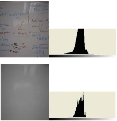
Many cameras now display histograms, which let the user evaluate the distribution of tones. Figure 1.1 shows an image histogram. Since most of the image corrections can be diagnosed by looking at a histogram, it helps to look at it while one is still in a position to re-shoot the image. Each pixel in an image can be set to any of the 256 levels of brightness from pure black (0) to pure white (255). It is a graph that shows how the 256 possible levels of brightness are distributed in the image.

The horizontal axis represents the range of brightness from 0 on the left to 255 on the right. Think of it as a line with 256 spaces on which to stack pixels of the same brightness. Since these are the only values that can be captured by the camera, the horizontal line also represents the camera's maximum potential dynamic range.

The vertical axis corresponds to the amount of pixels that each one of the 256 brightness values has. The higher the line coming up from the horizontal axis is, the more pixels there are at that level of brightness.

To read the histogram, the user needs to look at the distribution of pixels. An image that uses the entire dynamic range of the camera will have a reasonable amount of pixels at every level of brightness. An image that has a low contrast will have the pixels clumped together and a narrower dynamic range. Whilst a backlight image will have two pixels clumped. The first distributes the low brightness area and the other distributes on high brightness area.

1.3. Human Vision System

Eyes play an important role in our life, not only for seeing objects present in our surrounding world, but also for reading letters, looking at paintings, photographs, films, etc. The eye’s visual acuity is generally believed to be the most important factor regarding the ability of the eye to see objects. Acuity is usually measured with tests (acuity tests) i.e. recognition of different sized black letter at a certain distance, measurement of the minimum visible separation of black rings with a small interrupted part. These tests are used to prescribe certain type of eyeglasses, however they give no information about the series of other factors that also play a role in the human visual system.

emitting psychic matters, and that vision was a process of feeling the scene. This led the early anatomists to regard the optic nerve as a hollow tube through which the substance was transmitted. In the past, scientists always compared the eye to a camera, a darkened chamber with the image focused on its rear surface; inverted image of the scene were then observed on this area. In fact this observation created its own problems. Since we do not invert images, the active region for seeing was assumed to be the lens rather than the retina. This confusion arose from the ignorance that humans do not see the retinal image but rather see with the aid of it. The eye is not simply an instrument used to record images; it acts as optical interface between the environment and the neural elements of the visual system. It provides the basic attributes for vision i.e. forms, fields, colors, motions, and depths.

Visual perception results from a series of optical and neural transformations. The cornea and the lens first transform light reaching the eye, focusing light and creating a retinal image. The retinal image is then transformed into neural responses by the photoreceptor, light-sensitive elements of the eye. The photoreceptor responses are transformed into several neural representations within the optic nerve, the latter transformed into a multiplicity of cortical representations.

The human visual system is a remarkable apparatus, which allows us to perceive objects under a wide range of ambient illumination, from starlight to daylight, with a resolving power of up to 1'. However, it has several important limitations, which we need to be aware of in the context of displaying high-dynamic range content. It is useful over a wide range of luminance values; at any given time one can perceive no more than 5 orders of magnitude of dynamic range. With the effect of time-adaptation, this range can be shifted up and down to cover 10 orders of magnitude. Despite the wide visual field of view of the human eye, it is not possible to observe the whole scene simultaneously. Rather, we sequentially focus our attention on local areas of the

field of vision, where the eye rapidly adapts itself to the average brightness in the neighborhood of 1–1.5° of visual angle centered at the fixation point. The luminance adaptation determines which part of the overall intensity range will be most sensitive for the eyes at a given moment.

Furthermore, there is a limit to how much contrast can be perceived in a very small neighborhood of the visual field. That is, when the contrast between adjacent spots on the retina exceeds a particular threshold, the eyes will no longer be able to perceive the relative magnitude of that contrast (roughly speaking, the spot on one side will appear white and the one on the other – black). If one separates the spots in space, the latter will be able to see the variations in brightness. The threshold at which this occurs, the maximum perceived contrast, is reported to be around 150:1.

Another major cause of human inability to distinguish detail in areas of high contrast is called disability glare. It is caused by light scattering inside the liquid medium of the eye, in the atmosphere, and sometimes the surface of the display. The effect of disability glare forms a constant veiling luminance across a large part of the image area that obscures any detail that has a lower luminance value.

1.4. Concluding Remarks

In this chapter, we introduced basic concepts such as light, digital camera and human vision system. The main purpose the latter concept explanation is that they are related to the proposed methods of this thesis. We will deal with two categories, the image-document and the natural image including landscape and portrait. Herein, the capturing device is the very popular digital camera. Firstly, the linearization in document image processing is of great importance. It is a pre-processing step that affects the result of segmentation. Therefore, we propose an effective binarization method, which will be described in the chapter 2. In the chapter 3, we propose a backlight image detection and compensation method. In the compensation part, two methods are proposed. (For details see section 3.4.2 and 3.4.3 of Chapter 3) All digital cameras have the backlight image compensation function, however they do not have the detecting function. The compensation effect does not satisfy every user. Our proposed method can be effective to solve these problems. Finally, conclusions and perspectives are described in the last chapter.

2. An Adaptive Image Binarization Method for

Camera-Based Document Images

In this Chapter, we propose a new algorithm for camera-based document image binarization based on an innovative analytic model. The development of this algorithm results from the observation of the ring phenomenon caused by light variation in the document images. Due to the existence of such phenomenon, the image threshold becomes difficult. As a result, three methods can be used to achieve image binarization i.e. image homogeneity pixel search, recursive median filter method and adaptive threshold selection. Firstly, the search of image homogeneity pixel serves to classify image pixel into two classes. Its objective is to speed up the action of recursive median filter. The recursive median filter resolves the traditional median filter problem that stop criterion and use it to obtain a background surface image. Subsequently, using adaptive threshold selection method helps select different threshold value according to the background surface direction. Finally, we will get foreground image. Extensive experimental results have shown that the proposed algorithm can binarize the background of various kinds of document images without discarding practicable information.

2.1. Introduction

This research main motivation comes from the convenience of using digital cameras as opposed to conventional scanning devices. Cameras occupy little space on a user’s desk, provide excellent feedback for alignment, capture immediately the

image and allow documents to be scanned face up. Moreover, since cameras acquire images under less constrained conditions than devices specifically designed for high-quality document capture, they can introduce severe image variations and degradations, making it especially hard to obtain reliable OCR result from these images. Hence the aim of this paper is to design an adaptive binarization algorithm specifically for OCR of camera image.

Many methods for the binarization of document image exist, such as wavelet transforms, thresholding techniques, and the statistical analysis methods, etc. Wavelet transforms use the decomposition analysis of different levels to remove noise. Its key point lies on the choice of basis functions. From the papers [1][2][3], we found it required higher time complexity by using wavelet transforms with common basis functions such as Haar function and Daubetch spline function.

Two modes are usually used for thresholding. The first one, the global thresholding, finds a single threshold for all image pixels. These methods are general but not robust. Actually, it is very fast and efficient when the pixel values of the components and those of the background are fairly consistent. The second one, the local thresholding, uses different threshold values that are required for different local areas. These methods are more robust but not as general due to the large amounts of parameters needed to be tuned. Although many thresholding techniques [4] [5] [6] [7] [15], such as global [10] and local ones [8][9], have been developed in the past, it is still difficult to deal with low quality images. Meanwhile, in this context, or in general, documents processing systems need to process a large number of documents with different style, thus, they require that the whole processing procedure is achieved automatically and without prior knowledge and pre-specified parameters. Using an approach similar to the one used in this thesis, Sauvola [12] processed only uneven lighting in time-domain. Yang [16] developed a thresholding method based on

gradient with edge preservation on poor quality documents without complex backgrounds. Seeger [13] created a new thresholding technique for camera images, like in this context, by computing a surface of background intensities and by performing adaptive thresholding for simple backgrounds. This discordance between the threshold and the characteristics of the image usually leads to an unsatisfactory result.

In [14], the proposed technique by histogram modification includes two common methods, the first is the histogram equalization, the second is the histogram normalization. These methods differ one from another on the choices of the output functions. The decision of output functions will change the distribution of probability, and later change the properties of the original images, although they could increase the intensity of an image and solve the problems of various intensity uniformity of an image. All of these simplify the understanding that the histogram modification can indicate some tiny information from the document image.

For a long time, we have been able to get various document images by scanning. But incessant advance in the digital techniques have made digital cameras the most popular tool to capture document images. Due to the lens and the environmental light that can affect document image obtained by the digital camera, the previously proposed methods are not suitable directly to binarize a document image obtained by digital cameras. Therefore, this paper presents a simple but novel adaptive document image binarization algorithm that achieves considerably better OCR performance than the other methods, while being more runtime efficient. The proposed scheme consists of three main steps. The first step is to classify image pixel into two classes, homogeneity or non-homogeneity. This objective is to speed up algorithm speed. Subsequently, it is to obtain background surface image by recursive median filter according to the first step result. Final step is the adaptive thresholding. The whole

system flow is showed in the Figure 2.1.

This chapter is organized as follows. Section 2.2 describes how to obtain a background surface in a document image. Section 2.3 proposes an adaptive thresholding selection method, which is employed to determine optimal threshold value based on background surface of image. Section 2.4 provides and discusses the experimental results. Finally, Section 2.5 gives conclusions and suggestions for some future works.

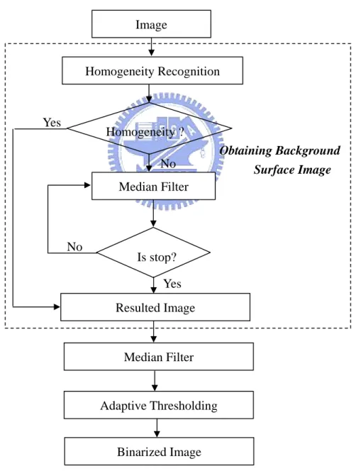
Figure 2.1 The system flowchart of our proposed method.

Obtaining Background Surface Image Image Adaptive Thresholding Binarized Image Median Filter Is stop? Yes No Homogeneity Recognition Homogeneity ? Yes Resulted Image No Median Filter

2.2. Obtaining Background Surface Image

An important problem for thresholding methods comes from a non-uniform

illumination which introduces most of the noise when using only a global method.

Figure 2.2 shows a processed result of document image captured by digital camera. People believe that the document image can be simply processed with simple image thresholding method. However, it is just the opposite. We discovered that the image is affected by the environment’s variation of illumination. The latter is able to find the light variation out with different threshold value. Hence, this problem cannot be simply solved with the use of the traditional global or local thresholding methods.

There are many image processing methods that can be applied to solve image binarization problems, i.e. local thresholding or clustering. But, the processed results are usually not good enough. Therefore, the present research proposes a method to obtain background surface of image in order to overcome environment illumination effects. This proposed method is divided into two parts. The first one is the employment of the detection method of image homogeneity pixel, to classify image pixel into two classes, homogeneity or non-homogeneity. Then, using recursive median filter, obtain a background surface image of document image. Finally, we propose an adaptive thresholding method to get a binarized image whose background is removed.

Figure 2.2 The course of image binarization with different threshold value. For the first step, we want to obtain a background surface image. This surface

can show the variation of illumination in the image. In general, it needs many methods to achieve this task, i.e. edge detection, interpolation. This is a kind of complicated procedure. For reducing complexity, we will divide it into two parts. First, we detect the property of homogeneity of each pixel in the image. Second, the median filter is used to do smoothing task. It is analogous to interpolation action. The median filter is normally used to reduce noise in an image, somewhat like the mean filter. However, it often does a better job than the mean filter of preserving useful detail in the image.

There are two important problems noticed when using median filter: mask size and iteration number. The iteration number indicated how many times we perform median filter to whole image. First, the small mask size should be selected because we have to obtain the detailed part in the image. Hence, for this work, we select the mask size empirically. In our experiment, unless stated otherwise, the mask size for the median filter is set from 7*7 or 9*9 and the recursive number is decided by the following formula:

(2.1)

ε

<

×

−

∑∑

n

m

I

I

The m and n represent the image height and width, respectively. The ε is a threshold value. Herein, we set this value to 0.01. The I_mnt represents an image that has resolution of m×n at time t. When the difference between the current image processed by median filter and previous image processed by median filter is less than the one from the threshold value, the median filter’s operation stops. The whole procedure for obtaining the background surface image goes as followed:

(2.2)

1

σ

σ

e

e

H

=

−

×

(2.3)

,

)

(

n

1

I

m

e

G

G

+

=

−

=

∑

σ

where H can depict a pixel as homogeneity or non-homogeneity [19]. _i

From equation 2.2, we can see that the H value ranges from 0 to 1. _i

The higher the H value is, the more homogenous the region _i

surrounding the pixel i is. In the equation 2.2, the σ_i represents a standard deviation at pixel i and the σ_max is maximum value in the all

i

σ . In the equation 2.3, the m is the mean of _i n intensities within the window w and the _d e represents a measure of discontinuity around _i

pixel i . The e_max is maximum value in the all e . In the _i e , the _i G _x

and G are gradients at pixel i in the x and y direction. _y

Step 2: We have to set a threshold value toH . If _i H is larger than 0.95, then _i

the pixel i is a homogeneity point. Herein, the value 0.95 is determined

by our experiment. The pixel it has to do median filter.

Step 3: The pixel which has to do median filter need to be determined whether it should stop to do median filter with equation 2.2. If stop to do median filter go to step, then go to step 1.

Step 4: Finally, median filter is applied to whole image against.

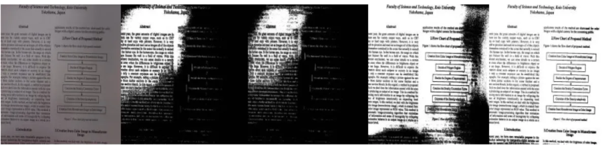
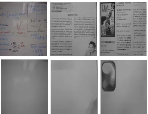
The first row of Figure 2.3 shows the original image and its second row shows the processed result by homogeneity pixel detection and recursive median filter.

Figure 2.3 The first row is original images and the second row is processed images by homogeneity pixel detection and recursive median filter.

2.3. Adaptive Thresholding

At this step, we proceed to get the final threshold value by combining the calculated background surface B with the original image I. Figure 2.4 shows the our

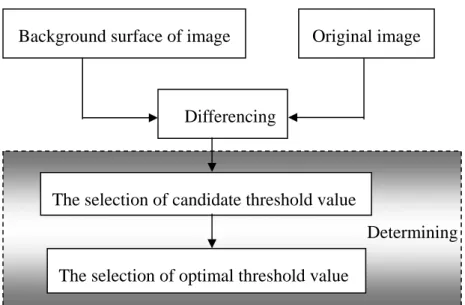
proposed whole flowchart of adaptive thresholding. The determination of threshold value is divided into two steps: differencing and determining threshold value. The determining threshold value consists of the selection of candidate threshold value and the selection of optimal threshold value.

Figure 2.4 A scheme of adaptive thresholding.

2.3.1. Differencing

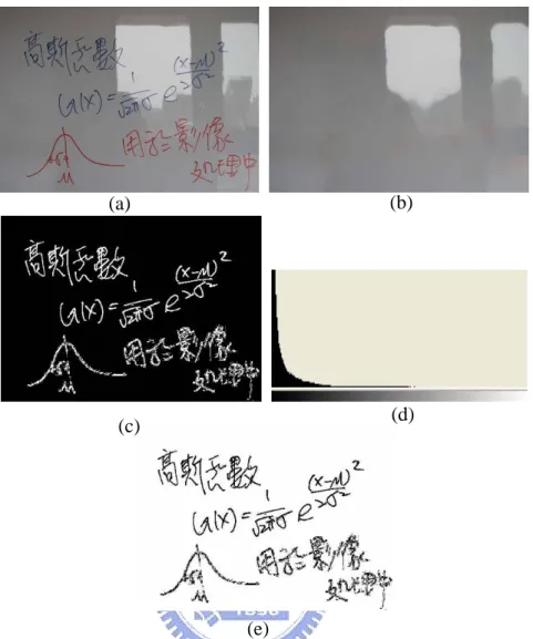
After getting the background surface image, by comparison, we discovered that the image is really a background part of the original image from comparing histogram between this image and original image. Figure 2.5 shows this result. Hence, we want to subtract background surface part from original image. It makes it easy for getting threshold value of image. In general, there are two subtraction methods used. The first is to directly do the subtraction between two images. The other is calculating difference between two images. We adopt the differencing method here. The first, the two images are to do subtraction operation. Next, the result is taken in absolute value. We discovered that the image histogram becomes very simple when we perform differencing operation to the two images. This is conducive to search threshold value. Figure 2.6 (c) shows the result image of differencing between Figure 2.6 (a) and (b). Figure 2.6 (d) shows the histogram of differencing image.

Background surface of image Original image

Differencing

The selection of candidate threshold value

The selection of optimal threshold value

Figure 2.5 The first row shows original image and its histogram and the second row shows processed image by median filter and its histogram.

2.3.2. Determining Threshold Value

In this section, we need to find the all candidate threshold values. The reason is to speed up the selection speed of optimal threshold value. Generally, the algorithm of threshold value selection will search all gray value in the image, and then the optimal threshold value will be found after the first one by bye the one calculating. Hence, the determination of optimal threshold value needs to take more time. For solving this problem, we use the selection method of candidate threshold value to obtain candidate threshold value before determining the optimal threshold value. It can speed it up for optimal threshold value determination. The algorithm can be divided into several steps as the follows.

between every term in the Hist matrix which is obtained by calculating

the histogram of differencing image. The sign(•) represents sign function.

Setp2: Generally, optimal threshold value occurs in the valley of histogram. Hence, we search all valleys probable becoming optimal threshold in the histogram. It should be as follow:

valley ={i+1|H(i) = −1and H(i+1) =1,i =0~ 255}

Setp3: People feel darkness at a value of intensity less than 60 according to human vision characteristic [22]. Hence, we only remain the valley value of gray level value less than 60. These values are candidate threshold values and they will be substituted in next step.

Subsequently, when having found the all candidate threshold values, we will pick up an optimal threshold value from the all candidates. The Otsu’s method [10] is based on a discriminant analysis, which maximizes the ratio of the between class variance to the total variance to obtain thresholds. In thresholding of gray-level image, it is efficient on the basis of uniformity measure between the two classes that should be segmented. So it provides an appropriate mean to analyze further aspects other than the selection of the optimal threshold for a given image. However, this method needs to search all the histograms of image for getting optimal threshold value. This takes a long time and it is very complex to finish optimal threshold value searching. Hence, we use the selection method of candidate threshold value to get an optimal threshold value. The proposed method is to speed up searching time. The optimal threshold value is selected from these candidates. We will not need to search the whole the histogram of differencing image.

Figure 2.6 (a) and (b) are original and background surface image, respectively. (c) is difference image. (d) is histogram of difference image. (e) is final result image with adaptive thresholding method.

2.4. Experimental Results and Discussions

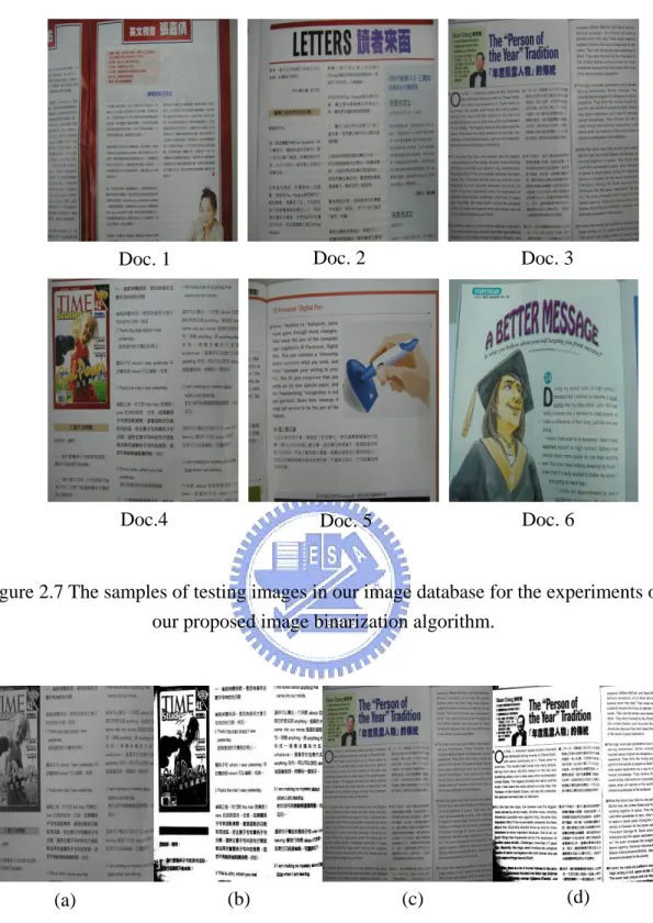
In the above, we proposed an approach for binarizing camera-based document image. We used 200 images with the size 1536*2176 for testing our algorithm. These images include the ones with the background in light colors and slightly white colors, taken by the Fujifilm FinePix 6800 Zoom digital camera. Figure 2.7 represents some part of our testing images. Our proposed algorithm is performed under Pentium 4 1.2G HZ CPU. It will take at most 0.5 second to finish the whole algorithm for each image. Therefore, our algorithm can rapidly process high-resolution images.

(a) (b)

(c) (d)

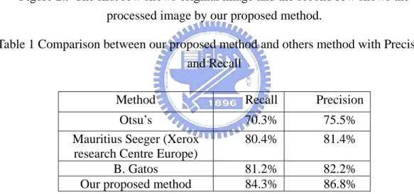
Figure 2.8 (a) and (c) are the original document image, and Figure 2.8 (b) and (d) are the processed image after using the general global thresholding method. Herein, the Otsu’s threshold selection method is used as global thresholding method. Although most of the background information is removed, we still observe two major problems. First, the information around the four corners of the image is not perfect to process. Second, the foreground information of the image is also removed. But by using our proposed algorithm, those two problems can be avoided. Because the proposed method can select the optimal threshold value of different areas according to the indication of index image, it can keep the foreground information. The first row of Figure 2.9 shows the original images and whilst the second row shows the result processed by our proposed algorithm.

In order to extract some quantitative values for the efficiency of the proposed adaptive image binarization method, we computed the results for different methods. Firstly, the global Otsu’s thresholding selection method, then the well-known adaptive binarization method [1] whose methodology works with great success with poor quality, shadows, non-uniform illumination, low contrast, large signal-dependent noise, smear and strai. The final method will be to process the low quality camera image [3] which is robust to lighting variations and produces images with very little noise. To measure the quality of the processing results we calculated two indices. The first called Levenshtein distance [20] between the correct foreground (ground truth) and the resulting foreground. The method was used to identify pairs of sentences within a cluster that are similar at the string level. We use it to measure similarity between ground truth image and binarized image. When this value is high, it indicates that the resulted image is closer to ground truth image. The second is Precision and Recall [21], which is an adequate measure to compute the effectiveness of document analysis components. The standard measures, Precision and Recall, were used to

compare the performance of different methods and were defined on foreground pixels as: (2.4) Pixels Foreground Detected Totally Pixels Foreground Detected Correctly Precision = (2.5) Pixels Foreground Totally Pixels Foreground Detected Correctly Recall =

As shown in the Tables 1 and 2, in all cases, the processed results were improved following the application of the proposed binarization technique. The application of the other three binarization techniques results were worse results in most cases. The higher the precision, the lower is the number of detected interfering strokes. The higher the recall, the more the foreground words are detected.

Figure 2.7 The samples of testing images in our image database for the experiments of our proposed image binarization algorithm.

Figure 2.8 (a) and (c) are original images. (b) and (d) are processed images by global thresholding technique with Otsu’s threshold selection algorithm.

(a) (b) (c) (d) Doc. 6 Doc. 2 Doc. 1 Doc. 5 Doc.4 Doc. 3

Figure 2.9 The first row shows original image and the second row shows the processed image by our proposed method.

Table 1 Comparison between our proposed method and others method with Precision and Recall

Table 2 Representative processed results after applying several binarization schemes with Levenshtein distance.

Levenshtein distance from the ground truth Method

Doc. 1 Doc. 2 Doc. 3 Doc. 4 Doc. 5 Doc. 6 Otsu’s 96 131 125 88 81 78 Xerox research Centre Europe 74 67 52 60 46 59 B. Gatos 81 77 58 63 54 61 Our proposed method 55 62 48 57 40 37 Method Recall Precision

Otsu’s 70.3% 75.5%

Mauritius Seeger (Xerox research Centre Europe)

80.4% 81.4% B. Gatos 81.2% 82.2% Our proposed method 84.3% 86.8%

2.5. Concluding Remarks

Due to the popular usage of digital camera, it has become a good tool to capture images. However, the images obtained by the digital camera have the existence of environment brightness effect. Hence, it will bring many important issues to digital image processing. The document image binarization is one of them.

In this chapter, we presented a different analytical approach to the binarization in image documentation. This method, distinct from others in the way of analysis, can help us to achieve the purpose of document image binarization by appropriate choice of threshold value. The proposed method can quickly achieve document image binarization. This exceeds others method in computational complexity.

Extensive experiments showed that the proposed approach is able to binarize the document image with our proposed algorithm. In addition, the proposed algorithm satisfies the needs of time-efficiency and good human perception. The future work in the document image binarization can be done to improve the performance of this system, using other optimization methods. The considerations of human perception can also be applied to this work to make the resumed images more acceptable to human vision systems.

3. Solving Backlight Image Problem with Fuzzy

Logic and Compensation Curve

We propose a new algorithm method for detection and compensation of backlight images in this chapter. The proposed technique attacks the weaknesses of conventional backlight image processing methods, such as over-saturation and diminished contrast. This proposed algorithm consists of two operational phases, the detection phase and the compensation phase. In the detection phase, we use the spatial position characteristic and the histogram of backlight images to obtain two image indices which can determine the backlight degree of an image. The fuzzy inference method is then used to integrate these two indices into a final backlight index which determines the final backlight degree of an image more precisely. The compensation phase is used to solve the over-saturation problem which usually exists in conventional image compensation methods. In this phase, we propose the adaptive cubic curve method to compensate and enhance the brightness of backlight images. The luminance of a backlight image is adjusted according to the cubic curve equation which adapts dynamically according to the backlight degree indicated by the backlight index estimated in the detection phase. The performance of the proposed technique was tested against 300 backlight images covering a variety of backlight conditions and degrees. A comparison of the results of previous experiments clearly shows the superiority of our proposed technique in solving over-saturation and backlight detection problems.

3.1. Introduction

automatic exposure, and automatic white-balancing. Even though these features enable the user to easily take quality photographs under a variety of shot conditions, backlight images can still occur. When taking a photograph, photographers tend to put the main object of focus into the center of image. Thus, if the luminance differences between the main foreground object and the background images are high, backlight image distortions are usually produced. The aim of this research is to develop an efficient and highly accurate technique to enhance the backlight images, assuming that the main object being photographed is in the center of photograph.

There are many different approaches for detection and compensating backlight images. Morimara proposed an exposure control scheme based on the distribution of luminance for multiple regions of a screen [24]. Haruki and Kikiuchi proposed a method of dividing a screen into six regions and weighting the luminance data of each region to put emphasis on the center of screen [25]. Another algorithm for exposure control based on fuzzy logic was proposed by Shimizu et al [26]. This method combined the HIST distribution with fuzzy logic for the compensation of backlight images. Herein, HIST is defined as the ratio between the number of pixels whose brightness is higher than a threshold value and the total number of pixels in the whole TV picture. HIST distribution is plotted on a graph with a horizontal axis of the threshold value of brightness and a vertical axis of the magnitude of HIST. Its shape depends on the shooting condition. Murakami and Honda proposed an exposure control system using color information of the images to perform well-balanced compensation for both the main object and the background [27]. Testsuya Kuno and Hiroaki Sugiura proposed a newly developed automatic exposure system for digital still cameras (DSC) [28]. In this paper, special hardware and circuitry were used to develop the exposure system of digital cameras. Additional hardware devices and control hardware circuits were used to control the aperture and shutter speed of the

digital cameras to avoid under or over exposure. A two-stage algorithm method based on the fuzzy rules introduced in [26] in [29] was used. When the lamination of an image is enhanced by methods of compensation, the colors of the image may become distorted. To solve this problem, see [30, 31, 33, 34], several color image processing and color feature extraction methods were used to preserve or enhance the color information in the compensated images.

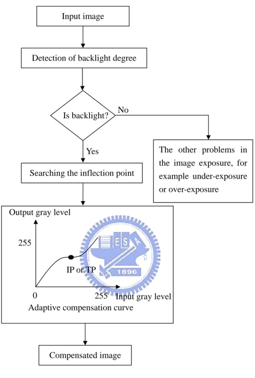
Although the aforementioned techniques can improve the backlight mages to some extend, they usually suffered the problems of over-saturation, losing contrast and so on. Also, there are some articles like [27, 29] proposed using clustering method like fuzzy c-means, neural networks, mass fuzzy rules and pixel-by-pixel compensation algorithm to detect and compensate the backlight images is always required high computation power such that they are not quite suitable for use in the real-time commercial products. In this paper, we propose a new efficient algorithm for detecting and compensating backlight images. The block diagram of the proposed algorithm is shown in Figure 3.1. When taking a photograph, the backlight effect was a result of the main object blocking the primary light source forming insufficient lighting for the main focus object. Therefore, we had to develop a way to enhance the lighting of the main object and retain the color information in the image. In the paper, the input backlight images are initially transformed into the Y. I. Q. color space. In this space, the luminance Y and color information are decoupled, whereY =0.299R+0.587G+0.114B, since luminance is proportional to the amount of light perceived by the human eyes. After the color space transformation, the entire transformed image is analyzed to extract determining features of backlight degree. The analysis is based on the spatial position relation and histogram of images. We will employ fuzzy logic to infer a backlight index to indicate the backlight degree of an image. If the image is not backlighting, it will be processed by the other

auto-exposure methods for solving the possible under-exposure or over-exposure problems and so on. After determining the backlight degree of an image, we will compensate its luminance and keep its contrast according to the estimated backlight degree. To avoid the over-saturation problems, we propose a new adaptive compensation curve scheme for luminance compensation, where the shape of the compensation curve is determined adaptively by its inflection point. Finally, the compensated image is transformed back to the R. G. B. color space from the Y. I. Q. color space defined by:

1 0.956 0.620 1 0.272 0.647 1 1.108 1.705 R Y G I B Q ⎡ ⎤ ⎡ ⎤ ⎡ ⎤ ⎢ ⎥ ⎢_{= − −} ⎥ ⎢ ⎥ ⎢ ⎥ ⎢ ⎥ ⎢ ⎥ ⎢ ⎥ ⎢ − ⎥ ⎢ ⎥ ⎣ ⎦ ⎣ ⎦ ⎣ ⎦ ,

which will restore color information of the compensated image.

The chapter is organized as follows: Section 3.2 describes the proposed backlight detection method, which uses fuzzy inference method to determine the backlight degree of an image. Section 3.4 proposes the backlight compensation method, which utilizes the adaptive cubic curve to compensate the luminance of the backlight image adaptively. Section 3.5 provides and discusses the experimental results. Finally, Section 3.6 gives conclusions and suggestions for the future works.

Figure 3.1 System architecture for detecting and compensating backlight images. Yes

Input image

Is backlight?

Searching the inflection point

Compensated image

The other problems in the image exposure, for example under-exposure or over-exposure

No

0 255

255

Input gray level Output gray level

IP or TP

Adaptive compensation curve Detection of backlight degree

3.2. Backlight Detection Phase

When taking a photograph, the backlight image is a result of the illuminant source behind the main photographic object. Therefore, the brightness of photographed object was displayed with dark brightness, and the luminance difference between the main foreground object and the background was high. In this section, we came up with two indices to detect the backlight degree of an image according to its spatial position characteristics and histogram characteristics, respectively. Fuzzy logic was then used to integrate these two indices into a final backlight index determining the final backlight degree of an image precisely.

(a)

(b)

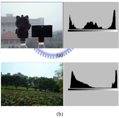
Figure 3.2 Two representative backlight images and their histograms.

To derive the indices for indicating backlight degree of an image, let’s observe two representative backlight images and their histograms shown in Figure 3.2. In Figure 3.2(a), the backlight part is gathering in the central part of the image and there are three groups appearing in the histogram of image. Figure 3.2(b) shows the general

form of backlight images. Its backlight part is also gathering in the central part of the image, but there are only two groups appearing in the histogram of image. No matter the image is which class such as landscape or portrait, the Figure 3.2 shows that an image possibly has different backlight degree.

3.2.1. Backlight Index Based on the Spatial Characteristic of an

Image

The main object usually gathered in the central part of an image when taking a photograph. Furthermore, if the image had backlight problems, the luminance of the main object is low and that of the background was high. Therefore, using the spatial characteristics of an image, we could find the index to represent the backlight degree of the image. To do this, we first used the spatial position segmentation method to divide an image into several sections. Then, according to the strength of area-average luminance, the sections were merged into two areas; one was the background area and the other was main focus object area. The difference of average luminance between the background area and the main object formed an effective index to indicate the backlight degree of the analyzed images.

In the proposed scheme, we divided an image into five areas as shown in Figure 3.3. The photographed object was displayed in the center of image. We left one-fourth part at the top and bottom reserved as background and we left one-forth at the right and left reserved as background for the remaining center area, leaving one half of the whole center area reserve for the main focus object. In the Figure 3.3, the R3 and R5 areas were fixed variables being limited to the main focus object being photographed, and the R1 area was a fixed variable being limited as the true background. The R2 and R4 areas were bi-deviational variables, either as part of the background, referred to as

the first variable, or as part of the main focus object, referred to as the second variable, being photographed. Under the second variable condition, we used the maximum and minimum functions, see below, to determine whether the R2 and R4 areas were used as either the background area or the main-object area by defining the index B_image

below: ), 3 / ] [ 2 / ] ([ 1 24B 3 5 24MO image T MR MR MR MR MR B = + − + + ⎩ ⎨ ⎧ + < = ⎩ ⎨ ⎧ + ≥ = otherwise ), , min( 128 ) and ( if , 2 / ) ( otherwise ), , max( 128 ) and ( if , 2 / ) ( where 4 2 4 2 4 2 24 4 2 4 2 4 2 24 MR MR MR MR MR MR MR MR MR MR MR MR MR MR MO B

where MR being defined as the average value of the gray level of each area _i

and MR_24i was used to determine that region 2 and region 4 were background area, main object area or both are background area or main object area. The T( )⋅ were defined as the membership function which converts B_image into a fuzzy logic degree. The value 20 and 150 were obtained by our experiment. The higher the index value is, the higher the backlight degree of the image is. This index value is obtained from the spatial area and the position of object area and background area in the backlight image.

20 150 1

x T(x)

Figure 3.3 The division of a backlight image.

3.2.2. Backlight Index Based on the Histogram Characteristic of an

Image

In the above section 3.2.1, the B_image index is obtained by averaging the luminance of different spatial areas, including the fixed and deviation variable areas of the image. The probability distribution of image is discussed later in the paper. In this section, we shall derive the B_hist index by indicating the backlight degree of an image based on its histogram Figure 3.4. The Figure 3.4 image shows the representative histogram of a backlight image. This figure illustrates that the backlight image will show the two peak area groupings in the histogram; one group shows a distribution over a low brightness area (T1) and the other group shows a distribution over a high brightness area (T2). Hence, we can separate the histogram into two peak areas according to two threshold values T1 and T2, and one center (gap) area. How did we obtain T1 and T2 values? We employed the Peak Finding Method to achieve this task. The following rules were applied to define the peak points of the histogram.

Step 1: The image histogram was smoothed by the Gaussian smoothing filter. Step 2: The first derivative f’ indicated peak and valley points of the histogram

when the mask -1 1 was convolved with the smoothed histogram. 5 R 4 R 3 R 2 R 1 4h 3 4h 1 4w 3 4w R1

Step 3: The mask -1 1 was re-convolved on step 1 to indicate the second derivative. If the second derivative was less than zero, then first derivative was equal to zero, and the point is at a maximum peak.

Step 4: In step 3, there were many peaks to found. But we had to get a maximum peak value in each group. Hence, according to the property of human vision perception, being that the brightness under 60 gray-level will be regarded as darkness [34], we found a maximum peak value and set it into T1 between 0 and 60. The T2 value was set into the other maximum peak values of greater than 60 gray-level and the maximum gray-level value.

According to these two threshold values, T1 and T2, we can define the second index,B_hist, determining the backlight degree of an image:

2 ( ) 1 B_hist T T p rj j T = ⎛ ⎞ ⎜ _∑ ⎟ ⎜ ⎟ ⎜ ₌ ⎟ ⎝ ⎠ , where p r( )_j nj n

= is the probability of the j gray level, where n was the total th

number of pixels in the image and n was the number of times this level appeared in _j

the image, and T( )⋅ was a membership function which converted B_hist into a fuzzy degree. This index determined the degree of closeness of the two groups in the histogram. When the two clusters were close, the sum of probability of all gray-level between them was very high. This showed that B_hist had a lower value. Thus, the

x 0.5 0 1 0.01 T(x)

analyzed image had a lower backlight degree. On the contrary, higher B_hist value represented a higher backlight degree of the image.

Figure 3.4 The representative histogram of backlight images.

3.2.3. Fuzzy Integration of Two Backlight Indices

In the previous subsections, two indices are derived to indicate the backlight degree of an image based on the average luminance difference of sub-images and the histogram, respectively. Due to the various property and content of backlight images, these two indices have different degrees of reliability. Since the T functions used in the definitions of these two indices convert the indices into fuzzy degrees, we shall apply the fuzzy inference technique to fuse these indices (_Bimage and B

hist) and

produce a more reliable backlight index, B_F, representing the backlight degrees of various kinds of backlight images.

The fuzzy inference rules are characterized by a collection of fuzzy IF-THEN rules in which the preconditions and consequents involve linguistic variables. In the proposed fuzzy inference scheme for backlight detection, there are two input variables,

Bimage and B

hist, and one output variable BF. Each variable has three fuzzy terms

(sets), S (small), M (medium), and B (Big). An identical membership function is used for the fuzzy terms of_Bimage, B_hist and B

F as shown in Figure 3.5, when the

T2

index

. . .

B

h i F of figure is an abbreviation, which can be Bhist, Bimage or BF.

Therefore, nine fuzzy inference rules are used here. Two representative rules are enumerated as follows:

Small Medium Large Small S M M Medium S L M

Large M L L

Figure 3.5 The membership functions of the fuzzy terms of B

hist, Bimage and BF.

Based on the center of area (COA) defuzzification method, we can obtain the

B_F value corresponding to two given _Bimage and B

hist values through fuzzy

inference. The inferred B

F value represents the final estimated backlight degree of

the analyzed image in the detection phase of the proposed scheme. In the next section, this index will be used to find a proper turning point on the adaptive compensation curve in the backlight image compensation phase of our scheme.

. . .

B h i F

0.5

0.2 0.9 Smal Medium Large

Bimage

3.4. Backlight Image Compensation with a Compensation

Curve

3.4.1. The Inspiration

In the previous section, we have mentioned that the characteristic in image histogram of backlight image was that the brightness of main object was darkness and the background brightness was normal. Therefore, we have to adjust main object brightness and keep background brightness.

3.4.2. Compensation Curve Consists of Two Parabolas

In the previous section, we proposed a procedure to detect the backlight degree of an image. After the backlight degree is detected, we can then compensate the backlight image according to the detected backlight degree. In general [26], this is achieved by adding a compensation value to each brightness value of the target image. Although the brightness of the backlight part in the image can be emphasized by this compensation value, the brightness of the background part might be out of the maximum intensity range of image, causing the over-saturation phenomena. To solve this problem, we propose a new image compensation scheme based on adaptive

0 255

255

Input gray level Output gray level

TP

compensation curves. This curve can be automatically adapted to adjust the compensation amount according to the backlight degree of the image. After compensation, the compensated image will keep the characteristics of the original image and the brightness of the backlight part of image will be increased properly.

The proposal compensation curve is shown in the Figure 3.6. It has a turning point, which separates the compensation curve into the upper and lower parts. The lower curve will gradually increase the darkness-part brightness of the input image and the upper curve will keep lightness-part brightness of the input image. By controlling this curve curvature properly, we can compensate the lightness of backlight image successfully without causing the over-saturation problem. To ease the computational complexity, we use parabolic curves to construct the compensation curve. The upper and lower curves are constructed by upward and downward parabolic curves, respectively, which are described by equation (3.1) and (3.2):

( ) ( )2 2 b f x x a b a − = − + (3.1) ( ) (255 )₂( )2 (255 ) b f x x a b a − = − + − , (3.2) where the coordinate of the turning point (i.e., the apex of these two curves) is (a, b), which can be obtained from the estimated backlight degree (B_F) of the image in the backlight detection phase as described in the following procedure.

0 255

255

Input gray level Output gray level

TP

Figure 3.6 Adaptive curve for image compensation.

3.4.3. Compensation Curve Based on Cubic Equation

In section 3.3, we proposed a procedure to detect the backlight degree of an image. After the backlight degree was detected, we could then compensate the backlight image according to the detected degree of backlight. In [27], this was achieved by adding a compensation value to each brightness value of the targeted image. Although the brightness of the backlight area in the image could be enhanced by this compensation value, the brightness of the background area, at times, extended beyond the maximum intensity range of the image, thus, causing the over-saturation phenomena. To solve this problem, we formulated a new image compensation scheme based on adaptive compensation curve. This curve can automatically compensate for the amount of the degree of the backlight of the image. After compensating for the degree of backlight, the compensated image kept the characteristics of the original image and the brightness of the backlight area of image as was enhanced properly.

Subsequently, based on the image processing theory and seeing the results of our experiment, we conclude, that first, the compensation curve can be achieved with the cubic curve equation, and secondly, the domain and co-domain of this curve was between 0 and 255, and thirdly, it shows that some cubic curve characteristics exists. Figure 3.7 (a) and (b) represent the downward concave slope and upward concave slope. Figure 3.7 (c), (d) and (e) represent the various degrees of curve slope. Our compensation curve chose two samples as shown in figure 3.7 (a) and (d). And finally, the maximum and minimum value of the image brightness intensity was the same before and after conversion compensation.

Figure 3.7 (a) Cubic curve with the condition of a>0. (b) Cubic curve with the condition of a<0. (c) Cubic curve with violent curvature. (d) Cubic curve with normal curvature. (e) Cubic curve with over-smooth curvature.

Based on our pre-experiment assumption, the following step by step process concluded our compensated curve assumption was valid. Based on the first assumption, the compensation curve was set as

(3.3) ) ( y= f x =ax3+bx2+cx+d

The compensation curve must pass through points (0, 0) and (255, 255), thus we could determine the value of d, with d being defined as f(0), thus, the curve was simplified as follows: (3.4) ) ( ) 0 ( 2 3 cx bx ax x f y d f + + = = ⇒ = (3.5) 255 ) 255 ( 1 255 255 ) 255 ( 2 2 × − × − = ⇒ + × + × = b a c c b a f

In equation (3.4) the c value was calculated as equation (3.5) and thus, we obtained the following equation:

(3.6) ) 255 ) 255 ( 1 ( ) ( y= f x =ax3+bx2+ −a× 2−b× ×x

Because we wanted to obtain the cubic curve as shown in figure 3.7 (a), the a>0 could satisfy this demand. In order to meet the requirements of the cubic curve in

(b) (a)

figure 3.7 (d), that is the cubic curve function having a horizontal line, the first derivative needed a zero ( f′ x( )=0 ) value. We obtained the following quadratic equation (3.7) 0 2 3 2+ + = c bx ax

According the characteristics of this quadratic equation f′ x( )=0 shows that the quadratic equation had a real root. Hence, the b2− ac4 =0, could satisfy this real root demand. It obtain

(3.8) 3 255 3 ) 255 ( 3 2 2 2 b a a a b = × − × − × × ×

Furthermore, because our compensation curve used a cubic curve, it had an inflection point. The inflection point was ))

3 ( , 3 ( a b f a b − − . Herein, we set (3.9) ) 3 ( and , 3 a b f B a b A=− = − (3.10) 255 0 and 255 0 ≤A≤ ≤B≤

Finally, we substituted (3.9) into equation (3.8) and obtained the following equation: (3.11) 3 255 3 ) 255 ( 1 _{2 2} A A a × + × × − =

We discovered that the compensation curve was related with inflection point in equation (3.11). The following procedure, from steps 1 to 5, was used obtained the compensation curve, shown as the follows:

Step 1: Arbitrarily chosen value of A , whose range was [0, 255].

Step 2: A was given a value in equation (3.11) for solving the value of a. Step 3: When the value aand A were known, they were substituted into

equation (8) to obtain the value of b.

Step 4: When the value of the a and bvariables were known, the value of c was determined.

which is the compensation curve, was obtained.

When we determined what the inflection point was, the cubic curve was obtained immediately. Hence, a proper inflection point can determine any point along the compensation curve and adjust for the effect of backlight image compensation.

3.4.4. Turning Point or Inflection Point Searching

To determine the inflection (or Turning) point, let us observe the histograms of two representative backlight images shown in Figure 3.8 (a) and (b). There are apparently two groups in Figure 3.8 (a). The first group (group A) has lower brightness, and the second group (group B) has higher brightness. We can utilize this characteristic to get the turning point. At first, we calculate the average values of group A and group B, called Lm and Hm, respectively. We use the following steps to

obtain the values of Lm and Hm.

Step 1: Using Gaussian smoothing filter to smooth the histogram of the whole image. Step 2: Calculating a series

{ }

{

}

0 , , ..., , ..., L

j _j j L

a − a a a a ₋

= = and series b by the following equations:

{

}

{

}

where TH is a threshold which is around 0.0013 according to our experimental study. Step 3: According to series a and b to obtain the T set, T =

{

}