軸向滑動梁結構之幾何非線性動態分析

行政院國家科學委員會專題研究計畫 成果報告

軸向滑動梁結構之幾何非線性動態分析

計畫類別： 個別型計畫 計畫編號： NSC93-2211-E-009-026- 執行期間： 93 年 08 月 01 日至 94 年 07 月 31 日 執行單位： 國立交通大學機械工程學系(所) 計畫主持人： 蕭國模 計畫參與人員： 劉宗帆、蔡明旭 報告類型： 精簡報告 處理方式： 本計畫可公開查詢

中 華 民 國 94 年 8 月 24 日

軸向滑動梁結構之幾何非線性動態分析

Geometrically nonlinear dynamic analysis of sliding beam

計畫編號：NSC 93-2211-E-009-026

執行期限：2004 年 08 月 1 日至 2005 年 07 月 31 日

主持人：蕭國模 國立交通大學機械工程學系

計畫參與人員：

劉宗帆、蔡明旭

中文摘要： 本研究的主要目的為提出一簡單有效的共旋轉有限元素法及一數值程序，探討滑動 梁的幾何非線性動態反應。為了正確的描述及預測滑動梁的動態反應，本研究考慮了在 稜柱形導槽內外之梁的運動。在本研究中將梁元素分為二種，第一種是普通梁元素，在 稜柱形導槽外時，該元素的運動不受限制，在稜柱形導槽內時，該元素只能在軸方向運 動。第二種梁元素為本研究提出的一個特別元素，稱為轉接梁元素，該元素有一部分在 稜柱形導槽內，另一部分在稜柱形導槽外。轉接梁元素未變形的長度為一固定長度，但 其在稜柱形導槽內的部分變形前的長度則為時間的函數。本研究在梁元素當前的變形位 置上建立元素座標，並在元素座標上以正確的變形機制推導普通梁元素及轉接梁元素的 節點內力及剛度矩陣。本研究採用基於 Newmark 直接積分法及 Newton-Raphson 法的增 量迭代法求解非線性動態平衡方程式。本研究以數值例題探討滑動梁結構受不同負荷及 端點軸向運動的幾何非線性動態行為並與文獻的結果比較，以說明本研究中提出的方法 的準確性及有效性。 關鍵詞: 滑動梁, 幾何非線性, 共旋轉法, 有限元素法 Abstract.

A simple and effective consistent co-rotational total Lagrangian finite element formulation and a numerical procedure are proposed to investigate the geometric nonlinear dynamic response of sliding beam. To exactly predict the dynamic response of the sliding beam, the total length of the sliding beam is considered. The motion of the beam element is not restrained when it is outside the prismatic joint. The lateral motion of the beam is fully restrained when it is inside the prismatic joint. The beam element is regarded as conventional beam element when it is inside or outside the prismatic joint. The beam element is regarded as transition beam element when it is partially inside the prismatic joint. A transition beam element is developed here. The total undeformed length of the transition element is constant. However, the undeformed length inside the prismatic joint is time dependent. The kinematics, deformations, and equations of motion of the transition beam element are defined in terms of two element coordinate systems constructed at the current configuration of the deformed beam element. The principle of virtual work, d’Alembert principle and the consistent second order linearization of the fully geometrically nonlinear beam theory are used to derive the deformation nodal force and inertia nodal force of the beam element. In element nodal forces, the coupling between bending and stretching deformations of the beam element is considered. An incremental-iterative method based on the Newmark direct integration method and the Newton-Raphson method is employed for the solution of nonlinear dynamic equilibrium equations. Numerical examples are presented to demonstrate the accuracy and efficiency of the proposed method.

Keywords: Sliding Beam, Geometrical Nonlinearity, Co-rotational Formulation, Finite Element Method

1 INTRODUCTION

In recent years, the dynamic behavior of flexible sliding beam with prismatic joint, e.g. robotic manipulators, spacecraft antenna and deployable space structures, has been the subject of considerable research [1-5]. Currently, the most popular approach for the analysis of beam structures is to develop finite element models. However, not many finite element formulations for sliding beams have been reported in the literature. Moreover, the geometrically nonlinear finite element formulations for sliding beam reported [4, 5] are very complicated.

The objective of the paper is to propose a simple and effective consistent co-rotational total Lagrangian finite element formulation and a numerical procedure for the geometrically nonlinear dynamic analysis of sliding beam. When the beam element is inside or outside the prismatic joint, the beam element proposed in [6] is adapted and used and is called conventional beam element here. A transition beam element is developed here when the beam element is partially inside the prismatic joint. The total undeformed length of the beam element is constant. However, the undeformed length inside the prismatic joint for the transition beam element is time dependent. The kinematics, deformations, and equations of motion of the transition beam element are defined in terms of two element coordinate systems constructed at the current configuration of the deformed beam element. The principle of virtual work, d’Alembert principle and the consistent second order linearization of the fully geometrically nonlinear beam theory are used to derive the deformation nodal force and inertia nodal force of the beam element. An incremental-iterative method based on the Newmark direct integration method and the Newton-Raphson method is employed for the solution of nonlinear dynamic equilibrium equations. Numerical examples are presented to demonstrate the accuracy and efficiency of the proposed method.

2 FINITE ELEMENT FORMULATION 2.1 Description of problem

Consider a uniform Euler beam with prismatic joint, which slides through the prismatic joint fixed in space at a prescribed end displacement U_A(t) as shown in Fig. 1. The beam element is regarded as a conventional beam element when it is inside or outside the prismatic joint, and regarded as a transition beam element when it is partially inside the prismatic joint. The beam element proposed in [6] is adapted and used as the conventional beam element here. A transition beam element is developed here. The transition element is divided into two segments. The segments inside and outside the prismatic joint are called the first segment and the second segment of the transition element, respectively. The displacement and slope are continuous at the intersection of the two segments. The total undeformed length of the beam element is constant. However, the undeformed length of the first segment and the second segment of the transition element are time dependent.

2.2 Basic assumptions

The following assumptions are made in derivation of the beam element behavior. 1. The beam is uniform and slender, and the Euler-Bernoulli hypothesis is valid. 2. The unit extension of the centroid axis of the beam element is uniform. 3. The deformation displacements and rotations of the beam element are small. 4. The strains of the beam element are small.

1 2 3 1 u 3 v 3 u 3 u 2 u 2 v 1 l 2 l 3 φ 2 φ 1 x 2 x 1 x 2 x C

Figure 1: Sliding beam.

2.3 Coordinate systems

In this paper, a co-rotational total Lagrangian formulation is adopted. In order to describe the system, we define two sets of coordinate systems:

A fixed global set of coordinates, X (i = 1, 2) (see Fig. 1); the nodal coordinates, nodal _i

displacements and rotations, velocities, accelerations, and the equations of motion of the system are defined in this coordinates.

Element coordinates; x , _i x (i = 1, 2) (see Figs. 2, 3), a set of element coordinates is _i

associated with each conventional element and each segment of the transition element, which is constructed at the current configuration of the beam element.

Figure 2: Element coordinates and kinematics Figure 3: Element coordinates for the for the conventional beam element transition beam element

) (t U_A L A B 1 X 2 X C Beam Sliding Deformed Joint Prismatic Beam Sliding Undeformed 1 2 x 1 x y x P Q 1 P Q y 1 x 2 x s ) (x v ) (x x_p φ x1S S x₂

2.4 Conventional beam element

The beam element proposed in [6] is adapted and employed here. In the following only a brief description is given.

The geometry of the beam element is described in the current element coordinate system. Let Q (Fig. 2) be an arbitrary point in the beam element, and P be the point corresponding to

Q on the centroid axis. The position vector of point Q in the undeformed and deformed

configurations may be expressed as

2 1 0 e e r =x +y (1) and 1 ] sin ) , ( [ e r= x_p x t −y φ +[v(x,t)+ ycosφ]e₂ (2) o v s x x v s v ε φ + ′ = ∂ ∂ ∂ ∂ = ∂ ∂ = 1 sin ₍₃₎ 1 − ∂ ∂ = x s o ε (4)

where x_p( tx, ), v( tx, ) are the x₁, x₂ coordinates of point P referred to the current element coordinates, respectively, in the deformed configuration, φ =φ( tx, ) is the angle measured from x₁ axis to centroid axis of the beam element, and e (i = 1, 2) denote the _i unit vectors associated with the x axis. _i ε_o is the unit extension of the centroid axis and s is the arc length of the deformed centroid axis measured from node 1 to point P. In this paper, the symbol ( ′ denotes ) ()_,x =∂() ∂x.

The relationship between x_p( tx, ), v( tx, ) in Eq. (2) may be given as

dx v u t x x_p = +

∫

x + _o − _x 0 2 1 2 , 2 1 [(1 ) ] ) , ( ε (5)

where u₁ is the displacement of node 1 in the x₁ direction. Note that due to the definition of the element coordinate system, the value of u₁ is equal to zero. However, the variations and time derivatives of u₁ are not zero. Making use of Eq. (5), one obtains

) , 0 ( ) , ( 1 2 u x Lt x t u L+ − = _p − _p = l =

∫

L + _o −v_x dx 0 2 1 2 , 2 _] ) 1 [( ε (6)

in which _l is the current chord length of the centroid axis of the beam element, and L is the length of the undeformed beam axis, and u₂ is the displacement of node 2 in the x₁

direction.

Making use of the assumption of uniform unit extension and retaining all terms up to the second order in Eq. (6), one may obtain

∫

+ − = Lv_xdx L L L 0 2 , 0 2 1 l ε (7)

polynomials of x, and may be expressed by b t b t v v v v N N N N t x v( , )={ ₁, ₂, ₃, ₄} {₁, ₁′, ₂, ′₂}=N u (8) ) 2 ( ) 1 ( 4 1 2 1= −ξ +ξ N , (1 )(1 ) 8 2 2 = −ξ −ξ L N (1 ) (2 ) 4 1 ₂ 3= +ξ −ξ N , ( 1 )(1 ) 8 2 4= − +ξ +ξ L N , L x 2 1+ − = ξ (9)

where v_j (j = 1, 2) are nodal values of v at nodes j, respectively, v′_j (j = 1, 2) are nodal values of v_,x at nodes j, respectively. Note that, due to the definition of the element coordinates, the values of v_j (j = 1, 2) are zero. However, their variations and time derivatives are not zero. In this paper, { } denotes column matrix.

If x and y in Eq. (1) are regarded as the Lagrange coordinates, the Green strain ε and the ₁₁ corresponding engineering strain e₁₁ is given by [7]

) 1 ( 2 1 , , 11 = rtxrx − ε (10) 2 1 11 11=(1+2ε ) e (11)

Substituting Eqs. (2-4) and (10) into Eq. (11) and retaining all terms up to the second order yield

xx yv

e₁₁=ε₀+(1−ε₀) _, (12) The element nodal force vector is obtained from the d’Alembert principle and the virtual work principle in the current element coordinates. The virtual work principle requires that

= = + = t _{b int} b a t a ext W W δ δ δ δ u f uφ f

∫

+ V t t dV e ) (δ ₁₁σ₁₁ ρδr &&r (13) } , { u₁ u₂ a δ δ δu = , δuφ_b ={δv₁,δφ₁,δv₂,δφ₂} (14) f_a f_ad f ai f f = + = { ₁₁, ₁₂}, f_b =f_bd +f_bi ={f₂₁,m₁, f₂₂,m₂} (15) where f_j (j = a, b) denotes the internal nodal force vector corresponding to δu_a, δuφ_b,

f_jd_{and f} j i

(j = a, b) are the deformation nodal force vectors and the inertia nodal force vectors, respectively, V is the volume of the undeformed beam element, δe₁₁ is the variation of e₁₁ in Eq. (12) with respect to the nodal parameters, σ₁₁=Ee₁₁ is the normal stress, where E is Young’s modulus, ρ is the density, rδ is the variation of r given in Eq. (2) with respect to the nodal parameters, and r&&=∂2r/ t∂ 2. In this paper, the symbol (•) denotes time derivative ∂ /() ∂t. φ_i(i = 1, 2) are the nodal value of φ defined in Eq. (3) at nodes i.

Substituting Eqs. (2), (7)and (8) into Eq. (13), and using consistent linearization, f_jdand f_ji (j = a, b) may be given by a d a AEL G f = ε₀ (16) dx v EI dx v EA _{b x b xx} d b = 0

∫

N′ , +

∫

N′′ , f ε (17) dx dx v dx v L x A dx A _a t_{a a a} L _x x _x i

a =

∫

N N u&& +

∫

N (

∫

₀ &,2 −

∫

₀&,2 )

f ρ ρ (18) dx v I dx v I dx v A _{b b x} t_{a a b x} i

b =

∫

N && +

∫

N′ &&, −2 G u&

∫

N′ &,

f ρ ρ ρ (19) } 1 , 1 { 1 − = L a G , } 2 1 , 2 1 { −ξ +ξ = a N (20)

where A is the cross-section area and =

∫

Ay dA

I 2 . The range of integration for the integral

∫

()dxin Eqs. (17)-(19) is from 0 to L.

The element stiffness matrix and inertia matrix may be obtained by differentiating the element nodal force vectors f_j (j = a, b) in Eqs. (15) with respect to the nodal parameters and their time derivatives. The element stiffness matrices and consistent mass matrices of the beam element may be given by

Stiffness matrices: t a a a AELG G k = , k_b =k₀+k_g =EI

∫

N_b′′N_b′′tdx+AEε₀

∫

N′_bN_b′tdx (21) Mass matrices: dx A _a t_a a N N m =ρ

∫

, m_b =ρA

∫

N_bNt_bdx+ρA

∫

N′_bN′_btdx (22) where the range of integration for the integral

∫

()dxin Eqs. (21)-(22) is from 0 to L.

Note that the element coordinate system is only a local coordinate system not a moving coordinate system here. Thus the element matrices referred to the global coordinate system may be obtained from Eqs. (21-22) by using the standard coordinate transformation.

2.5 Transition beam element

The beam element is regarded as a transition beam element when it is partially inside the prismatic joint. A transition beam element is developed here. In the following the derivation of the transition beam element is given.

The geometry of the first and the second segments of the transition beam element is described in the current element coordinate systems x and x_{i i}(i = 1, 2), respectively as shown in Fig. 3. Let C be the end point of the prismatic joint, and node 3 be the intersection

of the first and the second segments of the transition beam element. However, the displacement and slope at node 3 are continuous. Thus, the tangent of node 3 is in the x₁

direction and node 3 can move in the x_{1 direction only. Because the displacement and}

virtual displacement of node 3 can be determined from the positions and virtual displacements of nodes 1 and 2, and the assumption of the uniform unit extension of the beam element, node 3 is not an independent node. The transition beam element developed here has two independent nodes – nodes 1 and 2, and four degree of freedoms - u₁, u₂, v₂, and φ₂ as shown in Fig. 3. Let L₁ and L₂ denote the length of the first and second segments in the undeformed state. Note that L₁ and L₂are functions of time. However, their sum is a constant and may be expressed by

L L

L₁+ ₂ = (23)

where L is the total length of the undeformed beam element.

When the positions and of nodes 1 and 2, and the value of φ₂are determined, _l1 and _l2, the current chord length of the first and second segment, and φ₃, the deformation rotation of node 3, can be calculated.

Making use of the assumption of uniform unit extension and Eq. (7), one may obtain 1 1 2 2 1 1 0 = − = + v− L L ε ε l l ₍₂₄₎

∫

= 2 0 2 , 2 2 1 L x v v dx L ε ₍₂₅₎

From Eqs. (23) and (24), one may obtain ) 1 ( 2 2 1 1 v L L L ε l l l l ₋ = , (1 ) 2 1 2 2 v L L L ε l l l l ₊ = ₍₂₆₎ 1 2 0= + v− L ε ε l l l , l=l₁+l₂ (27)

The position vector of an arbitrary point in the undeformed and deformed configurations of the first segment may be expressed as

2 1 0 e e r =x +y , 0≤x≤L₁ (28) and 2 1 0 1 (1 ) ] [ e e r= u + +ε x +y (29) wheree ( i = 1, 2 ) are unit vectors associated with the _i x axis，_i u₁ is the displacement of node 1 in the x₁ direction. ε₀ is given in Eq. (27). Note that due to the definition of the element coordinate system, the value of u₁ is equal to zero. However, the variations and time derivatives of u₁ are not zero.

Let u denote the displacement of node 3 in the ₃ x₁ direction. From Eqs. (28) and (29), one may obtain

1 0 1

3 u L

u = +ε (30) From Eqs. (27) and (30), the variation of u may be expressed by ₃

) ( _{2 1} 1 1 3 u u L L u u δ δ δ δ = + − (31)

The position vector of an arbitrary point in the undeformed and deformed configurations of the second segment may be expressed as

2 1 0 e e r =x +y , 0≤x≤L₂ (32) and 1 ] sin ) , ( [ e r= x_p x t −y φ +[v(x,t)+ycosφ]e_{2 (33)} dx v u t x x_p = +

∫

x + _o − _x 0 2 1 2 , 2 3 [(1 ) ] ) , ( ε (34)

where u is the displacement of node 3 in the x_{3 1} direction. v( tx, ), φ is the angle measured from x₁ axis to centroid axis of the beam element, and e (i = 1, 2) denote the _i unit vectors associated with the x axis. Note that due to the definition of the element _i

coordinate system, the value of u and ₃ v is equal to zero, where ₃ v is the displacement ₃

of node 3 in the x₂ direction. However, their variations and time derivatives are not zero. From the continuity of the displacement and slope at node 3 and Fig. 3, one may obtain

3 3 3 δ cosφ

δu = u , δv₃=δu₃sinφ₃ (35)

Here, the lateral deflections of the centroid axis, v( tx, )is assumed to be the Hermitian polynomials of x, and may be expressed by

b t b t v v v v N N N N t x v( , )={ ₁, ₂, ₃, ₄}{ ₃, ₃′, ₂, ′₂}=N u (36) ) 2 ( ) 1 ( 4 1 ₂ 1= −ξ +ξ N , (1 )(1 ) 8 2 2 2 = −ξ −ξ L N (1 ) (2 ) 4 1 ₂ 3= +ξ −ξ N , ( 1 )(1 ) 8 2 2 4 = − +ξ +ξ L N , 2 2 1 L x + − = ξ ₍₃₇₎

where v_j (j = 2, 3) are nodal values of v at nodes j, respectively, v′_j (j = 2, 3) are nodal values of v_,x at nodes j, respectively. Note that the variations and time derivatives of the shape functions should be considered for the second segment.

From Eqs. (3), (4) (29), (33), (10) and (11) and retaining all terms up to the second order, one may obtain

0 11 =ε e , 0≤x≤L₁ (38) and xx yv e₁₁=ε₀ +(1−ε₀) _, , 0≤x≤L_{2 (39)}

The derivation of the element nodal force for the transition element is similar to that for the conventional beam element and given as follows:

The virtual work principle requires that

= = + = t _{b int} b a t a ext W W δ δ δ δ u f uφ f

∫

+ V t t dV e ) (δ ₁₁σ₁₁ ρδr &&r (40) } , { u₁ u₂ a δ δ δu = , δuφ_b ={δv₂,δφ₂} (41) } , {f₁₁ f₁₂ i a d a a =f +f = f , f_b =f_bd +f_bi ={f₂₂,m₂} (42) where f_j (j = a, b) denotes the internal nodal force vector corresponding to δu_a, δuφ_b,

f_jd_{and f} j

i_{(j = a, b) are the deformation nodal force vectors and the inertia nodal force}

vectors, respectively, V is the volume of the undeformed beam element. δe₁₁ is the variation of e₁₁ in Eqs. (38) and (39) with respect to the nodal parameters for segment 1 and segment 2, respectively.

Substituting Eqs. (29)-(31), (33), (35)-(36), (38) and (39) into Eq. (40), and using consistent linearization, f_jdand fi_j(j = a, b) may be given by

a d a AEL G f =

ε

₀ (43) dx v EI dx v EA L _{b x} L _{b xx} d b 0 ₀ 2 , ₀ 2 , 2 2

∫

∫

′ + ′′ = N N f ε (44)

∫

∫

∫

+ = L t _a L _a L _x a a i a v dx dx L x A dx A 0 0 2 , 0 ( ) 2 & && N u N N f ρ ρ (45) dx dx v L x L L x L A L ({1 , } x _x ) 0 2 , 1 1 0 2

∫

∫

− + + −ρ _&

∫

∫

∫

+ ′ − ′ = 2 2 2 0 2 , 0 2 , 0 2 2 L x b a t a L xx b L b i

b A N v&&dx I N v&& dx IG u& N v& dx

f ρ ρ ρ (46) } , { _{3 4} 2 N N b = N (47)

where G and _a N are defined in Eqs. (20), respectively, _a N and ₃ N₄ are defined in Eq. (37).

The element stiffness matrix and inertia matrix may be obtained by differentiating the element nodal force vector f_j (j = a, b) in Eqs. (42) with respect to the nodal parameters and

their time derivatives. The element stiffness matrices and consistent mass matrices of the transition beam element may be given by

Stiffness matrices: t a a a AELG G k = , = + =

∫

2 ′′ ′′ +

∫

2 ′ ′ 0 2 2 0 0 2 2 0 L _t b b L _t b b g b k k EI N N dx AE N N dx k ε (48) Mass matrices:

∫

= L t a a a A ₀N N dx m ρ , =

∫

2 +

∫

2 ′ ′ 0 2 2 0 2 2 L _t b b L _t b b b A N N dx A N N dx m ρ ρ (49)

2.6 Element damping force vector

Here the proportional damping is considered. The element damping force vector may be expressed by [8] j j v j c u f = _& (50) j j j m k c =α +β ₍₅₁₎

where j = a, b, c_j is the so called damping matrix, u&_j is the element nodal velocity,

j

m and k_j are the corresponding mass and stiffness matrix, respectively for the conventional and the transition beam element. Note that only k is considered for ₀ k _b given in Eqs. (21) and (48). α and β are the so called damping coefficients.

2.7 Equations of Motion

The nonlinear equations of motion may be expressed by 0 P F F F Ψ= I + D+ V − = ₍₅₂₎ where Ψ is the unbalanced force among the inertia nodal force FI, deformation nodal force

F

D, damping nodal force

F

V, and the external nodal force P.

In this paper, an weighted Euclidean norm of the unbalanced force is employed for the equilibrium iterations, and is given by

tol

e N ≤

Ψ

(53) where N is number of the equations of the system; e_tol is a prescribed value of error tolerance.

3 NUMERICAL EXAMPLES

An incremental iterative method based on the Newmark direct integration method [6, 9] and the Newton-Raphson method is employed here. The procedure proposed in [9] to determine the nodal deformation rotation for individual elements is employed here.

Let L and L denote the total length of the sliding beam and the initial length of the ₀

sliding beam outside the prismatic joint, respectively. The prescribed end displacement )

(t

U_A of the sliding beam considered here has two different types and may be expressed as 2 0 0 2 1 ) (t v t a t U_A = + (54) and ⎪⎩ ⎪ ⎨ ⎧ > ≤ − = 0 0 0 0 0 0 0 ), ( ), 2 sin 2 ( ) ( t t t U t t t t t t t c t U A A π π (55)

where v , ₀ a , ₀ c , and ₀ t are constants. ₀

To obtain the damping coefficients in Eq. (51), the modal damping functions used in [3, 5] are used here and given by

1 2 0 1 )] ( [ 4 4874 . 0 ω ξ t U L + _A = , 2 2 0 2 )] ( [ 4 124 . 3 ω ξ t U L + _A = ₍₅₆₎

where L is the initial length of the sliding beam outside the prismatic joint, ₀ ω_i is the ith natural frequencies of a cantilever beam of length L₀+U_A(t).

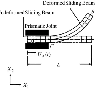
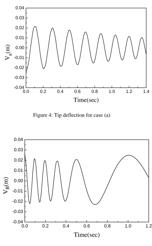
The geometry and material properties of the sliding beam used here are [3, 5]: cross section area A=4.3434×10−5m2, area moment of inertia I =1.059×10−11m4, Young's modulus E=68.96×109N/m2 , and the density ρ =3144.3858kg/m3. Four cases are considered: (a) L=0.762m , L₀ =0.521m , v₀ =−0.03m/s , a₀=−0.054m/s2 (b)

m

L=1.05 , L₀ =0.35m, c₀ =0.7m, t₀ =1.2s

For all cases, the sliding beam is initially at rest, and the magnitude of the initial lateral tip deflection is 0.024 m, which is induced by the application of a lateral force at the free end of the beam. Note that the lateral force is removed when t > 0. The beam initially inside and outside the prismatic joint is discretized by 14 and 10 equal element, respectively. The time step sizes are chosen to be 0.001 sec. The time history of the tip displacements are shown in Figs. 4-5. The agreement between the present results, the experimental results reported by [3] (not shown) and the results of linear analysis [3, 5] (not shown) is very good. The nonlinear solution reported by [5] exhibits period elongation relative to the linear solution and shows higher amplitudes. Thus, the nonlinear solution reported by [5] might be incorrect.

0.0 0.2 0.4 0.6 0.8 1.0 1.2 1.4 -0.04 -0.03 -0.02 -0.01 0.00 0.01 0.02 0.03 0.04

V

B

(m

)

Time(sec)

Figure 4: Tip deflection for case (a)

0.0 0.2 0.4 0.6 0.8 1.0 1.2 -0.04 -0.03 -0.02 -0.01 0.00 0.01 0.02 0.03 0.04

V

B

(m

)

Time(sec)

Figure 5: Tip deflection for case (b)

4 CONCLUSIONS

A simple and effective consistent co-rotational total Lagrangian finite element formulation and a numerical procedure are proposed to investigate the geometric nonlinear dynamic response of sliding beam.

beam is considered. The beam element is regarded as a conventional beam element when it is inside or outside the prismatic joint, and regarded as a transition beam element when it is partially inside the prismatic joint. The beam element proposed in [6] is adapted and used as the conventional beam element here. A transition beam element is developed here. The total undeformed length of the beam element is constant. However, the undeformed length of the first segment and the second segment of the transition element are time dependent. The kinematics, deformations, and equations of motion of the transition beam element are defined in terms of two element coordinate systems constructed at the current configuration of the deformed beam element. The principle of virtual work, d’Alembert principle and the consistent second order linearization of the fully geometrically nonlinear beam theory are used to derive the deformation nodal force and inertia nodal force of the beam element.

An incremental-iterative method based on the Newmark direct integration method and the Newton-Raphson method is employed for the solution of nonlinear dynamic equilibrium equations. From the numerical examples studied, the accuracy and efficiency of the proposed method is well demonstrated..

REFERENCES

[1] C.D. Jr. Mote. Dynamic stability of axial moving material. Shock Vibration Dig., U. S. Naval Research Laboratory, 4, 2-11, 1972.

[2] J.A. Wickert and C.D. Mote. Current research on the vibration and stability of axially-moving materials. The Shock and Vibration Digest, 20, 3-13, 1988.

[3] J. Yuh and T. Young. Dynamic modeling of an axially moving beam in rotation: simulation and experiment. ASME J. Dyn. Systems Measurements Control, 113, 34-40, 1991.

[4] L. Vu-Quoc and S Li. Dynamics of sliding geometrically-exact beams: large angle maneuver and parametric resonance. Comput. Meth. Appl. Mech. Engng., 120, 65-118, 1995.

[5] K. Behdinan and B. Tabarrok. A finite element formulation for sliding beams, Part I. Int.

J. Numer. Meth. Engng., 43, 1309-1333, 1998. Part II : time integration. Int. J. Numer. Meth. Engng., 43, 1335-1363, 1998.

[6] K.M. Hsiao, R.T. Yang and A.C. Lee. A consistent finite element formulation for non-linear dynamic analysis of planar beam. Int. J. Numer. Meth. Engng., 37, 75-89, 1994.

[7] T.J. Chung. Continuous Mechanics. Prentice-Hall, Inc., Englewood Cliff, New Jersey, 1988.

[8] S.S. Rao. Mechanical Vibrations, Third Edition. Addision-Wesley, 1995.

[9] K.M. Hsiao and J.Y. Jang. Nonlinear Dynamic Analysis of Elastic Frames. Comput.