Maximum Trimmed Likelihood Estimator for
Multivariate Mixed Continuous and Categorical Data
Tsung-Chi Cheng
∗November 30, 2006
Abstract
In this article we apply the maximum trimmed likelihood (MTL) approach (Hadi
and Luce˜no 1997) to obtain the robust estimators of multivariate location and shape,
especially for data mixed with continuous and categorical variables. The forward search algorithm (Atkinson 1994) is adapted to compute the proposed MTL estimates. A simulation study shows that the proposed estimator outperforms the classical maximum likelihood estimator when outliers exist in data. Real datasets are also used to illustrate the method and results of the detection of the outliers.
Keywords: Maximum trimmed likelihood estimator, minimum covariance determinant
estimator, mixture data, Mahalanobis distance, multiple outliers, robust diagnostics.
1
Introduction
The detection of multiple outliers in multivariate data has been a particularly intractable problem. There is a number of approaches for their identification, which essentially requires a robust estimation of multivariate location and shape. A difficulty is that most estimation procedures are known to break down when the fraction of contamination is greater than 1/(p + 1), where p is the dimension of the data. Both the minimum volume ellipsoid (MVE) and the minimum covariance determinant (MCD) estimators provide a high breakdown of the robust estimation of multivariate location and shape (Rousseeuw and Leroy 1987). Moreover, Butler et al. (1993) show that the MCD estimator has better theoretical properties than the MVE. Woodruff and Rocke (1994) give empirical results which show that the MCD is
∗Department of Statistics, National Chengchi University, 64 ZhihNan Road, Section 2, Taipei 11605,
preferred over the MVE in their applications. Croux and Haesbroeck (1999) discuss other statistical properties of robustness about MCD.
Ever since the last decade of the twentieth century, one of the most important research topics about robust statistics has focused on exploring the fast and efficient algorithms to obtain the existing robust estimates. Hawkins (1994) presents a feasible solution algorithm for the MCD which involves taking random starting “trial solutions” and refining each to a local optimum satisfying the necessary condition for the MCD criterion. Rocke and Woodruff (1996) propose a hybrid algorithm using the MCD as the first-stage estimate. They pay at-tention to high dimensional problems (up to 40) and also compare a variety of algorithms. Rocke and Woodruff (1997) describe an overall strategy for the robust estimation of mul-tivariate location and shape, which involves a variety of recent methods. Atkinson (1994) proposes the forward search algorithm, which not only rapidly finds estimates satisfying the criterion but it also leads to the detection of multiple outliers. Rousseeuw and van Driessen (1999) propose a fast procedure for MCD, which is available in S-PLUS and some other sta-tistical computing packages. They show that after starting any approximation to the MCD estimate, it is possible to obtain another approximation yielding an even lower objective function. They call this a C-step, where C stands for “concentration”.
Rather than directly trimming the data, Hadi and Luce˜no (1997) present the trimmed likelihood estimator, which is based on trimming the likelihood function. They refer to this method as the maximum trimmed likelihood (MTL) method and the corresponding estimator as the maximum trimmed likelihood estimator (MTLE). M¨uller and Neykov (2003) discuss the relationships of the least trimmed squares (LTS) estimator and MTLE for a generalized linear model. Cheng (2005) combines both robust and diagnostic approaches to obtain the robust regression transformation, in which LTS and MTLE are also linked together.
Most robust estimations focus on the data only with continuous variables. There are relatively few works available about robustness and outliers under a categorical data analysis (e.g. Bartlett and Lewis (1994), Basu and Basu (1998), Shane and Simonoff (2001)). For the linear regression problem, previous studies consider the case where both response and regressors are continuous. In practice, quite often the data are mixed with both continuous and categorical regressor variables. However, a problem of singularity may occur when directly applying those robust estimators to a model of this kind. Until quite recently, a couple of papers solve the difficulty by separating the continuous and discrete regressors (see Hubert and Rousseeuw (1997), and Maronna and Yohai (2000)). The problem of singularity occurs as well for those robust estimators when applied to multivariate data with a mixture of continuous and categorical variables.
In the statistical literature, researchers have paid much attention to the estimation of a statistical distance between populations, where continuous and discrete variables are com-bined (eg. Krzanowski (1983), Bar-Hen and Daudin (1995), Bedrick et al. (2000), and de Leon and Carri´ere (2005)). All are based on the likelihood approach, which requires cal-culating the maximum likelihood estimates (MLE) of mean vectors and covariance matrix. However, multiple outliers may have a strong effect on MLE and hence influence the estimate of the distance. In this article we apply the forward search algorithm to the MTL approach, from which we are able to obtain the robust estimation of multivariate location and shape, especially for mixed data, and outliers can be revealled as well.
The paper is outlined as follows. We first discuss some issues related to the MCD in Sec-tion 2. The idea of the trimmed likelihood approach is connected with MCD for multivariate data. Section 3 first shows the general location model for mixture data and then extends the MTLE to data of this kind. The forward search algorithm is extended for the resulting estimator. A small scale simulation study is carried out to compare the performance of MLE and MTLE when different proportions of outliers exist in data. Section 4 illustrates the proposed procedure using two real data examples. Section 5 concludes.
2
The MCD estimator and related problems
The definition of the MCD is presented in this section. We then build up its relationship with the trimmed likelihood estimator.
2.1
The MCD estimator
Let yT
i be the ith of n observations on a p-variate normal population, and Q ∈ Q is an
arbitrary subset of {1, 2, · · · , n} of size q = [nγ], 0 < γ < 1, where q is referred to as the quantile index. We denote the sample mean and covariance matrix based on this subset by ¯
y(Q) and S(Q), respectively, as:
¯ y(Q) = 1 q X i∈Q yi, S(Q) = 1 q − 1 X i∈Q (yi− ¯y(Q))T(yi− ¯y(Q)),
where ¯y(Q) is a p × 1 vector and S(Q) is a p × p matrix.
Consider the subset ˆQ of {1, 2, · · · , n} for which the determinant of S(Q), |S(Q)|, attains
the q points for which the classical tolerance ellipsoid has minimum volume and then taking its center as the estimator of the mean. We call (¯yq, Sq) = (¯y( ˆQ), S( ˆQ)) the minimum
covari-ance determinant (MCD) estimator. It is affinely equivariant and its empirical distribution
converges at the rate of n−1/2, whereas the convergence rate of the MVE is n−1/3 (Butler et
al. 1993). Butler et al. (1993) also find the consistency and asymptotic normality for the
MCD estimator of multivariate location and the consistency for that of multivariate shape. One practical issue is that the MCD requires a decision on q. This means that one needs to decide how many observations h are to be trimmed. Hawkins (1994) suggests two possible approaches. One is to use the value of h that provides the maximum breakdown point and so accommodates the maximum possible number of potential outliers. The maximizing h is (Rousseeuw and Leroy 1987, p. 264)
h∗ = n −
·n + p + 1
2
¸
,
where [·] indicates the integer part. The other approach is to trim some smaller number of cases in the quite common anticipation that no more than a few cases might be outliers. Zaman et al. (2001) suggest that [0.75n] is a reasonable value for q for applying LTS in most empirical studies. This suggestion should also be reasonable for MCD.
2.2
The maximum trimmed likelihood estimator
Hadi and Luce˜no (1997) propose a trimmed likelihood principle based on trimming the likelihood function rather than directly trimming the data. They show that this trimming likelihood principle produces many existing estimators, such as MLE, least median of squares (LMS), LTS, and MVE. It is always possible to order and trim observations according to their contributions to the likelihood function, because the likelihood is scalar-valued. For any given value of θ,
l(θ; x1) ≥ l(θ; x2) ≥ · · · ≥ l(θ; xn),
where l(θ; xi) = ln f (xi; θ) is the contribution of the ith observation to the log likelihood
function. Therefore, the ML estimator maximizes the log likelihood function as
n
X
i=1
l(θ; xi).
The method proposed by Hadi and Luce˜no (1997) replaces the log likelihood function by the trimmed log likelihood function:
b
X
i=a
where a ≤ b, (a, b) ∈ {1, 2, · · · , n}, and wi ≥ 0 are weights. The estimator θ(a, b, w) is
obtained by maximizing (??). They call this method as the maximum trimmed likelihood
(MTL) method and ˆθ(a, b, w) is the maximum trimmed likelihood estimator (MTLE).
Consider the case of wi = 1, a ≤ i ≤ b. When a = 1 and b = n, ˆθ(1, n) is the MLE
of θ, so that MLE is a special case of MTLE. When a = b = [n+1
2 ], the resulting estimator
is the maximum median likelihood estimator (MMLE). For multivariate normal data, the MMLEs of µ and Σ are the same as the MVE estimates of µ and Σ (Theorem 5.1 of Hadi and Luce˜no (1997)).
We now show that when a = 1 and b = q, the MCD is also the MTLE of θ = (µ, Σ).
Consider the density function of yT
i : f (yT i , θ) = Ã 1 √ 2π !p |Σ|−1/2exp ½ −1 2(yi− µ) TΣ−1(y i− µ) ¾ , and li = l(θ, yiT) ˙= − 1 2log |Σ| − 1 2d 2 i, (2) where d2
i = (yi− µ)TΣ−1(yi− µ) is the squared Mahalanobis distance. The estimate of the
squared Mahalanobis distance for the ith observation is
d2
i = (yi− ¯y)TS−1(yi− ¯y),
where ¯y and S denote the MLE of the mean vector and covariance matrix, respectively.
Asymptotically, d2
i follows a chi-squared distribution with p degrees of freedom. The larger
values of d2
i can be used to flag the outlying observations in data. However, the effect of
outliers on the estimates ¯y and S leads to the rapid breakdown of the Mahalanobis distances
for the detection of outliers.
From (??), we see that the greater the value of d2
i is, the smaller the value of li will be.
This also implies that we can use li as well as d2i to order the observations. If Q indicates
the subset that corresponds to those q observations yielding the desired robust estimates (ˆµq, ˆΣq) of the trimmed likelihood
q X i=1 l(θ; yT i ) = − q 2log |Σq| − q 2 q X i=1 d2 i,
then this implies
sup Q∈Q q X i=1 li = − q 2log | ˆΣq| − q 2 X i∈Q d2 i. (3)
Here, ˆθ(1, q) = (ˆµq, ˆΣq) denotes the MTLE of the mean vector and covariance matrix, which are ˆ µq = X i∈Q yi ˆ Σq = 1 q − 1 X i∈Q (yi− ˆµq)T(yi− ˆµq),
respectively. The squared robust Mahalanobis distance for observation i is
d2
iq = (yi− ˆµq)TΣˆ −1
q (yi− ˆµq), i = 1 · · · n. (4)
As ˆθ(1, q) = (ˆµq, ˆΣq) is the MLE of the subset Q,
X
i∈Q
(yi− ˆµq)TΣˆ −1
q (yi− ˆµq) = (q − 1)p.
Thus equation (??) reduces to max q X i=1 li ≡ inf Q∈Q|Σ(Q)| = |Σ( ˆQ)| ≡ | ˆΣq|, which is the MCD.
2.3
The forward search algorithm
The forward search algorithm starts with a randomly selected subset of observations. The observations of the subset are incremented in such a way that outliers are unlikely to be included. The algorithm can be briefly summarized as follows.
• (F0) Choose m observations (e.g. m = p + 1, the so-called elemental set) from the
dataset.
• (F1) Obtain the ML estimates based on the subset, compute the squared Mahalanobis
distances for all observations, and order the distances.
• (F2) Calculate the value of the objective criterion, such as MVE and MCD.
• (F3) Choose m + s (usually s = 1) cases with the smallest squared distances of (F1)
as the new subset, and return to step (F1).
We call steps (F0) to (F4) a one forward search. There are two ways for obtaining the initial subset of step (F0). The first one is the original version of Atkinson (1994), in which the forward searches are run 100 times and each initial subset is randomly chosen from the data. The other adapted version is to first get a subset which is intended to be outliers and then only one forward search is performed (see Atkinson and Riani (2000)).
We first show how the determinant of the covariance matrix changes when one observation is added. Consider that S(Q) is the covariance matrix of the subset Q with q observations
and S(Q+) is the covariance matrix of the subset Q adding one observation (e.g. the l-th
observation). The relation between these two is then:
S(Q+) = q − 1 q S(Q) + 1 q + 1C TC, where CT = yl1− ¯y1(Q) yl2− ¯y2(Q) ... ylp− ¯yp(Q) .
Therefore, the determinant of S(Q+) will be
|S(Q+)| = Ã q − 1 q !p |S(Q)| " 1 + q q2− 1d 2 l # , (5) where d2
l = CS(Q)−1CT and l 6∈ Q. For multivariate data, Mahalanobis distances are used
both to order observations for the forward search discussed later and to detect outliers. The forward search algorithm takes subsets of m observations intended to be outlier-free
(Atkinson 1994). If a subset of m observations yields the estimates ¯y(m) and S(m), then
the Mahalanobis distance based on the subset is
d2i(m) = (yi− ¯y(m))TS−1(m)(yi− ¯y(m)).
From (??), the value of the determinant on adding one observation is related to the Ma-halanobis distances. The feasible solution algorithm of Hawkins (1994) shows that the in-terchange of observations depends on the distances. Moreover, result (??) shows that the order of the Mahalanobis distances can also be used to find the MTLE. The forward search algorithm based on the MCD or MTLE starts from a randomly chosen subset of points, now
m = p + 1, and adds s (usually s = 1) observations on the basis of sorted Mahalanobis
distances. Outliers are those observations giving large distances. Atkinson (1994) suggests that the cutoff value is χ2
p,n−0.5 n .
The mean and covariance matrix of the subset of q observations are also based on the smallest q Mahalanobis distances. The forward process of each search will continue until
m = n, which yields a series of values of |S(Qi)| (i = p + 1, p + 1 + s, p + 1 + 2s, . . .). The
minimum value for the jth search (of |S(Qi)|) is ˜Sj, which defines the performance of the
jth search. Cheng and Victoria-Feser (2002) extend the forward search algorithm for MCD
to the missing value problem.
3
Data mixed with continuous and categorical
vari-ables
In this section we focus on dealing with the estimation of parameters for multivariate data mixed with continuous and categorical variables. The notations and expression used in this section follow those in Little and Rubin (1987) and Schafer (1997).
3.1
General location model
Let Y1, Y2, . . . , Yk denote a set of categorical variables and Z1, Z2, . . . , Zp are a set of
contin-uous variables. If these variables are recorded for a sample of n units, then the result is an
n × (k + p) data matrix (Y , Z), where Y and Z represent the categorical and continuous
parts, respectively. The categorical data Y may be summarized by a contingency table. Suppose that Yj takes possible values 1, 2, . . . , dj, so that each unit can be classified into a
cell of a k-dimensional table with the total number of cells equal to D = Πk
j=1dj. Let Ed
denote a 1 × D vector with 1 at the dth entry and 0s elsewhere.
The general location model, named by Olkin and Tate (1961), is defined in terms of the marginal distribution of u and the conditional distribution of z given u. The former is described by a multinomial distribution on the cell probability:
P (ui = Ed) = πd, i = 1, · · · , n, d = 1, 2, . . . , D
where uiis the vector representing the summarized categorical responses of the ith individual,
and Pπd= 1. Given that ui = Ed, the rows of z1T, zT2, . . . , znT of Z are then modelled being
as conditionally multivariate normal as denoted by
(zi|ui = Ed) ∼ N(µd, Σ), i = 1, 2 . . . , n,
where µd is a q-vector of means corresponding to cell d, and Σ is a p × p covariance matrix.
The means of Z1, Z2, . . . , Zp are allowed to vary from cell to cell, but a common covariance
The parameters of the general location model are written as θ = (Π, Γ, Σ), where Π = (π1, . . . , πD) is an array of cell probability and Γ = (µ1, µ2, . . . , µD) is a p×D matrix of means.
The number of parameters to be estimated in the model is thus (D − 1) + Dp + p(p + 1)/2. The joint density of (ui, zi) under the general location model is
p(ui = Ed, zi|θ) ∝ πd|Σ|− 1 2 exp ½ −1 2(zi− µd) TΣ−1(z i− µd) ¾ . (6)
The likelihood can be written as the product of multinomial and normal likelihoods as follows:
L(θ|u, z) ∝ L(Π|u)L(Γ, Σ|u, z) ∝ Ã D Y d=1 πd ! |Σ|−n2 exp − 1 2 D X d=1 X i∈Bd (zi− µd)TΣ−1(zi− µd) ,
where Bd = {i : ui = Ed} is the set of all units belonging to cell d. The log likelihood for
this model is l(θ) = n X i=1 log f (zi|ui, Γ, Σ) + n X i=1 log f (ui|Π) = −1 2n[p log(2π) + log |Σ|] − 1 2tr à Σ−1Xn i=1 zT i zi ! + trΣ−1Γ Ã n X i=1 uT i zi ! + D X d=1 "à n X i=1 uid ! µ log πd− 1 2µ T dΣ−1µd ¶# , (7)
where uid is the dth component of ui and “tr” means the trace of a matrix. This yields the
ML estimates ˆθ = ( ˆΠ, ˆΓ, ˆΣ): ˆ Π = n X i=1 ui/n, ˆ Γ = Ã n X i=1 zT i ui ! Ã n X i=1 uT i ui !−1 , ˆ Σ = n X i=1 (zi− uiΓ)ˆ T(zi− uiΓ)/n.ˆ (8)
The details can be referred to Little and Rubin (1987, Section 10.2) and Schafer (1997, Section 9.2).
3.2
Maximum trimmed likelihood estimator
The MLE (??) is indeed known to be sensitive to outliers. The analogous MCD estimator of θ for this problem is not obviously suitable. This is on account that the estimation of
Π and Γ is not so clear in the objective function of the MCD setup, which only focus on the determinant of Σ. The likelihood function (??) for modelling continuous and categorical data is more complicated than that for only continuous part. We therefore consider the MTLE approach to avoid the influence of outliers. For a specific value of q, the MTLE maximizes
Y
i∈Q
p(ui = Ed, zi|θ),
where Q denotes the set of those q observations with the largest values of p(ui = Ed, zi|θ).
It is also equivalent to maximizing
lQ(θ) = X i∈Q log f (zi|ui, Γ, Σ) + X i∈Q log f (ui|Π).
The MTLE of θ evaluated at q is ˆθq = ( ˆΠq, ˆΓq, ˆΣq), which can be presented as:
ˆ Πq = X i∈Q ui/q, ˆ Γq = X i∈Q zT i ui X i∈Q uT i ui −1 , ˆ Σq = X i∈Q (zi− uiΓˆq)T(zi− uiΓˆq)/q. (9)
3.3
Computing algorithm
To obtain MTLE of θq, the forward search algorithm of Atkinson (1994) is applied in this
subsection. For a specific value of q, we then give the details about using the forward search algorithm to an approximate solution of ˆθq.
• Step 0. Choose the initial subset:
The forward search algorithm starts with the selection of a subset of m = m0 units,
where m0 must be large enough to estimate the unknown parameters θ. The original
setup of Atkinson (1994) is to randomly chose a subset from the data and 100 subsets are employed. An alternative is to try to obtain an outlier-free subset at the beginning. Atkinson and Riani (2000) consider this approach to find LMS estimate for the logistic regression model. Here we suggest that the initial subset is obtained by a way which is based on the continuous variables. The difference between 100 random subsets and a robust subset will be compared later. We first compute the MCD estimates of the mean
ˆ
Σq0, respectively. This can be directly calculated by S-PLUS built-in function cov.mcd
or other available statistical packages. The squared robust Mahalanobis distances are then obtained as:
d2
iq0 = (zi− ˆµq0)TΣˆ −1
q0 (zi− ˆµq0), i = 1, · · · , n. (10)
The initial subset, denoted by M, consists of m cases with the smallest distances (??).
However, to ensure that all cells, Ed’s, can be included in the chosen subset, a balanced
device is given by setting at least one observation included for each cell. This setting is kept in the following subset augmentation process. This idea is also used in robust diagnostics for the logistic regression model with the binary response of Atkinson and Riani (2000). Nevertheless, this setting is a kind of option if outlying cells exist in data. This will be discussed in details later.
• Step 1. Obtain the ordered log-likelihood:
We first compute the MLE (??) of θ based on the subset M, which is denoted by ˆ θm = ( ˆΠm, ˆΓm, ˆΣm) as follows: ˆ Πm = X i∈M ui/m, ˆ Γm = à X i∈M ziTui ! à X i∈M uTi ui !−1 , ˆ Σm = X i∈M (zi− uiΓˆm)T(zi− uiΓˆm)/m. (11)
We then calculate the value of the log-likelihood of (??) for each case as:
lim ∝ log(ˆπdm) − 1 2log | ˆΣm| − 1 2(zi− ˆµdm) TΣˆ−1 m (zi− ˆµdm), i = 1, · · · , n, (12)
where ˆπdm denotes the dth element of ˆΠm and ˆµdm is the dth column of ˆΓm. However,
if the balance setting is not applied, the empty cell may occur. This results in a zero value for ˆπdm and ˆµdm is not available. For this case of no observation included in the
cell, we let limset= log µ 1 10n ¶ − 1 2log | ˆΣm| − 1 2(zi− ¯µdm) TΣˆ−1 m (zi− ¯µdm), (13)
where ¯µdm is the average of other available estimated cell means of ˆΓm, and the first
term of the right side just denotes a relatively small probability for the corresponding cell. The ordered log-likelihood of (??) or (??) is then defined as:
• Step 2. Add observations during the forward search:
Let m = m0+ s (usually s = 1). We then choose those cases with the largest m values
of the log-likelihood (??). These new m cases form a new subset, also denoted by M.
The new MLE ˆθm (??) is then obtained from the new subset, and hence the value of
the log-likelihood (??), lim, for each case and ordering l(i)m. The objective function of
the maximum trimmed likelihood evaluated at q is then
`qm = q
X
i=1
l(i)m. (15)
• Step 3. Iterate Step 1 to Step 2 until the size of the subset equals n:
This leads a series of `qm, m = m0+ s, m0+ 2s, · · ·. The maximum value of these `qm’s
provides the approximate solution of MTLE (??) of θ, which is also denoted by ˆθq for
simplicity.
It is noted that the MLE (??) can be viewed as the MTLE (??) evaluated at m for
the whole dataset. Once the MTLE ˆθq is obtained, we are able to compute the robust
Mahalanobis distances based on the continuous variables as follows: (zi− ˆµdm)TΣˆ
−1
m (zi− ˆµdm), i = 1, · · · , n,
which can be used as a flag for the identification of outliers. The cutoff value is then χ2
p,ni−0.5ni
for cell i, where ni is the number of cases in cell d, d = 1, · · · , D. An easier alternative is to
use χ2
p,n−0.5n for all observations. The latter one will give a larger tolerance to outliers.
3.4
Simulation study
In this section we examine the performance of the MTLE by the Monte Carlo method. Rocke and Woodruff (1996) define several kinds of outlier patterns. They point out that the hardest kind of outlier to find is that which has a covariance matrix with the same shape as the good data. Hence our simulated data focus on a situation in which there are good data drawn from a multivariate normal distribution and bad data (in contrast to good data which are outlier-free) drawn from the distribution with the same shape and size as the main population, but with a different mean. These are often called shift outliers (Rocke and Woodruff 1996).
3.4.1 The optional setup in the forward search
Firstly, as we mentioned in the previous subsection, there are some different options during for the forward search for the MTLE. They include how to choose the initial subset and
whether the balance setting is applied. To examine the effects of these options on the performance of our approach, a small study is given for the purpose.
To simulate continuous data, good data are generated from MN (0, Ip) and bad data
are generated from MN (µ∗, Σ∗), where shift mean µ∗ is 2qχ2
p,0.999/p, and Σ∗ is the same
shape as the good data. The sample sizes n = 50, 100 and dimensions p = 2 and k = 2, 3 are considered. Each dataset contains 10 percent of bad data. For categorical data, each variable has two levels, so this yields D = 4 or 8 cells. These cells are generated from a multinomial distribution. Two kinds of cell probability are considered. The first one is each cell with the same success rate 1/D. The other configuration is one cell with a success rate 0.05 and other cells with the same probability (1 − 0.05)/(D − 1).
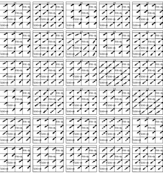
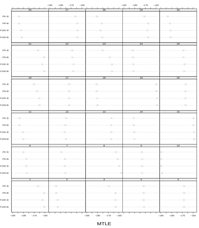
To present the simulation result, an LL plot is introduced, which is a sctterplot matrix of log-likelihood of several estimates. They include the forward search with or without a balance setting using a robust initial subset, denoted by “FR+B” and “FR-B”, and those using 100 random selected subsets, denoted by “F100+B” and “F100-B”. This plot is originally inspired by the RR plot of Hawkins and Olive (2002). The RR plot is a scatterplot matrix of the residuals from several regression fits. It is noted that the plot will be linear with slope 1 if the model assumptions hold.
Different configurations lead to quite similar results. Here we only show one of them to save the space. Figure 1 shows the LL plot of 30 simulated data set for n = 100 and k = 3. All scatterplots in each panel show linear relationship with slope 1. It concludes that all different setup lead to quite similar results in terms of likelihood values. It is noted that the pattern of the scatterplots of robust distances (??) from these approaches are similar to Figure 1. Therefore, they are not shown here.
Figure 2 shows the objective values (??) of 30 simulated dataset for the forward search algorithm using different options. All these values are quite close for each datasets. Figure 3 present the estimated cell probabilities of 30 simulated datasets for the forward search algorithm using different options. The empty cell may occur if the balance setting is not applied, which can be referred to the outlying cell. This also correspond to those different objective values in the panels in Figure 2.
===Figure 1 is here=== ===Figure 2 is here=== ===Figure 3 is here===
A robust start can lead to quite stable result as 100 random selected subset. However, the former one only spends almost 1/100 computation time than the latter one. Therefore, the forward search algorithm with a robust start is recommended. The balance setup remains an
important option for the approach because we never know whether outlying cells exit in data. If there is no outlying cell, the results with and without a balance setting lead to almost the same conclusion. If different conclusions are drawn, one should be careful to re-examine the data structure and an expert about the data may be called for further discussion.
3.4.2 The performance of the proposed approach
As the forward search algorithm for MTLE with a robust start performs no difference from that with 100 random search, we only use the former one in the following simulation study. The sample sizes 100 and 200 and dimensions p = 3, 5 and k = 2, 3 are generated. Each dataset contains 5, 10, 15, or 20 percent of bad data. For categorical data, each variable is generated from a binomial distribution with a success rate of 1/2. This actually results in that those cells follow a multinominal distribution with equal probability. Therefore, the balance setting is applied in the simulation study.
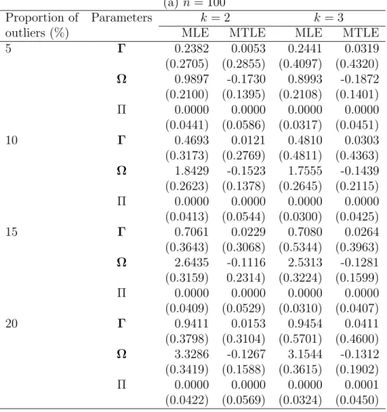
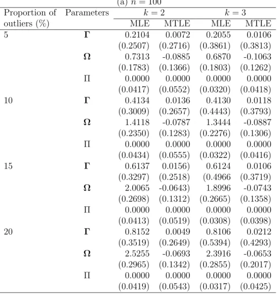
Tables 1 and 2 present the average bias of the estimates from 200 simulated data for
p = 3 and 5, respectively. The values in the parentheses denote the average MSE of the
estimates. These simulation results show that the performance of MTLE is more stable than MLE when different proportions of outliers are included in the data. The bias becomes larger for MLE when the proportion outliers turn large. It is noted that there is no difference of the estimate of Π between both estimates, because the cell probability is set to be equal in the simulated data.
In order to save computational time, the values of s are 2 and 4 for the sample sizes 100 and 200, respectively, when applying the forward search algorithm for MTLE. Of course, in some cases, we may obtain better results for the same dimension and the same sample size if we let s = 1 or some other small values. The default value of q is set to be [0.75n], which is also used in the real data analysis. For the dataset with 20% outliers, the value of q is [0.7n]. We can also expect that the greater the values are of q (provided that the value is not too large to include outliers), the better the simulation results will be.
===Table 1 is here=== ===Table 2 is here===
3.5
Outliers in mixed data
The simulations in the previous subsection assumed that outliers only occur in the continuous part of the data. However, in practice, we may have outliers only from the categorical part as well as outliers from both continuous and categorical parts of the data. If, in addition,
the categorical part is further contaminated (as in Bartlett and Lewis (1994) and Basu and Basu (1998)), then MTLE could work better. We do not compare MTLE with Bartlett and Lewis (1994) and Basu and Basu (1998), because the problem is different. The MTLE could be an alternative of Shane and Simonoff (2001). All these will be future studies.
The simulation study in subsection 3.4.1 has shown the proposed approach is able to identify outlier observations as well as outlying cells. A real data example is presented later to address this issue again. However, the simulation design excludes outliers from both con-tinuous and categorical variables in subsection 3.4.1. This is due to some remarks as follows. Firstly, the main concern here is ’observation’, where ’cell’ is the topic of Basu and Basu (1998) and Shane and Simonoff (2001)), in which there is no continuous variable. Therefore, an outlying cell will lead to all cases in that cell being outliers. On the other hand, if all observations in a cell are revealled as outliers, then this cell will be an outlying cell. Sec-ondly, according to the well-recognized definition of outliers in contingency table, an outlying cell (or frequency) is its frequency that deviates from the corresponding expected frequency about the null model (e.g. Barnett and Lewis (1994) and Basu and Basu (1998)). Therefore, a test of the cell probabilities can be carried out based upon the null model. However, we would never know the cell probability of the true null model in practice, especially when mixed data are present. Hence, in the process of the forward search algorithm, a balanced design is introduced to keep at least one observation in each cell as we mentioned before. Finally, it will be more difficult to identify an outlier from the continuous part than that from the discrete part (e.g. the discussion of the regression problem in Maronna and Yohai (2000)). Nevertheless, this paper focus on the identification of outlying observations, while outlying cells can therefore be revealled.
4
Examples
In this section, two real data examples are used to illustrate the MTLE method for mixed continuous and categorical data.
4.1
Nambeware polishing times data
The relation between polishing time and product diameters as well as type of product (casse-role, other) is one which is useful to a company for estimating the polishing time for new products which are designed or suggested for design and manufacture. This dataset can be downloaded from http://lib.stat.cmu.edu/DASL/Datafiles/nambedat.html. There are 59
cases and 4 dummy variables and 3 continuous variables in this dataset, which are described as below:
BOWL: Bowl (1) or not (0) CASS: Casserole (1) or not (0) DISH: Dish (1) or not (0) TRAY: Tray (1) or not (0)
DIAM: Diameter of item, or equivalent (inches) TIME: Grinding and polishing time (minutes) PRICE: Retail price ($)
The 4 dummy variables form 5 categories and the MLE estimates of parameters are listed in Table 3.
===Table 3 is here===
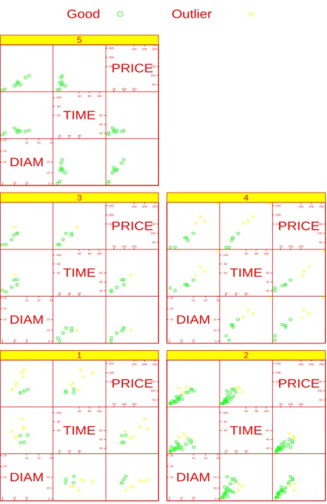
Applying the forward search algorithm for MTLE to these data, Table 4 gives the esti-mates of θ, which are quite different from those in Table 3. The corresponding Mahalanobis distances based on MLE and MTLE are shown in plots (a) and (b) of Figure 4, respectively. None of the cases appears to be outlying as shown in plot (a), while there are 14 outliers revealled when robust estimates are used. To check out the difference, Figure 5 shows the scatter matrix of those continuous variables by cell. Outliers belong to categories 1 and 4. This results in the different estimates of Tables 3 and 4.
It is noted that no matter what options, such as balance setting and starting subset, are used in the forward search algorithm, the same results are obtained for this data example.
===Table 4 is here=== ===Figure 4 is here=== ===Figure 5 is here===
4.2
Appendicitis data
The second dataset comes from Fisher and van Bell (1993, pp. 680-3) as an example of discriminant analysis, and it is originally from Koepsel et al. (1981). The data show the occurrence and non-occurrence of the perforation of the appendix. De Leon and Carri`ere (2005) also used this dataset to show their generalized Mahalanobis distances for mixed
data. There are 192 patients and 7 variables listed in Fisher and van Bell (1993), in which 4 continuous variables are described as below:
X2: age in years
X3: duration of symptoms in hours prior to physician contact
X4: time from physician contact to operation (in hours)
X5: white blood count in thousands
The other 3 dummy variables form 7 categories as presented in Table 5. It is noted that
we take logarithms on X2, X3, and X4. Missing values are excluded from the analysis, which
result in 179 cases in the following analysis. The case number appearing in the latter plot is the same as that shown in Fisher and van Bell (1993).
===Table 5 is here===
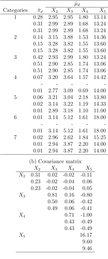
Applying the MLE and MTLE with and without a balance setting in the forward search for these data, Table 6 shows the results of the different estimates. The first line of each panel in Table 6 is the MLE, the second one is the MTLE without a balance setting in the forward search, and the last one is the MTLE with a balance setting in the forward search. As discussed in subsection 3.5, we can see that complicated and different situations may happen in the detection of outliers for the mixture data. The important feature of this difference is due to the outlying cells in the analysis. There is only one observation in category 6 and 4 cases to category 7.
If the balance design is not applied, then the cell probabilities of categories 4 and 6 are zero. The whole observations in these two categories are then excluded from the data in the forward procedure. This leads to zero cell mean estimates for these two categories. However, if the balance setting is considered in the forward process, then the observation of category 6 will have a guarantee to keep in the robust fit. Another interesting feature in Table 6 is that no matter whether the balance setting is applied or not, there is no difference in the MTL estimates of cell probabilities and cell means for categories 1, 2, and 3. The MTLEs of
the covariance matrix corresponding to variables X2, X3, and X4 are also the same for the
situations when the balance design is used and not used. Nevertheless, the results of MTLE are quite different from those of MLE.
===Table 6 is here===
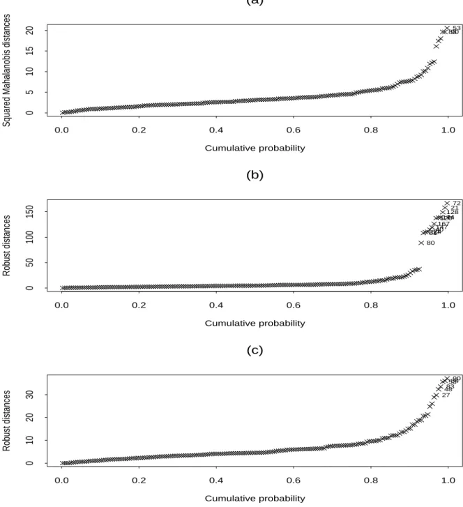
To see the effect of the different estimates on the identification of outliers, we can look at the Mahalanobis distances and the scatter plots. The corresponding Mahalanobis distances
based on MLE and MTLE without and with balance setting are shown in plots (a), (b), and (c) of Figure 6, respectively. Because of zero cell means occur in MTLE without the balance setting, this yields relatively large values of the distances than the other two methods. Both Figures 7 and 8 show the scatter matrix of those continuous variables by cell, but those outliers revealed by the former are applying the forward search algorithm with a balance setting, and the latter figure ignores the balance setting for the cell probability. It is clear to see that outliers appear to be away from the bulk of observations in each panel (cell) in both figures, except that the entire cases of categories 4 and 6 are revealed as outliers when the balance design is not used in Figure 8. It is noted that the case in cell 6 is located in the majority of data if only continuous variables are considered.
To examine the effect of the balanced setting, the corresponding optimum of (??) for MTLE without a balanced setting is −358.5531, and it is −360.1665 with a balanced setting. Therefore, in this case we may conclude that those values of the second line in Table 6 will be the better MTL estimates for these data.
===Figure 6 is here=== ===Figure 7 is here=== ===Figure 8 is here===
5
Conclusions
In this paper we propose the maximum trimmed likelihood estimates for multivariate data mixed with continuous and categorical variables. Given an initial small subset, intended to be outlier-free, the forward search algorithm can be relatively fast to compute the proposed MTL estimates. A simulation study shows that MTLE outperforms the classical MLE when an appropriate proportion of outliers exist in data. Real data are used to illustrate the proposed method. The results of the detection of outliers by MTLE are significantly different from those by MLE. One of the real data examples shows that the outliers from the categorical part may remain further examined, which will rely on the decision of the users. Nevertheless, the proposed method is able to deal with the robust diagnostic problem of outliers for mixture data.
There still exist some broader issues related to the mixture data and the method dis-cussed in the present paper. From the theoretical part, the statistical and robust properties of MTLE, such as breakdown point and efficiency, are needed to be verified. For the ap-plication of multivariate data, the MTLE can be extended to factor analysis, discriminant analysis and cluster analysis for mixture data. A decisive conclusion may be very important
to analysts for the identification of outliers from the categorical part.
References
Atkinson, A. C. (1994) “Fast Very Robust Methods for the Detection of Multiple Outliers,”
Journal of the American Statistical Association, 89, 1329-1339.
Atkinson, A. C. and Riani, M. (2000) Robust Diagnostic and Regression Analysis, New York: Springer-Verlag.
Atkinson, A. C., Riani, M. and Cerioli, A. (2004) Exploring Multivariate Data with the
Forward Search, New York: Springer.
Bar-Hen, A. and Daudin, J. J. (1995) “Generalization of the Mahalanobis Distance in the Mixed Case,” Journal of Multivariate Analysis, 53, 332-342.
Barnett,V. and Lewis, T. (1994) Outliers in Statistical Data, 3rd ed., New York: Wiley. Basu, A. and Basu, S. (1998) “Penalized Minimum Disparity Methods for Multinomial
Models,” Statistica Sinica, 841-860.
Bedrick, E. J., Lapidus, J. and Powell, J. F. (2000) “Estimating the Mahalanobis Distance from Mixed Continuous and Discrete Data,” Biometrics, 56, 394-401.
Butler, R. W., Davies, P. L. and Jhun, M. (1993) “Asymptotics for the Minimum Covariance Determinant Estimator,” The Annals of Statistics, 21, 1385-1400.
Cheng, T.-C. (2005) “Robust Regression Diagnostics With Data Transformations,”
Com-putational Statistics and Data Analysis, 49, 875-891.
Cheng, T.-C. and Victoria-Feser, M.-P. (2002) “High Breakdown Estimation of Multivariate Location and Scale With Missing Observations,” British Journal of Mathematical and
Statistical Psychology, 55, 317-335.
Croux, C. and Haesbroeck, G. (1999) “Influence function and efficiency of the minimum covariance determinant scatter matrix estimator,” Journal of Multivariate Analysis, 71, 161-190.
de Leon, A. R. and Carri´ere, K. C. (2005) “A Generalized Mahalanobis Distance for Mixed Data,” Journal of Multivariate Analysis, 92, 174-185.
Fisher, L. D. and van Bell, G. (1993) Biostatistics: A Methodology for the Health Science, New York: Wiley.
Hadi, A. S. and Luce˜no, A. (1997) “Maximum Trimmed Likelihood Estimators: a Unified Approach, Examples, and Algorithms,” Computational Statistics & Data Analysis, 25, 251-272.
Hawkins, D. M. (1994) “The Feasible Solution Algorithm for the Minimum Covariance De-terminant Estimator in Multivariate Data,” Computational Statistics & Data Analysis, 17, 197-210.
Hawkins, D. M. and Olive, D. J. (2002) “Inconsistency of resampling algorithms for high-breakdown regression estimators and a new algorithm” (with discussion), Journal of
the American Statistical Association, 97, 136-159.
Hubert, M. and Rousseeuw, P. J. (1997) “Robust Regression With Both Continuous and Binary Regressors,” Journal of Statistical Planning and Inference, 57, 153-163. Koepsel, T. D., Inui, T. S., and Farewell, V. T. (1981) “Factors Affecting Perforation in
Acute Appendicitis,” Surgery, Gynecology and Obstetrics, 153, 508-510.
Krzanowski, W. J. (1983) “Distance Between Populations using Mixed Continuous and. Categorical Variables,” Biometrika, 70, 235-243.
Little, R. J. A. and Rubin, D. B. (1987), Statistical Analysis with Missing Data, New York: John Wiley.
Maronna, R. A. and Yohai, V. J. (2000) “Robust Regression With Both Continuous and Categorical Predictors,” Journal of Statistical Planning and Inference, 89, 197-214. M¨uller, C. H., Neykov, N. (2003) “Breakdown Points of Trimmed Likelihood Estimators
and Related Estimators in Generalized Linear Models,” Journal of Statistical Planning
and Inference, 116, 503-519.
Olkin, I. and Tate, R. F. (1961) “Multivariate Correlation Models with Mixed Discrete and Continuous Variables,” Annals of Mathematical Statistics, 32, 448-465.
Rocke, D. M. and Woodruff, D. L. (1996) “Identification of Outliers in Multivariate Data,”
Rocke, D. M. and Woodruff, D. L. (1997) “Robust Estimation of Multivariate Location and Shape,” Journal of Statistical Planning and Inference, 57, 245-255.
Rousseeuw, P. J. and Leroy, A. M. (1987) Robust Regression and Outlier Detection, New York: John Wiley.
Rousseeuw, P. J. and van Driessen, K. (1999) “A Fast Algorithm for the Minimum Covari-ance Determinant Estimator,” Technometrics, 41, 212-223.
Rousseeuw, P. J. and van Zomeren, B. C. (1990) “Unmasking Multivariate Outliers and Leverage Points” (with discussion), Journal of the American Statistical Association, 85, 633-651.
Schafer, J. L. (1997), Analysis of Incomplete Multivariate Data, London: Chapman & Hall. Shane, K. V. and Simonoff, J. S. (2001) “A Robust Approach to Categorical Data Analysis,”
Journal of Computational and Graphical Statistics, 10, 135-157.
Woodruff and Rocke (1994) “Computable Robust Estimation of Multivariate Location and Shape in High Dimension Using Compound Estimators”, Journal of the American
Statistical Association, 89, 888-896.
Zaman, A., Rousseeuw, P. J., Orhan, M. (2001) “Econometric Applications of High-Breakdown Robust Regression Techniques,” Econometrics Letters, 71, 1-8.
Table 1. The simulation results (for bias) for p = 3. (a) n = 100
Proportion of Parameters k = 2 k = 3
outliers (%) MLE MTLE MLE MTLE
5 Γ 0.2382 0.0053 0.2441 0.0319 (0.2705) (0.2855) (0.4097) (0.4320) Ω 0.9897 -0.1730 0.8993 -0.1872 (0.2100) (0.1395) (0.2108) (0.1401) Π 0.0000 0.0000 0.0000 0.0000 (0.0441) (0.0586) (0.0317) (0.0451) 10 Γ 0.4693 0.0121 0.4810 0.0303 (0.3173) (0.2769) (0.4811) (0.4363) Ω 1.8429 -0.1523 1.7555 -0.1439 (0.2623) (0.1378) (0.2645) (0.2115) Π 0.0000 0.0000 0.0000 0.0000 (0.0413) (0.0544) (0.0300) (0.0425) 15 Γ 0.7061 0.0229 0.7080 0.0264 (0.3643) (0.3068) (0.5344) (0.3963) Ω 2.6435 -0.1116 2.5313 -0.1281 (0.3159) 0.2314) (0.3224) (0.1599) Π 0.0000 0.0000 0.0000 0.0000 (0.0409) (0.0529) (0.0310) (0.0407) 20 Γ 0.9411 0.0153 0.9454 0.0411 (0.3798) (0.3104) (0.5701) (0.4600) Ω 3.3286 -0.1267 3.1544 -0.1312 (0.3419) (0.1588) (0.3615) (0.1902) Π 0.0000 0.0000 0.0000 0.0001 (0.0422) (0.0569) (0.0324) (0.0450)
(b) n = 200
Proportion of Parameters k = 2 k = 3
outliers (%) MLE MTLE MLE MTLE
5 Γ 0.2412 0.0038 0.2354 0.0111 (0.1964) (0.2069) (0.2857) (0.3285) Ω 1.0097 -0.1740 0.9764 -0.1722 (0.1515) (0.1009) (0.1495) (0.1047) Π 0.0000 0.0000 0.0000 0.0000 (0.0302) (0.0415) (0.0232) (0.0333) 10 Γ 0.4709 0.0024 0.4701 0.0125 (0.2178) (0.1907) (0.3353) (0.3082) Ω 1.8930 -0.1454 1.8629 -0.1391 (0.1899 (0.1040) (0.1946) (0.1252) Π 0.0000 0.0000 0.0000 0.0000 0.0292 (0.0390) (0.0235) (0.0318) 15 Γ 0.7035 0.0034 0.7038 0.0173 (0.2470 (0.1898) (0.3752) (0.2895) Ω 2.7082 -0.1188 2.6461 -0.0973 (0.2232 (0.1003) (0.2206) (0.2390) Π 0.0000 0.0000 0.0000 0.0000 (0.0291 (0.0373) (0.0227) (0.0295) 20 Γ 0.9343 0.0045 0.9293 0.0087 (0.2699 (0.2055) (0.3941) (0.2755) Ω 3.3903 -0.1217 3.3177 -0.1190 (0.2516 (0.1850) (0.2440) (0.1266) Π 0.0000 0.0000 0.0000 0.0000 (0.0300 (0.0393) (0.0235) (0.0327)
Table 2. The simulation results (for bias) for p = 5. (a) n = 100
Proportion of Parameters k = 2 k = 3
outliers (%) MLE MTLE MLE MTLE
5 Γ 0.2104 0.0072 0.2055 0.0106 (0.2507) (0.2716) (0.3861) (0.3813) Ω 0.7313 -0.0885 0.6870 -0.1063 (0.1783) (0.1366) (0.1803) (0.1262) Π 0.0000 0.0000 0.0000 0.0000 (0.0417) (0.0552) (0.0320) (0.0418) 10 Γ 0.4134 0.0136 0.4130 0.0118 (0.3009) (0.2657) (0.4443) (0.3793) Ω 1.4118 -0.0787 1.3444 -0.0887 (0.2350) (0.1283) (0.2276) (0.1306) Π 0.0000 0.0000 0.0000 0.0000 (0.0434) (0.0555) (0.0322) (0.0416) 15 Γ 0.6137 0.0156) 0.6124 0.0106 (0.3297) (0.2518) (0.4966 (0.3719) Ω 2.0065 -0.0643) 1.8996 -0.0743 (0.2698) (0.1312) (0.2665) (0.1358) Π 0.0000 0.0000 0.0000 0.0000 (0.0413) (0.0519) (0.0308) (0.0398) 20 Γ 0.8152 0.0049 0.8106 0.0212 (0.3519) (0.2649) (0.5394) (0.4293) Ω 2.5255 -0.0693 2.3916 -0.0653 (0.2965) (0.1342) (0.2855) (0.2017) Π 0.0000 0.0000 0.0000 0.0000 (0.0419) (0.0543) (0.0317) (0.0425)
(b) n = 200
Proportion of Parameters k = 2 k = 3
outliers (%) MLE MTLE MLE MTLE
5 Γ 0.2064 0.0069 0.2065 0.0039 (0.1787) (0.1860) (0.2681) (0.2774) Ω 0.7576 -0.0883 0.7359 -0.0945 (0.1297) (0.0960) (0.1306) (0.0939) Π 0.0000 0.0000 0.0000 0.0000 (0.0303) (0.0395) (0.0226) (0.0310) 10 Γ 0.4100 0.0064 0.4079 0.0013 (0.2141) (0.1860) (0.3077) (0.2670) Ω 1.4461 -0.0768 1.4045 -0.0799 (0.1628) (0.0964) (0.1587) (0.0979) Π 0.0000 0.0000 0.0000 0.0000 (0.0296) (0.0380) (0.0225) (0.0295) 15 Γ 0.6116 0.0030 0.6098 0.0064 (0.2335) (0.1794) (0.3340) (0.2592) Ω 2.0581 -0.0598 2.0061 -0.0657 (0.1870) (0.0957) (0.1878) (0.0954) Π 0.0000 0.0000 0.0000 0.0000 (0.0311) (0.0381) (0.0231) (0.0290) 20 Γ 0.8130 0.0022 0.8127 0.0052 (0.2509) (0.1914) (0.3693) (0.2736) Ω 2.5737 -0.0676 2.5189 -0.0744 (0.2074) (0.0986) (0.2091) (0.0965) Π 0.0000 0.0000 0.0000 0.0000 (0.0322) (0.0407) (0.0224) (0.0299)
Table 3. MLE for Nambeware polishing times data. (a) Expected frequencies and cell means
Cell µˆd
Categories BOWL CASS DISH TRAY πˆd DIAM TIME PRICE
1 0 1 0 0 0.17 12.49 53.26 135.75 2 1 0 0 0 0.39 9.44 27.12 67.39 3 0 0 1 0 0.12 8.89 35.01 80.14 4 0 0 0 1 0.17 14.28 49.40 112.15 5 0 0 0 0 0.15 10.86 24.19 56.28 (b) Covariance matrix
DIAM TIME PRICE
DIAM 10.91 32.73 114.57
TIME 222.52 562.48
PRICE 1805.44
Table 4. MTLE for Nambeware polishing times data. (a) Expected frequencies and cell means
Cell µˆd
Categories BOWL CASS DISH TRAY πˆd DIAM TIME PRICE
1 0 1 0 0 0.09 13.55 41.20 96.62 2 1 0 0 0 0.44 9.26 24.00 61.10 3 0 0 1 0 0.13 8.70 31.59 71.17 4 0 0 0 1 0.13 10.75 31.83 58.75 5 0 0 0 0 0.20 10.86 24.19 56.28 (b) Covariance matrix DIAM TIME PRICE
DIAM 8.29 13.66 67.60
TIME 57.53 139.33
PRICE 619.32
Table 5. Cells for appendicitis data.
Perforation status Sex Gangrene Frequency
Category (1=yes; 0=no) (1=male; 0=female) (1=yes; 0=no)
1 0 0 0 51 2 1 1 1 25 3 0 1 0 76 4 1 0 1 12 5 0 1 1 10 6 1 0 0 1 7 0 0 1 4
Table 6. MTLE for appendicitis data. (a) Expected frequencies and cell means
ˆ µd Categories πˆd X2 X3 X4 X5 1 0.28 2.95 2.95 1.80 13.14 0.31 2.99 2.89 1.68 13.24 0.31 2.99 2.89 1.68 13.24 2 0.14 3.15 3.88 1.53 14.36 0.15 3.28 3.82 1.55 13.60 0.15 3.28 3.82 1.55 13.60 3 0.42 2.93 2.99 1.80 13.24 0.51 2.90 2.85 1.74 13.06 0.51 2.90 2.85 1.74 13.06 4 0.07 3.20 3.64 1.57 14.42 - - - - -0.01 2.77 3.09 0.69 14.00 5 0.06 3.21 3.04 2.18 13.80 0.02 3.14 3.22 1.19 14.33 0.01 2.89 3.18 1.10 11.00 6 0.01 3.14 5.12 1.61 18.00 - - - - -0.01 3.14 5.12 1.61 18.00 7 0.02 2.96 2.62 1.84 15.25 0.01 2.94 3.87 2.20 14.00 0.01 2.94 3.87 2.20 14.00 (b) Covariance matrix X2 X3 X4 X5 X2 0.31 0.02 -0.02 -0.11 0.23 -0.02 -0.04 0.06 0.23 -0.02 -0.04 0.05 X3 0.81 0.16 -0.80 0.50 0.06 -0.42 0.49 0.06 -0.41 X4 0.71 -1.00 0.43 -0.49 0.43 -0.49 X5 16.17 9.60 9.46
1 −140−120−100 −80 −80 −60 −40 −20 −80 −60 −40 −20 −140 −120 −100 −80 F100+B −140−120−100 −80 −80 −60 −40 −20 −80 −60 −40 −20 −140 −120 −100 −80 F100−B −140−120−100 −80 −80 −60 −40 −20 −80 −60 −40 −20 −140 −120 −100 −80 FR+B −140−120−100 −80 −80 −60 −40 −20 −80 −60 −40 −20 −140 −120 −100 −80 FR−B 2 −140−120−100 −80 −80 −60 −40 −20 −80 −60 −40 −20 −140 −120 −100 −80 F100+B −140−120−100 −80 −80 −60 −40 −20 −80 −60 −40 −20 −140 −120 −100 −80 F100−B −140−120−100 −80 −80 −60 −40 −20 −80 −60 −40 −20 −140 −120 −100 −80 FR+B −140−120−100 −80 −80 −60 −40 −20 −80 −60 −40 −20 −140 −120 −100 −80 FR−B 3 −140−120−100 −80 −80 −60 −40 −20 −80 −60 −40 −20 −140 −120 −100 −80 F100+B −140−120−100 −80 −80 −60 −40 −20 −80 −60 −40 −20 −140 −120 −100 −80 F100−B −140−120−100 −80 −80 −60 −40 −20 −80 −60 −40 −20 −140 −120 −100 −80 FR+B −140−120−100 −80 −80 −60 −40 −20 −80 −60 −40 −20 −140 −120 −100 −80 FR−B 4 −140−120−100 −80 −80 −60 −40 −20 −80 −60 −40 −20 −140 −120 −100 −80 F100+B −140−120−100 −80 −80 −60 −40 −20 −80 −60 −40 −20 −140 −120 −100 −80 F100−B −140−120−100 −80 −80 −60 −40 −20 −80 −60 −40 −20 −140 −120 −100 −80 FR+B −140−120−100 −80 −80 −60 −40 −20 −80 −60 −40 −20 −140 −120 −100 −80 FR−B 5 −140−120−100 −80 −80 −60 −40 −20 −80 −60 −40 −20 −140 −120 −100 −80 F100+B −140−120−100 −80 −80 −60 −40 −20 −80 −60 −40 −20 −140 −120 −100 −80 F100−B −140−120−100 −80 −80 −60 −40 −20 −80 −60 −40 −20 −140 −120 −100 −80 FR+B −140−120−100 −80 −80 −60 −40 −20 −80 −60 −40 −20 −140 −120 −100 −80 FR−B 6 −140−120−100 −80 −80 −60 −40 −20 −80 −60 −40 −20 −140 −120 −100 −80 F100+B −140−120−100 −80 −80 −60 −40 −20 −80 −60 −40 −20 −140 −120 −100 −80 F100−B −140−120−100 −80 −80 −60 −40 −20 −80 −60 −40 −20 −140 −120 −100 −80 FR+B −140−120−100 −80 −80 −60 −40 −20 −80 −60 −40 −20 −140 −120 −100 −80 FR−B 7 −140−120−100 −80 −80 −60 −40 −20 −80 −60 −40 −20 −140 −120 −100 −80 F100+B −140−120−100 −80 −80 −60 −40 −20 −80 −60 −40 −20 −140 −120 −100 −80 F100−B −140−120−100 −80 −80 −60 −40 −20 −80 −60 −40 −20 −140 −120 −100 −80 FR+B −140−120−100 −80 −80 −60 −40 −20 −80 −60 −40 −20 −140 −120 −100 −80 FR−B 8 −140−120−100 −80 −80 −60 −40 −20 −80 −60 −40 −20 −140 −120 −100 −80 F100+B −140−120−100 −80 −80 −60 −40 −20 −80 −60 −40 −20 −140 −120 −100 −80 F100−B −140−120−100 −80 −80 −60 −40 −20 −80 −60 −40 −20 −140 −120 −100 −80 FR+B −140−120−100 −80 −80 −60 −40 −20 −80 −60 −40 −20 −140 −120 −100 −80 FR−B 9 −140−120−100 −80 −80 −60 −40 −20 −80 −60 −40 −20 −140 −120 −100 −80 F100+B −140−120−100 −80 −80 −60 −40 −20 −80 −60 −40 −20 −140 −120 −100 −80 F100−B −140−120−100 −80 −80 −60 −40 −20 −80 −60 −40 −20 −140 −120 −100 −80 FR+B −140−120−100 −80 −80 −60 −40 −20 −80 −60 −40 −20 −140 −120 −100 −80 FR−B 10 −140−120−100 −80 −80 −60 −40 −20 −80 −60 −40 −20 −140 −120 −100 −80 F100+B −140−120−100 −80 −80 −60 −40 −20 −80 −60 −40 −20 −140 −120 −100 −80 F100−B −140−120−100 −80 −80 −60 −40 −20 −80 −60 −40 −20 −140 −120 −100 −80 FR+B −140−120−100 −80 −80 −60 −40 −20 −80 −60 −40 −20 −140 −120 −100 −80 FR−B 11 −140−120−100 −80 −80 −60 −40 −20 −80 −60 −40 −20 −140 −120 −100 −80 F100+B −140−120−100 −80 −80 −60 −40 −20 −80 −60 −40 −20 −140 −120 −100 −80 F100−B −140−120−100 −80 −80 −60 −40 −20 −80 −60 −40 −20 −140 −120 −100 −80 FR+B −140−120−100 −80 −80 −60 −40 −20 −80 −60 −40 −20 −140 −120 −100 −80 FR−B 12 −140−120−100 −80 −80 −60 −40 −20 −80 −60 −40 −20 −140 −120 −100 −80 F100+B −140−120−100 −80 −80 −60 −40 −20 −80 −60 −40 −20 −140 −120 −100 −80 F100−B −140−120−100 −80 −80 −60 −40 −20 −80 −60 −40 −20 −140 −120 −100 −80 FR+B −140−120−100 −80 −80 −60 −40 −20 −80 −60 −40 −20 −140 −120 −100 −80 FR−B 13 −140−120−100 −80 −80 −60 −40 −20 −80 −60 −40 −20 −140 −120 −100 −80 F100+B −140−120−100 −80 −80 −60 −40 −20 −80 −60 −40 −20 −140 −120 −100 −80 F100−B −140−120−100 −80 −80 −60 −40 −20 −80 −60 −40 −20 −140 −120 −100 −80 FR+B −140−120−100 −80 −80 −60 −40 −20 −80 −60 −40 −20 −140 −120 −100 −80 FR−B 14 −140−120−100 −80 −80 −60 −40 −20 −80 −60 −40 −20 −140 −120 −100 −80 F100+B −140−120−100 −80 −80 −60 −40 −20 −80 −60 −40 −20 −140 −120 −100 −80 F100−B −140−120−100 −80 −80 −60 −40 −20 −80 −60 −40 −20 −140 −120 −100 −80 FR+B −140−120−100 −80 −80 −60 −40 −20 −80 −60 −40 −20 −140 −120 −100 −80 FR−B 15 −140−120−100 −80 −80 −60 −40 −20 −80 −60 −40 −20 −140 −120 −100 −80 F100+B −140−120−100 −80 −80 −60 −40 −20 −80 −60 −40 −20 −140 −120 −100 −80 F100−B −140−120−100 −80 −80 −60 −40 −20 −80 −60 −40 −20 −140 −120 −100 −80 FR+B −140−120−100 −80 −80 −60 −40 −20 −80 −60 −40 −20 −140 −120 −100 −80 FR−B 16 −140−120−100 −80 −80 −60 −40 −20 −80 −60 −40 −20 −140 −120 −100 −80 F100+B −140−120−100 −80 −80 −60 −40 −20 −80 −60 −40 −20 −140 −120 −100 −80 F100−B −140−120−100 −80 −80 −60 −40 −20 −80 −60 −40 −20 −140 −120 −100 −80 FR+B −140−120−100 −80 −80 −60 −40 −20 −80 −60 −40 −20 −140 −120 −100 −80 FR−B 17 −140−120−100 −80 −80 −60 −40 −20 −80 −60 −40 −20 −140 −120 −100 −80 F100+B −140−120−100 −80 −80 −60 −40 −20 −80 −60 −40 −20 −140 −120 −100 −80 F100−B −140−120−100 −80 −80 −60 −40 −20 −80 −60 −40 −20 −140 −120 −100 −80 FR+B −140−120−100 −80 −80 −60 −40 −20 −80 −60 −40 −20 −140 −120 −100 −80 FR−B 18 −140−120−100 −80 −80 −60 −40 −20 −80 −60 −40 −20 −140 −120 −100 −80 F100+B −140−120−100 −80 −80 −60 −40 −20 −80 −60 −40 −20 −140 −120 −100 −80 F100−B −140−120−100 −80 −80 −60 −40 −20 −80 −60 −40 −20 −140 −120 −100 −80 FR+B −140−120−100 −80 −80 −60 −40 −20 −80 −60 −40 −20 −140 −120 −100 −80 FR−B 19 −140−120−100 −80 −80 −60 −40 −20 −80 −60 −40 −20 −140 −120 −100 −80 F100+B −140−120−100 −80 −80 −60 −40 −20 −80 −60 −40 −20 −140 −120 −100 −80 F100−B −140−120−100 −80 −80 −60 −40 −20 −80 −60 −40 −20 −140 −120 −100 −80 FR+B −140−120−100 −80 −80 −60 −40 −20 −80 −60 −40 −20 −140 −120 −100 −80 FR−B 20 −140−120−100 −80 −80 −60 −40 −20 −80 −60 −40 −20 −140 −120 −100 −80 F100+B −140−120−100 −80 −80 −60 −40 −20 −80 −60 −40 −20 −140 −120 −100 −80 F100−B −140−120−100 −80 −80 −60 −40 −20 −80 −60 −40 −20 −140 −120 −100 −80 FR+B −140−120−100 −80 −80 −60 −40 −20 −80 −60 −40 −20 −140 −120 −100 −80 FR−B 21 −140−120−100 −80 −80 −60 −40 −20 −80 −60 −40 −20 −140 −120 −100 −80 F100+B −140−120−100 −80 −80 −60 −40 −20 −80 −60 −40 −20 −140 −120 −100 −80 F100−B −140−120−100 −80 −80 −60 −40 −20 −80 −60 −40 −20 −140 −120 −100 −80 FR+B −140−120−100 −80 −80 −60 −40 −20 −80 −60 −40 −20 −140 −120 −100 −80 FR−B 22 −140−120−100 −80 −80 −60 −40 −20 −80 −60 −40 −20 −140 −120 −100 −80 F100+B −140−120−100 −80 −80 −60 −40 −20 −80 −60 −40 −20 −140 −120 −100 −80 F100−B −140−120−100 −80 −80 −60 −40 −20 −80 −60 −40 −20 −140 −120 −100 −80 FR+B −140−120−100 −80 −80 −60 −40 −20 −80 −60 −40 −20 −140 −120 −100 −80 FR−B 23 −140−120−100 −80 −80 −60 −40 −20 −80 −60 −40 −20 −140 −120 −100 −80 F100+B −140−120−100 −80 −80 −60 −40 −20 −80 −60 −40 −20 −140 −120 −100 −80 F100−B −140−120−100 −80 −80 −60 −40 −20 −80 −60 −40 −20 −140 −120 −100 −80 FR+B −140−120−100 −80 −80 −60 −40 −20 −80 −60 −40 −20 −140 −120 −100 −80 FR−B 24 −140−120−100 −80 −80 −60 −40 −20 −80 −60 −40 −20 −140 −120 −100 −80 F100+B −140−120−100 −80 −80 −60 −40 −20 −80 −60 −40 −20 −140 −120 −100 −80 F100−B −140−120−100 −80 −80 −60 −40 −20 −80 −60 −40 −20 −140 −120 −100 −80 FR+B −140−120−100 −80 −80 −60 −40 −20 −80 −60 −40 −20 −140 −120 −100 −80 FR−B 25 −140−120−100 −80 −80 −60 −40 −20 −80 −60 −40 −20 −140 −120 −100 −80 F100+B −140−120−100 −80 −80 −60 −40 −20 −80 −60 −40 −20 −140 −120 −100 −80 F100−B −140−120−100 −80 −80 −60 −40 −20 −80 −60 −40 −20 −140 −120 −100 −80 FR+B −140−120−100 −80 −80 −60 −40 −20 −80 −60 −40 −20 −140 −120 −100 −80 FR−B 26 −140−120−100 −80 −80 −60 −40 −20 −80 −60 −40 −20 −140 −120 −100 −80 F100+B −140−120−100 −80 −80 −60 −40 −20 −80 −60 −40 −20 −140 −120 −100 −80 F100−B −140−120−100 −80 −80 −60 −40 −20 −80 −60 −40 −20 −140 −120 −100 −80 FR+B −140−120−100 −80 −80 −60 −40 −20 −80 −60 −40 −20 −140 −120 −100 −80 FR−B 27 −140−120−100 −80 −80 −60 −40 −20 −80 −60 −40 −20 −140 −120 −100 −80 F100+B −140−120−100 −80 −80 −60 −40 −20 −80 −60 −40 −20 −140 −120 −100 −80 F100−B −140−120−100 −80 −80 −60 −40 −20 −80 −60 −40 −20 −140 −120 −100 −80 FR+B −140−120−100 −80 −80 −60 −40 −20 −80 −60 −40 −20 −140 −120 −100 −80 FR−B 28 −140−120−100 −80 −80 −60 −40 −20 −80 −60 −40 −20 −140 −120 −100 −80 F100+B −140−120−100 −80 −80 −60 −40 −20 −80 −60 −40 −20 −140 −120 −100 −80 F100−B −140−120−100 −80 −80 −60 −40 −20 −80 −60 −40 −20 −140 −120 −100 −80 FR+B −140−120−100 −80 −80 −60 −40 −20 −80 −60 −40 −20 −140 −120 −100 −80 FR−B 29 −140−120−100 −80 −80 −60 −40 −20 −80 −60 −40 −20 −140 −120 −100 −80 F100+B −140−120−100 −80 −80 −60 −40 −20 −80 −60 −40 −20 −140 −120 −100 −80 F100−B −140−120−100 −80 −80 −60 −40 −20 −80 −60 −40 −20 −140 −120 −100 −80 FR+B −140−120−100 −80 −80 −60 −40 −20 −80 −60 −40 −20 −140 −120 −100 −80 FR−B 30 −140−120−100 −80 −80 −60 −40 −20 −80 −60 −40 −20 −140 −120 −100 −80 F100+B −140−120−100 −80 −80 −60 −40 −20 −80 −60 −40 −20 −140 −120 −100 −80 F100−B −140−120−100 −80 −80 −60 −40 −20 −80 −60 −40 −20 −140 −120 −100 −80 FR+B −140−120−100 −80 −80 −60 −40 −20 −80 −60 −40 −20 −140 −120 −100 −80 FR−B
F100+B F100−B FR+B FR−B −195 −185 −175 −165 1 2 −195 −185 −175 −165 3 4 −195 −185 −175 −165 5 F100+B F100−B FR+B FR−B 6 7 8 9 10 F100+B F100−B FR+B FR−B 11 12 13 14 15 F100+B F100−B FR+B FR−B 16 17 18 19 20 F100+B F100−B FR+B FR−B 21 22 23 24 25 F100+B F100−B FR+B FR−B 26 −195 −185 −175 −165 27 28 −195 −185 −175 −165 29 30 MTLE
Figure 2: The objective values of 30 simulated dataset for the forward search algorithm using different options.
F100+B F100−B FR+B FR−B MLE 0.0 0.10 0.20 1 2 0.0 0.10 0.20 3 4 0.0 0.10 0.20 5 F100+B F100−B FR+B FR−B MLE 6 7 8 9 10 F100+B F100−B FR+B FR−B MLE 11 12 13 14 15 F100+B F100−B FR+B FR−B MLE 16 17 18 19 20 F100+B F100−B FR+B FR−B MLE 21 22 23 24 25 F100+B F100−B FR+B FR−B MLE 26 0.0 0.10 0.20 27 28 0.0 0.10 0.20 29 30 Pi Cell 1 Cell 2 Cell 3 Cell 4 Cell 5 Cell 6 Cell 7 Cell 8
Figure 3: The estimated cell probabilities of 30 simulated dataset for the forward search algorithm using different options.
Cumulative probability
Squared Mahalanobis distances
0.0 0.2 0.4 0.6 0.8 1.0 0 5 10 15 (a) 11 2 37 Cumulative probability Robust distances 0.0 0.2 0.4 0.6 0.8 1.0 0 50 100 150 200 2 37 11 33 1 45 6 7 19 5 3 41 44 28 (b)
Figure 4: Nambeware polishing times data: (a) squared Mahalonobis distances based on MLE; (b) robust distances based on MTLE.
1 5 10 15 15 20 25 15 20 25 5 10 15 DIAM 20 40 60 60 80 100 60 80 100 20 40 60 TIME 50 100 150 150 200 250 150 200 250 50 100 150 PRICE 2 5 10 15 15 20 25 15 20 25 5 10 15 DIAM 20 40 60 60 80 100 60 80 100 20 40 60 TIME 50 100 150 150 200 250 150 200 250 50 100 150 PRICE 3 5 10 15 15 20 25 15 20 25 5 10 15 DIAM 20 40 60 60 80 100 60 80 100 20 40 60 TIME 50 100 150 150 200 250 150 200 250 50 100 150 PRICE 4 5 10 15 15 20 25 15 20 25 5 10 15 DIAM 20 40 60 60 80 100 60 80 100 20 40 60 TIME 50 100 150 150 200 250 150 200 250 50 100 150 PRICE 5 5 10 15 15 20 25 15 20 25 5 10 15 DIAM 20 40 60 60 80 100 60 80 100 20 40 60 TIME 50 100 150 150 200 250 150 200 250 50 100 150 PRICE Good Outlier
Cumulative probability
Squared Mahalanobis distances
0.0 0.2 0.4 0.6 0.8 1.0 0 5 10 15 20 (a) 53 90 83 Cumulative probability Robust distances 0.0 0.2 0.4 0.6 0.8 1.0 0 50 100 150 72 21 128 74 144 126 167 147 40 24 60 81 80 (b) Cumulative probability Robust distances 0.0 0.2 0.4 0.6 0.8 1.0 0 10 20 30 90 84 53 83 48 27 (c)
Figure 6: Appendicitis data: (a) squared Mahalonobis distances based on MLE; (b) robust distances based on MTLE without balance setting in the forward search; (c) robust distances based on MTLE with balance setting in the forward search.
1 1.52.02.5 3.03.54.0 3.0 3.5 4.0 1.5 2.0 2.5 X2 1 2 3 4 5 6 4 5 6 1 2 3 X3 0 1 2 3 4 5 3 4 5 0 1 2 X4 5 10 15 20 25 30 20 25 30 5 10 15 X5 2 1.52.02.5 3.03.54.0 3.0 3.5 4.0 1.5 2.0 2.5 X2 1 2 3 4 5 6 4 5 6 1 2 3 X3 0 1 2 3 4 5 3 4 5 0 1 2 X4 5 10 15 20 25 30 20 25 30 5 10 15 X5 3 1.52.02.5 3.03.54.0 3.0 3.5 4.0 1.5 2.0 2.5 X2 1 2 3 4 5 6 4 5 6 1 2 3 X3 0 1 2 3 4 5 3 4 5 0 1 2 X4 5 10 15 20 25 30 20 25 30 5 10 15 X5 4 1.52.02.5 3.03.54.0 3.0 3.5 4.0 1.5 2.0 2.5 X2 1 2 3 4 5 6 4 5 6 1 2 3 X3 0 1 2 3 4 5 3 4 5 0 1 2 X4 5 10 15 20 25 30 20 25 30 5 10 15 X5 5 1.52.02.5 3.03.54.0 3.0 3.5 4.0 1.5 2.0 2.5 X2 1 2 3 4 5 6 4 5 6 1 2 3 X3 0 1 2 3 4 5 3 4 5 0 1 2 X4 5 10 15 20 25 30 20 25 30 5 10 15 X5 6 1.52.02.5 3.03.54.0 3.0 3.5 4.0 1.5 2.0 2.5 X2 1 2 3 4 5 6 4 5 6 1 2 3 X3 0 1 2 3 4 5 3 4 5 0 1 2 X4 5 10 15 20 25 30 20 25 30 5 10 15 X5 7 1.52.02.5 3.03.54.0 3.0 3.5 4.0 1.5 2.0 2.5 X2 1 2 3 4 5 6 4 5 6 1 2 3 X3 0 1 2 3 4 5 3 4 5 0 1 2 X4 5 10 15 20 25 30 20 25 30 5 10 15 X5 Good Outlier
Figure 7: Appendicitis data: scatter matrix. Outliers are indicated by MTLE with balance setting in the forward search.
1 1.52.02.5 3.03.54.0 3.0 3.5 4.0 1.5 2.0 2.5 X2 1 2 3 4 5 6 4 5 6 1 2 3 X3 0 1 2 3 4 5 3 4 5 0 1 2 X4 5 10 15 20 25 30 20 25 30 5 10 15 X5 2 1.52.02.5 3.03.54.0 3.0 3.5 4.0 1.5 2.0 2.5 X2 1 2 3 4 5 6 4 5 6 1 2 3 X3 0 1 2 3 4 5 3 4 5 0 1 2 X4 5 10 15 20 25 30 20 25 30 5 10 15 X5 3 1.52.02.5 3.03.54.0 3.0 3.5 4.0 1.5 2.0 2.5 X2 1 2 3 4 5 6 4 5 6 1 2 3 X3 0 1 2 3 4 5 3 4 5 0 1 2 X4 5 10 15 20 25 30 20 25 30 5 10 15 X5 4 1.52.02.5 3.03.54.0 3.0 3.5 4.0 1.5 2.0 2.5 X2 1 2 3 4 5 6 4 5 6 1 2 3 X3 0 1 2 3 4 5 3 4 5 0 1 2 X4 5 10 15 20 25 30 20 25 30 5 10 15 X5 5 1.52.02.5 3.03.54.0 3.0 3.5 4.0 1.5 2.0 2.5 X2 1 2 3 4 5 6 4 5 6 1 2 3 X3 0 1 2 3 4 5 3 4 5 0 1 2 X4 5 10 15 20 25 30 20 25 30 5 10 15 X5 6 1.52.02.5 3.03.54.0 3.0 3.5 4.0 1.5 2.0 2.5 X2 1 2 3 4 5 6 4 5 6 1 2 3 X3 0 1 2 3 4 5 3 4 5 0 1 2 X4 5 10 15 20 25 30 20 25 30 5 10 15 X5 7 1.52.02.5 3.03.54.0 3.0 3.5 4.0 1.5 2.0 2.5 X2 1 2 3 4 5 6 4 5 6 1 2 3 X3 0 1 2 3 4 5 3 4 5 0 1 2 X4 5 10 15 20 25 30 20 25 30 5 10 15 X5 Good Outlier
Figure 8: Appendicitis data: scatter matrix. Outliers are indicated by MTLE without balance setting in the forward search.