國
立
交
通
大
學
資訊科學與工程研究所
碩
士
論
文
NFL 定理在離散化 Lipschitz 函數
集合上之探討
Free Lunch on the Discrete Lipschitz Class
研 究 生:江沛
指導教授:陳穎平 教授
NFL 定理在離散化 Lipschitz 函數集合上之探討
Free Lunch on the Discrete Lipschitz Class
研 究 生:江沛 Student:Pei Jiang
指導教授:陳穎平 Advisor:Ying-ping Chen
國 立 交 通 大 學
資 訊 科 學 與 工 程 研 究 所
碩 士 論 文
A ThesisSubmitted to Institute of Computer Science and Engineering College of Computer Science
National Chiao Tung University in partial Fulfillment of the Requirements
for the Degree of Master
in
Computer Science
June 2008
Hsinchu, Taiwan, Republic of China
NFL 定理在離散化 Lipschitz 函數集合上之探討
學生:江沛 指導教授:陳穎平
國立交通大學資訊科學與工程研究所
摘 要
No-Free-Lunch(NFL)定理指出當對所有問題作平均時,所有最佳化演算
法的表現都是一致的,意即各個最佳化演算法的總體效能並無法定義孰優孰
劣 。 然 而 NFL 定 理 並 不 意 味 著 泛 用 型 最 佳 化 演 算 法 (general-purpose
optimizers)無用武之地,只要問題存在有可供演算法利用的結構,仍有可能
找到一最佳化演算法在某一問題集合上具有優勢。這份論文提出了一個問題
的集合,稱之為離散化 Lipschitz 函數集合(discrete Lipschitz class,DLC),
且此一集合可視為透過規範搜尋空間鄰近區域的差值來模擬連續性。此論文
探 討 了 DLC 和 NFL 定 理 間 之 關 係 , 並 證 明 一 最 佳 化 演 算 法
subthreshold-seeker 之推廣形式可在 DLC 上效能勝於 random search。同時,
此 論 文 也 設 計 了 一 抽 樣 測 試 法 透 過 實 驗 驗 證 在 一 更 實 際 之 架 構 下
subthreshold-seeker 在 DLC 上之表現明顯優於 random search。因此,這份
論文說明了儘管最佳化演算法並無法同時對所有問題都有優異的效能,但仍
然有可能在一廣泛且深具意義的問題集合上取得優勢。
關鍵字:No-Free-Lunch 定理、Lipschitz 連續性、泛用型最佳化演算法、
subthreshold-seeker、抽樣測試法
Abstract
The No-Free-Lunch theorem states that all algorithms have the identical performance on average over all functions and there is no algorithm able to outperform others on all problems. However, such a result does not imply that search heuristics or optimization al-gorithms are futile if we are more cautious with the applicability of these methods and the search space. In this paper, within the No-Free-Lunch framework, we firstly introduce the discrete Lipschitz class by transferring the Lipschitz functions, i.e., functions with bounded slope, as a measure to fulfill the notion of continuity in discrete functions. We then in-vestigate the properties of the discrete Lipschitz class, generalize an algorithm called subthreshold-seeker for optimization, and show that the generalized subthreshold-seeker outperforms random search on this class. Finally, we propose a tractable sampling-test scheme to empirically demonstrate the superiority of the generalized subthreshold-seeker under practical configurations. This study concludes that there exists algorithms outper-forming random search on the discrete Lipschitz class in both theoretical and practical aspects and indicates that the effectiveness of search heuristics may not be universal but still general in some broad sense.
keywords:
No-Free-Lunch Theorem, Lipschitz continuity, discrete Lipschitz class, subthreshold-seeker, sampling-test scheme
誌
謝
現在時間是 2009 年七月七日下午三點十八分,我在自然計算實驗室
待了兩年的座位看著螢幕上一篇即將完結的論文,和即將完結的學生
歲月──從今以後再也不能買學生票了,想來還真有點感傷。因此,
以下將一一條列那些致使我接下來的人生得多付幾十塊錢才能看場
電影的重大功臣,聊表個人微不足道的巨大謝意:
1. 感謝父母的生育教養,那是一切的根源。
2. 感謝陳穎平老師的開明和適切指導,讓我能自在探索興趣,
一窺學術世界的堂奧。
3. 感謝口試委員:張時中老師、鄭士康老師、于天立老師的洞
見和寬容,讓我有機會精進這篇論文。
4. 感謝計算機中心校務資訊組提供我學習的機會,還有優渥的
工讀金,讓我不用為房租而煩惱。
5. 感謝三位室友一同度過兩年來的點點滴滴。
6. 感謝實驗室學長姐、同學、學弟妹的同舟共濟。
7. 感謝諸多親友的支持和陪伴。
8. 最後,我還要感謝亞利桑納響尾蛇在這兩年無緣季後賽,讓
我能心無旁騖的進行研究。
要感謝的人太多了,我很想繼續條列下去,但說明你們對我的幫助足
以寫成另一本論文。
Contents
Abstract iii
Table of Contents iv
List of Figures vi
List of Tables vii
1 Introduction 1 1.1 Motivation . . . 1 1.2 Research Objectives . . . 2 1.3 Road Map . . . 3 2 A Brief Review of NFL 4 2.1 NFL Framework . . . 4 2.2 NFL Theorem . . . 6
3 Discrete Lipschitz Class 7 3.1 Definition of the Discrete Lipschitz Class . . . 7
3.2 DLC as Representation . . . 8
3.2.1 Real-parameter Optimization Problems . . . 8
3.2.2 Combinatorial Optimization Problems . . . 9
3.3 DLC and NFL . . . 10
4 DLC and Subthreshold-seeker 13 4.1 Generalized Subthreshold-seeker . . . 13
5 Sampling-test Scheme for PDLC 21 5.1 A Uniform Sampler for PDLC . . . 21 5.2 Experimental Settings and Results . . . 25 5.3 The Estimation of Median . . . 29
6 Toward Higher Dimensions 31
6.1 Accept-reject Sampler for Planar DLC . . . 32 6.2 MCMC Sampler . . . 34 6.3 Semi-planar DLC . . . 36 7 Conclusions 40 7.1 Summary . . . 40 7.2 Main Conclusions . . . 40 7.3 Future Work . . . 41
List of Figures
2.1 An illustration of an algorithm . . . 5
3.1 A function instance of PDLC with 10 vertexes and K = 10. . . . 9
6.1 An instance of planar DLC with 202 vertexes and K = 10 . . . 31
6.2 an instance of planar DLC generated by Algorithm 3 . . . 33
6.3 the order of assignment and condition checking of a planar DLC sampler . 33 6.4 An instance of planar DLC generated by Algorithm 4 . . . 36
List of Tables
5.1 Successful rate of STS . . . 28
5.2 Mean time steps to locate the minimum . . . 28
6.1 Experimental results on planar DLC with |X | = 62,K = 10 . . . 34
6.2 Experimental results on planar DLC with |X | = 72,K = 10 . . . 34
Chapter 1
Introduction
1.1
Motivation
Back to 1980s, in the field of evolutionary computation, there is a belief that while evo-lutionary algorithms may not perform as well as the specialized algorithm for a specific optimization problem, they are more widely applicable and have superior overall per-formance. However, in 1995, Wolpert and Macready proposed the No-Free-Lunch (NFL) theorem [1, 2] which formally states that every algorithm performs equally well on average over all functions. A direct implication of NFL is that, given any performance measure, the better performance of an algorithm on some problems always accompanies with the worse performance on others. The number of problems on which the algorithm performs well is exactly the number of those on which it does not perform well. In other words, there is no such thing as robustness under the NFL framework, or all algorithms are considered robust. Therefore, it is no surprise that the proposition of the NFL theorem causes a great deal of controversy in the optimization and heuristic search community [3], as the NFL theorem sets a limitation on the pursuit of general-purpose optimizers.
Indeed, the implications of the NFL theorem seem to disagree with empirical observa-tions of the effectiveness of optimization algorithms and search heuristics, since general-purpose optimizers such as gradient-based methods, simulated-annealing, and biologically inspired algorithms do have their share of significance in real-world applications. On the other hand, the NFL theorem is a mathematical theorem, which means that it is absolutely true when all the hypotheses are given. As a consequence, previous studies intending to address the incoherence between theoretical results and empirical observations are mostly
aiming at the hypotheses of the NFL theorem, especially the notion of “all functions”. Droste et al. [4, 5] systematically described a few scenarios of functions and claimed that the scope of the NFL theorem is too enormous to be realistic. Streeter [6] proved that the NFL theorem does not hold over the problems with sufficiently bounded description length. Beyond identifying a subset of problems to which the NFL result can not be ap-plied, Christensen and Oppacher [7] started with a more direct standpoint by proposing the submedian-seeker and demonstrated such an algorithm can outperform random search on certain types of functions. Thereafter, Whitley and Rowe [8] simplified and extended Christensen and Oppacher’s work and showed that a more generic subthreshold-seeker can outperform random search on uniformly sampled polynomials in the sense of the number of subthreshold points visited in a given time span.
In the aforementioned studies, the topics may be different, but a common goal is shared – addressing the issue of how general optimization algorithms and search heuristics can be. This study serves the same purpose. Borrowing the notion of Lipschitz functions in real analysis, we introduce the discrete Lipschitz class as an attempt to capture the continuity of a discrete search space and examine this class within the context of the NFL theorem.
1.2
Research Objectives
The property of similarities in objective values within a neighborhood is possessed by many real-world problems, and this thesis primarily aims to address how such a problem structure facilitates the search process, especially in the aspects of:
1. The NFL theorem, as well as its relating studies, provides a pattern to investigate the discrete Lipschitz class in the first place. Starting from the very definitions of the NFL theorem, this study formulates the discrete Lipschitz class on an abstract level as the groundwork from which succeeding inferences can be drawn.
2. As a class of optimization problems, the discrete Lipschitz class will be analyzed under an algorithmic view. In particular, a generalized subthreshold-seeker is proved to outperform random search on the discrete Lipschitz class in theory.
3. Different from previous efforts on various subsets of functions, one major benefit of the discrete Lipschitz class is that it can be regarded as a population from which problems can be sampled. This thesis proposes a sampling-test scheme and conduct-ing numerical experiments with comparisons, as well as demonstrates the theoretical result can be carried over into practice.
1.3
Road Map
This thesis, which consists of seven chapters, is organized as follows:
• Chapter 1 comprises the motivation, objectives and the road map of this thesis so
as to adumbrate the contents in the following chapters.
• Chapter 2 briefly reviews the NFL framework to establish and unify the terminology
and definitions as preliminaries.
• Chapter 3 introduces the discrete Lipschitz class and describes the relationship
between the class and the theorem with a focus on the condition under which the NFL theorem holds over the discrete Lipschitz class.
• Chapter 4 generalizes the subthreshold-seeker and discusses its performance on the
discrete Lipschitz class in comparison with random search.
• Chapter 5 proposes a sampling-test scheme on one-dimensional discrete Lipschitz
class as an alternative way to examine the effectiveness of optimizers in practice.
• Chapter 6 extends the results in Chapter 5 and explores the possibility of realistically
studying higher-dimensional discrete Lipschitz class.
• Chapter 7 summarizes this study and interprets its practical meanings, as well as
Chapter 2
A Brief Review of NFL
The No-Free-Lunch (NFL) theorem, in short, states that all algorithms have the same overall performance. As plain as this statement may seem, there are several aspects to be clarified. Firstly, “algorithms” in the realm of NFL are restricted to the scope of “non-repeating black-box algorithms”. The term “black-box algorithm”, referred to as “blind search” in some literatures, is used to describe the class of evaluation-based algorithms only employing the result of function evaluations as information. The requirement of non-repeating ensures that the search process can be viewed as a permutation of the elements in search space, and revisiting points merely increases the running time without rendering any assistance for identifying the optimum. In fact, when the performance is averaged over all functions, based on NFL, the best an algorithm can do is try not to re-sample.
The concept of “all functions” is another intriguing point for its inherent vagueness. One of the fundamental results in computability is that the set of problems is uncountably infinite. If we consider the the collection of feasible regions of optimization problems as a language, we can easily use the diagonalization method to show that such a language is not recursive. The NFL framework takes a more practical stand here and bypasses this difficulty by considering those functions defined on a finite domain with a finite codomain.
2.1
NFL Framework
Within the NFL framework, the concepts of optimization problems and search algorithms can be formalized in the following definitions:
Definition 1. Given two finite sets X and Y, the set of all functions FX ,Y, with
respect to X and Y, is defined as FX ,Y := {f | f : X → Y}.
Definition 2. A trace of length m is a sequence Tm := ((xi, yi))m1 = ((x1, y1), (x2, y2), . . . ,
(xm, ym)) ∈ (X × Y)m with distinct xi’s. “x ∈ Tm” denotes that x = xi for some i ∈
{1, 2, . . . , m}. Let T0 be the empty sequence and T` be the set containing all the traces of
a length smaller than or equal to `.
Definition 3. Let AT, where T ∈ T|X |−1, be a random variable over X satisfying that
P rob{AT = x} = 0 for all x ∈ T . An algorithm A is a collection of such random
variables, i.e., A = {AT | T ∈ T|X |−1}.
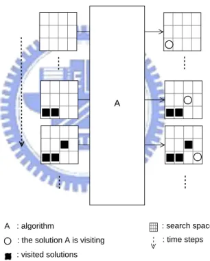
A : algorithm
: visited solutions : the solution A is visiting
A
: search space : time steps
Figure 2.1: An illustration of an algorithm
Definition 4. The search process of A on f , S(A, f ), is the stochastic process (Xi, Yi :=
f (Xi)) over X × Y defined by X1 ∼ AT0 and Xk+1 ∼ A((Xi,Yi))k1. Let S(A, f, k) := ((Xi, Yi))k1, and Sy(A, f, k) := (Yi)k1 is called the performance vector.
Definition 5. Let V :=S|X |i=1Yi be the set containing all possible performance vectors. A
The terminology mostly follows those adopted in [2] and [9] with a few slight mod-ifications applied to avoid the situation that an algorithm is undefinable on a complete trace and to make search processes able to be expressed in a naturally stochastic way. Even though the NFL framework does exert constraints upon the scope of optimization algorithms and problems so that rigorous analysis can proceed, these conditions are not unreasonable for the theorem’s intent. Most general-purpose optimizers, equipped with-out problem-specific knowledge, are essentially black-box algorithms, and the finiteness of the search space agrees with the nature of computer.
Example 1 demonstrates how to represent random search under the NFL framework. It is noteworthy that the non-revisiting property confines random search to the scope of random permutation.
Example 1 (Random search in NFL). Let RTm be a random variable that P rob{RTm = x} = 1/(|X |−m) for all x /∈ Tm. In the NFL framework, random search can be accordingly
defined as RS := {RT | T ∈ T|X |−1}.
2.2
NFL Theorem
Now, the NFL theorem can be given as Theorem 1.
Theorem 1 (NFL theorem). If v ∈ V is a performance vector with length `, then X
f
P rob{Sy(A, f, `) = v} = c ,
where c is a constant independent of A.
The complete proof can be found in the original NFL papers [1, 2]. Also, both Droste et al. [5] and Culberson [3] provide simplified proofs.
To rephrase the NFL theorem more plainly, for any performance vector, the expected number of problems on which the performance vector will be generated in the search process is identical for all algorithms. Since the performance measure is a function defined on performance vectors, for any given “score”, the expected number of problems on which the score is achieved is exactly the same for all algorithms. Therefore, averaging over all problems, all algorithms performs identically in expectation.
Chapter 3
Discrete Lipschitz Class
3.1
Definition of the Discrete Lipschitz Class
In real analysis, Lipschitz functions refer to the functions with bounded slope. Given a set C ⊆ R, f : C → R is a Lipschitz function if there exists a constant K > 0 such that
|f (a) − f (b)| ≤ K|a − b| for all a, b ∈ C. The Lipschitz condition is a stronger condition
than normal continuity, because any Lipschitz function is uniformly continuous. On the other hand, the functions that are not everywhere differentiable may still be Lipschitz, e.g., f (x) = |x|. On a closed interval, the Lipschitz class lies between continuous functions and the functions having continuous derivatives [10].
For the discrete space, there is no such thing as continuity. However, if there is some sort of distance defined in some discrete space, the Lipschitz condition can still be applied, and therefore a natural way to simulate continuity in the discrete space can be obtained. In combinatorics, the spatial structures are typically formed via graph theory. If we view the vertex set as the search space and the edge set as the specification of the geometry, the Lipschitz condition can be transferred here by restricting the difference of objective values between any two adjacent vertexes. The merit of such definition is that we do not put any constraints on the global structure directly such as to demand the functions to be polynomial or the description length to be bounded. Instead, we only expect some similarities of the objective values within a neighborhood in the search space.
Since we will focus on the discrete Lipschitz class in the remainder of this paper, the domain X is always the vertex set V (G) of a graph G, representing the spatial structure. Hence, the two notations X and V (G) are used exchangeably. The discrete Lipschitz class
(DLC) can now be introduced.
Definition 6 (Discrete Lipschitz class, DLC). Given a connected graph G and a finite
set Y ⊂ R, the corresponding discrete Lipschitz class with Lipschitz constant K is defined as
L(G, Y, K) := {f : V (G) → Y | ∀v1v2 ∈ E(G), |f (v1) − f (v2)| ≤ K} .
Throughout this thesis, the property of Y of interest is the ordering, so, without loss of generality, Y is assumed to be a subset of N of the form {0, 1, . . . , m} unless specified otherwise. deg(v) and N(v) are used to denote the degree and the neighborhood of a vertex v, respectively.
3.2
DLC as Representation
In this section, we discuss the connection between DLC and real-world optimization prob-lems in order to manifest the broadness and the practicality of DLC.
3.2.1
Real-parameter Optimization Problems
The definition of DLC provides a means to represent the intrinsically real-parameter optimization problems through discretization (for practical computing devices). For in-stance, if a cube C ⊂ Rn is discretized uniformly into a set of grid points, V (G) =
{x1, x2, . . . , xM}n ⊂ Rn with xi+1 − xi = u > 0, we can let E(G) = {vivj | vi, vj ∈
V (G) and kvi− vjk1 = u}. L(G, Y, K) then forms a class containing all functions, defined
on C with the absolute values of partial derivatives upper bounded by K/u, discretized over V (G). Furthermore, since Y is bounded, this class contains all functions mapping
V (G) to Y with sufficient large K (e.g., K = max Y − min Y).
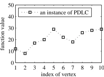
The simplest case of DLC is the class of functions defined on R, in which the graph representing the spatial structure is a simple path. Figure 3.1 gives an illustrative example of such functions.
Definition 7 (Pathwise discrete Lipschitz class, PDLC). Given a finite set Y ⊂ R and a
simple path G = v1v2. . . vn, the pathwise discrete Lipschitz class with Lipschitz constant
1
2
3
4
5
6
7
8
9
10
0
10
20
30
40
50
index of vertex
function value
an instance of PDLC
Figure 3.1: A function instance of PDLC with 10 vertexes and K = 10.
Higher-dimensional cases can be defined in a similar way and will be addressed later in Chapter 6.
3.2.2
Combinatorial Optimization Problems
Since DLC is discrete in nature, if a combinatorial problem can be represented by a solution-based form, then we can characterize it as DLC by specifying the neighborhood structure and the Lipschitz constant. For instance, the search space of the Traveling Salesman Problem(TSP)[11] consists of all possible tours, i.e. Hamiltonian cycles, and for each tour there is a corresponding edge set containing all edges the tour passes through. Therefore, we can define the neighborhood of a tour as the set of tours which agree on all but two edges with the original path, and the Lipschitz constant can be written in terms of the maximum weight, as shown in the following example:
Example 2 (TSP and DLC). If the weights of edges are non-negative and upper-bounded
by a constant K, then every traveling salesman problem is an instance of L(G, Y, 2K), where each vertex of G corresponds to a tour in the original graph and if two tours differ in only two edges, they are considered neighbors.
Note that G is not the original graph on which the TSP defined.
Also, the minimum spanning tree(MST) problem[11] can be associated to DLC simi-larly.
Example 3 (MST and DLC). If the weights of edges are non-negative and upper-bounded
by a constant K, then every MST problem is an instance of L(G, Y, 2K), where each vertex of G corresponds to a spanning tree in the original graph and if two spanning trees differ in only two edges, they are considered neighbors.
In addition to graph problems, the optimization version of the set-partition problem[11], which is to partition a set into two equally weighted subsets, can also be connected to DLC. For a set S ⊂ N, we denote the sum of elements in S as MS, i.e.
P
x∈Sx = MS.
Example 4 (Set-partition problem and DLC). Given a finite set S ⊂ N with max S = K,
the solution space of the set-partition problem is the power set of S. For a subset U of S, the corresponding objective value is f (U) = |MU − MS/2|. Two subsets A and B of
S, where A ⊂ B, are considered neighbors if |B − A| = 1, and thus f (A) ≤ f (B) = |MB− MA+ MA− MS/2| ≤ f (A) + |MA− MB| ≤ f (A) + K. Therefore, the set-partition
problem on S is an instance of DLC with Lipschitz constant K.
Generally speaking, if a combinatorial optimization problem involves a weight set, then normally it can be transformed into DLC. In the following section, we will show that mostly the NFL theorem does not hold over DLC, so it is possible to contrive an algorithm outperforming random search on these combinatorial problems.
3.3
DLC and NFL
In this section, we will investigate DLC within the NFL framework and derive a condition under which the the NFL theorem holds. In order to determine whether the NFL theorem holds over a problem class, Schumacher et al. [9] provided a criterion for the NFL theorem based on permutation closure.
Definition 8 (Permutation closure). If π is a permutation on X , define fπ as fπ(x) :=
f (π(x)) for all x ∈ X . F ⊆ FX ,Y is closed under permutation if for all f ∈ F and for
every permutation π on X , fπ ∈ F .
Although in [9], this criterion is proposed for deterministic algorithms, since a random-ized algorithm is simply a mixed strategy, i.e., a distribution over all possible deterministic strategies [12, 5], this criterion still holds for randomized algorithms in the sense of ex-pectation. Utilizing Lemma 1, a simple criterion for whether or not the NFL result can be applied to a DLC can be obtained.
Theorem 2 (Criterion for NFL on DLC). Let L(G, Y = {0, 1, . . . , m}, K) with m > K
be a DLC. NFL holds over L(G, Y, K) if and only if G is complete.
Proof. By Lemma 1, it is sufficient to show that L(G, Y, K) is closed under permutation
if and only if G is complete.
• If G is complete, for every f ∈ L(G, Y, K), we have |f (vi) − f (vj)| ≤ K for all
vi and vj ∈ V (G). For any permutation π on X and for all vi and vj ∈ V (G),
|fπ(vi) − fπ(vj)| = |f (π(vi)) − f (π(vj))| ≤ K. Therefore, fπ ∈ L(G, Y, K).
• If L(G, Y, K) is closed under permutation, suppose for contradiction that G is not
complete. The incompleteness and connectivity of G imply that there exist vi and
vj ∈ V (G) with vivj ∈ E(G). Select v/ k ∈ N(vi), where N(vi) is the neighborhood
of vi. Obviously, vk 6= vj. Consider the function f ∈ L(G, Y, K):
f (v) = 0 if v = vi ; K + 1 if v = vj ; K otherwise. and the permutation π:
π(v) = vk if v = vj ; vj if v = vk ; v otherwise. |fπ(vk)−fπ(vi)| = |f (π(vk))−f (π(vi))| = |f (vj)−f (vi)| = K+1, so fπ ∈ L(G, Y, K),/ a contradiction.
The completeness of a graph implies that the entire search space is in the same neigh-borhood. However, such a case is rare in real-world applications, because the degree can be viewed as an indication of dimensions, and the size of search space typically surpasses the number of dimensions significantly. For example, for discretized real-parameter optimiza-tion problems, the cardinality of the domain is usually notably larger than the number of dimensions, and hence the corresponding graphs are not complete in most cases. Taking PDLC as an example, when m > K, the NFL theorem sustains over a PDLC only if there are merely two vertexes in the problem.
Chapter 4
DLC and Subthreshold-seeker
The subthreshold-seeker (STS), introduced by Whitley and Rowe [8] and proved to outper-form random search on unioutper-formly sampled polynomials of one variable, is a metaheuristic that employs the threshold as a switch of local search. In essence, it is a selective local search method as it conducts local search if a given condition is satisfied. In this section, a generalization of subthreshold-seeker is firstly presented, and we will demonstrate that the generalized subthreshold-seeker can outperform random search on DLC.
4.1
Generalized Subthreshold-seeker
In Whitley and Rowe’s work, the subthreshold-seeker is an optimization algorithm aiming at functions with a one-dimensional domain, i.e., functions defined on a subset C ⊆ R. The subthreshold-seeker will successively select a point from the search space uniformly at random (u.a.r.) until a subthreshold point is encountered. Once encountering a sub-threshold point, the subsub-threshold-seeker will search through the quasi-basin where that subthreshold point resides. In Whitley and Rowe’s definition, a quasi-basin is a set of contiguous points with objective values below the threshold. In other words, the threshold is used to determine whether the subthreshold-seeker enters the local search phase, and the subthreshold-seeker can be viewed as an optimizer with an exhaustively local search operator.
According to this point of view, we generalize the subthreshold-seeker to the extent that it is applicable to any function of which the domain possesses a neighborhood struc-ture as in Algorithm 1.
Algorithm 1 (Generalized subthreshold-seeker).
procedure Subthreshold-seeker(X , Y, N : X → 2X, f : X → Y)
while the stopping criterion is not satisfied do if Queue is not empty then
x ← Queue.pop(); else
Select x from X u.a.r. end if if f (x) ≤ θ then Queue.push(N(x)) end if end while end procedure
Following the NFL framework, the parts of selecting and pushing are both restricted to unvisited points. Such a task can be achieved by a bookkeeping manner. Since the performance of an algorithm is judged by the performance vector, all overheads other than function evaluations will not count under the NFL framework.
The only control parameter of the subthreshold-seeker is the threshold. The elegance of the subthreshold-seeker is that it comprises the two fundamental operations of search heuristics, local search and global restart, and yet still stays in a simple form.
4.2
Subthreshold-seeker on DLC
Christensen and Oppacher [7] defined the performance measure as the number of subme-dian points visited by an algorithm, and Whitley and Rowe [8] generalized this notion to any threshold less than or equal to the median. That is, given a predefined stopping time
L and α ∈ (0, 1/2], the performance measure is the number of points visited in the first L function evaluations with the top α|X | values in the objective space.
This performance measure may seem odd at the first glance, for typically the perfor-mance of an optimizer is measured in terms of the time in which the optimum is located. However, even focusing on functions as simple as unimodal functions that are monotone with respect to the distance from the optimum, the time complexity analysis is still a difficult task. For instance, to the best of our limited knowledge, the time complexity of (1+1)-ES [13] on such functions has not been analyzed until recently [14]. Hence, it seems unlikely to analyze the runtime of an algorithm that is more sophisticated than random search over a broad class of problems. Furthermore, as mentioned in Chapter 2, within the NFL framework, the performance measure can be any function defined on the set containing all performance vectors, and roughly speaking, with more subthreshold points visited, it is more likely to identify a point with a satisfiable objective value. Therefore, Whitley and Rowe’s notion appears in between theoretically analyzable and practically meaningful.
For any function f , we define βα(f ) be the maximum objective value below the
per-formance threshold, i.e.,
βα(f ) := max ( y ∈ Y ¯ ¯ ¯ ¯ ¯ y X i=0 |{x ∈ X | f (x) = i}| ≤ α|X | ) .
If the set following the “max” notation is empty, then βα(f ) is defined to be −∞. Let
Ψα,f(v) be a performance measure that maps a performance vector v to the number of
components of v below performance threshold, i.e., Ψα,f((v1, v2, . . . , vL)) = |{vi | vi ≤
βα(f )}|. It is noteworthy that the performance threshold should be distinguished from
the algorithmic threshold. The latter should be regarded as a control parameter of the algorithm and hence is not related to the performance measure.
Whitley and Rowe showed that if f is a uniformly sampled polynomials of one vari-able, and βα(f ) is known in advance, setting θ = βα(f ), under certain conditions the
subthreshold-seeker outperforms random search on f . In this thesis, we will show that the subthreshold-seeker with θ within some range of codomain, rather than a specific value, will outperform random search in the sense that for all functions in the DLC, the expected number of points below the performance threshold visited by the subthreshold-seeker is greater than or equal to that by random search, and there does exist a function
such that the inequality is strict.
Theorem 3 (Equal or better performance of STS on DLC). Let L(G, Y = {0, 1, . . . , m}, K)
with m > K be a DLC. For all f ∈ L(G, Y, K) if the algorithmic threshold θ of a subthreshold-seeker satisfies θ ≤ βα(f ) − K, then
E[Ψα,f(Sy(ST S, f, L))] ≥ E[Ψα,f(Sy(RS, f, L))]
for all L with 1 ≤ L ≤ |X |.
Proof. Let f be any function belonging to L(G, Y, K). Suppose S(ST S, f, L) = ((Xsi, Ysi))Li=1
and S(RS, f, L) = ((Xri, Yri))Li=1. Define the indicator variable Isi as Isi = 1 when
Ysi ≤ βα(f ) and Isi = 0 otherwise, and Iri is defined in a similar way for random search.
We can obtain that Ψα,f(Sy(ST S, f, L)) =
PL
i=1Isi and Ψα,f(Sy(RS, f, L)) =
PL
i=1Iri.
We prove the theorem by induction on L. Let U := |{x ∈ V (G) | f (x) ≤ βα(f )} be
the total number of points below the performance threshold. When L = 1, since both strategies select a point u.a.r. from X in the first move, clearly E[Is1] = U/|X | = E[Ir1].
Suppose E[PLi=1Isi] ≥ E[
PL
i=1Iri] for 1 ≤ L < |X |. Then,
E[ L+1 X i=1 Isi] = E[ L X i=1 Isi] + E[IsL+1] (4.1) = E[ L X i=1 Isi] + X (xi)Li=1∈XL E£IsL+1 | (Xsi)Li=1= (xi)Li=1 ¤
P rob{(Xsi)Li=1 = (xi)Li=1}
If Xsi is popped out from the queue, f (Xsi) ≤ θ + K ≤ βα(f ) − K + K = βα(f ),
and hence, Isi = 1. Otherwise, if Xsi is selected from X u.a.r., then P rob{Isi = 1} =
(U − k)/(|X | − i + 1), where k is the number of points visited in the first i − 1 steps with objective values smaller than or equal to βα(f ). Let CL be the set collecting all
move. Therefore, X
(xi)Li=1∈XL
E£IsL+1| (Xsi)Li=1 = (xi)Li=1
¤
P rob{(Xsi)Li=1= (xi)Li=1}
= X
(xi)Li=1∈CL
E[IsL+1 | (Xsi)Li=1∈ CL]P rob{(Xsi)Li=1= (xi)Li=1}+
X
(xi)Li=1∈C/ L
E[IsL+1 | (Xsi)Li=1∈ C/ L]P rob{(Xsi)Li=1 = (xi)Li=1}
= X
(xi)Li=1∈CL
1 · P rob{(Xsi)Li=1 = (xi)Li=1}+ (4.2)
X (xi)Li=1∈C/ L U −¯¯{xi ∈ (xi)Li=1| f (xi) ≤ βα(f )} ¯ ¯ |X | − L P rob{(Xsi) L i=1 = (xi)Li=1} ≥ X (xi)Li=1∈XL U −¯¯{xi ∈ (xi)Li=1| f (xi) ≤ βα(f )} ¯ ¯ |X | − L P rob{(Xsi) L i=1= (xi)Li=1} = L X k=0 U − k |X | − LP rob{ L X i=1 Isi = k} Substituting into (4.1), E[ L+1 X i=1 Isi] ≥ L X k=0 kP rob{ L X i=1 Isi = k} + L X k=0 U − k |X | − LP rob{ L X i=1 Isi = k} = U |X | − L + |X | − L − 1 |X | − L L X k=0 kP rob{ L X i=1 Isi = k} = U |X | − L + |X | − L − 1 |X | − L E[ L X i=1 Isi] ≥ U |X | − L + |X | − L − 1 |X | − L E[ L X i=1 Iri] (4.3) = L X k=0 kP rob{ L X i=1 Iri = k} + L X k=0 U − k |X | − LP rob{ L X i=1 Iri = k} = E[ L X i=1 Iri] + L X k=0 E[IrL+1 | L X i=1 Iri = k]P rob{ L X i=1 Iri = k} = E[ L+1 X i=1 Iri]
Inequality (4.3) follows from the induction hypothesis.
Furthermore, next theorem guarantees that for any f ∈ L(G, Y, K), if there exists a point above performance threshold and the subthreshold-seeker ever enters the local
search phase, the subthreshold-seeker will outperform random search strictly in expecta-tion according to the performance measure Ψα,f.
Theorem 4 (Strictly better performance of STS on DLC). Let L(G, Y = {0, 1, . . . , m}, K)
with m > K be a DLC. For all f ∈ L(G, Y, K) and for every subthreshold-seeker ST S with θ ≤ βα(f ) − K satisfy:
1. ∃v ∈ V (G) with f (v) > βα(f ), and
2. ∃v ∈ V (G) with f (v) ≤ θ,
E[Ψα,f(Sy(ST S, f, L))] > E[Ψα,f(Sy(RS, f, L))] for all L ∈ [2, |X | − 1].
Proof. If there are no such functions in L(G, Y, K), the theorem holds vacuously.
Oth-erwise, let f be any function satisfying the two conditions and define ((Xsi, Ysi))Li=1,
((Xri, Yri))Li=1, Isi, Iri, U, and CL in the same way as in Theorem 3. We prove by
in-duction on L. When L = 2, since in the second step, the queue is nonempty if and only if f (Xsi) ≤ θ, C1 = {v ∈ V (G) | f (v) ≤ θ} 6= ∅ by Condition (2). Therefore, E[Is1+ Is2] =E[Is1] + X x∈X E[Is2 | Xs1 = x]P rob{Xs1 = x} =E[Is1] + X x:f (x)≤θ 1 · P rob{Xs1 = x} + X x:θ<f (x)≤βα(f ) U − 1 |X | − 1P rob{Xs1 = x} + X x:f (x)>βα(f ) U |X | − 1P rob{Xs1 = x} >E[Is1] + X x:f (x)≤βα(f ) U − 1 |X | − 1P rob{Xs1 = x} + X x:f (x)>βα(f ) U |X | − 1P rob{Xs1 = x} =E[Is1] + X k∈{0,1} U − k |X | − 1P rob{Is1 = k} =E[Ir1] + X k∈{0,1} U − k |X | − 1P rob{Ir1 = k} =E[Ir1+ Ir2]
The inequality follows from C1 6= ∅ and (U − 1)/(|X | − 1) < 1, for Condition (1) implies
U < |X |. For induction hypothesis, suppose E[PLi=1Isi] > E[
PL
L < |X | − 1. In the (L + 1)-th step, from the proof of Theorem 3, we always have E[ L+1 X i=1 Isi] ≥ U |X | − L + |X | − L − 1 |X | − L E[ L X i=1 Isi] > U |X | − L + |X | − L − 1 |X | − L E[ L X i=1 Iri] (4.4) = E[ L+1 X i=1 Iri]
Since (|X | − L − 1)/(|X | − L) > 0 when L < |X | − 1, and E[PLi=1Isi] > E[
PL
i=1Iri] from
the induction hypothesis, Inequality (4.4) is strict.
Let d := max{deg(v) | v ∈ V (G)} be the maximum degree of the graph and dis(u, v) be the length of the shortest path from u to v. For any subthreshold-seeker, if we are able to set its θ within some interval, the following corollary gives a sufficient condition of the existence of functions on which the subthreshold-seeker strictly outperforms random search.
Corollary 1. Let L(G, Y = {0, 1, . . . , m}, K) be a DLC. Given α ∈ (0, 1/2] and an
integer C > 1 with CK + 1 ≤ m, if
α|V (G)| > d(d − 1)
C− 2
d − 2 ,
then there exists a function f ∈ L(G, Y, K) such that
E[Ψα,f(Sy(ST S, f, L))] > E[Ψα,f(Sy(RS, f, L))]
for all L with 2 ≤ L ≤ |X | − 1, where ST S is a subthreshold-seeker with θ ∈ βα(f ) −
[K, CK].
Proof. We prove this corollary constructively. Select a vertex v0 from V (G) arbitrarily.
Consider the function f defined as
f (v) = 0 if v = v0 ; dis(v, v0)K if 1 ≤ dis(v, v0) ≤ C ; CK + 1 otherwise.
Since |vo| + |{v ∈ V (G) | 1 ≤ dis(v, v0) ≤ C}| ≤ 1 +¡d + d(d − 1) + d(d − 1)2 + . . . + d(d − 1)C−1¢ = 1 + d £ (d − 1)C − 1¤ (d − 1) − 1 = d(d − 1)C − 2 d − 2 < α|V (G)| ,
from the definition of βα(f ), βα(f ) = CK. Furthermore, there must exist v1 ∈ V (G) that
f (v1) = CK + 1, for |vo| + |{v ∈ V (G) | 1 ≤ dis(v, v0) ≤ C}| < |V (G)|. Therefore, we
have f (v0) ≤ θ and f (v1) > βα(f ). Thereby Theorem 4 can be applied.
Combining Theorem 3 and Theorem 4, if we manage to set θ ≤ βα(f ) − K, the
subthreshold-seeker will perform at least as good as random search on a DLC. If the subthreshold-seeker has a chance to conduct local search, it will strictly outperform ran-dom search. Estimating a θ within some range should be more practical than gauging a specific value such as βα(f ). In next section, we will explore this possibility and
empiri-cally confirm the theoretical results obtained in this section by proposing and adopting a sampling-test scheme.
Chapter 5
Sampling-test Scheme for PDLC
Conventionally, the effectiveness of an optimizer is examined via experiments on a suite of test functions that serves as a benchmark. These test functions are selected according to some prior knowledge of the importance thereof. Here we propose and adopt a different approach in order to confirm the theoretical results obtained in the previous section from an empirical aspect. We draw a sample of functions randomly from PDLC in a manner similar to select respondents in a campaign survey and conduct experiments on these sampled functions. There is no bias in favor of which functions should be selected. We expect the arbitrariness delivers information about the composition of the problem class. A uniform sampler for PDLC is firstly given in Section 5.1. Experiments are then pre-sented to summarize this section and demonstrate how the Lipschitz condition facilitates the search process in a practical standpoint.
5.1
A Uniform Sampler for PDLC
In order to conduct the sampling test, we need a uniform sampler in the first place. The following algorithm generates problem instances of PDLC with Lipschitz constant K uni-formly at random (u.a.r.)
Algorithm 2 (Uniform PDLC Sampler).
procedure Uniform PDLC Sampler(v1v2. . . vn, Y = {0, 1, . . . , m}, K)
f (v1) ← Unif orm([0, m])
while i ≤ n do
f (vi) ← f (vi−1) + Unif orm([−K, K])
i ← i + 1 if f (vi) > m or f (vi) < 0 then f (v1) ← Unif orm([0, m]) i ← 2; end if end while return f end procedure
Remark 1. The sequence of objective values, f (vi), forms a martingale.
Here Unif orm([a, b]) denotes the function that selects an integer u.a.r. from the closed interval [a, b]. Such a sampler belongs to the category of accept-reject algorithms [15]. It generates a problem instance with bounded difference between any two successive vertexes u.a.r., and if the instance at hand exceeds the range of the codomain, the sampler rejects the instance. The accept-reject mechanism guarantees the uniformity. Once the sampler halts, the output is always an instance of the PDLC.
Since this sampler is Las Vegas, we need to address its time complexity for the prac-ticality. For each candidate instance, the sampler will go through at most |X | steps to assign all the vertex objective values, so it remains to show how many candidate instances it takes to generate a legit instance successfully. The accept-reject process is geometrically distributed, and therefore the expected number of instances consumed is the inverse of the acceptance probability. The following theorem provides an upper bound for the rejection probability.
Lemma 2. Suppose |Y| = 2m + 1, where m is an integer, and |X | = n. If
m >
r
(n − 1)(K2+ K)
3 ≥ 2 ,
then the rejection probability is less than
4p(n − 1)(K2+ K) √ 3|Y| − 4(n − 1)(K2+ K) 3|Y|2 + 5 |Y| .
Proof. Without loss of generality, suppose Y = {−m, −m + 1, . . . , m}. Let (Ki) be a
sequence of i.i.d. random variables that Ki = j with probability 1/(2K + 1) for j ∈
{−K, −K + 1, . . . , K} and Sj :=
Pj
i=1Ki. When f (v1) = i, the instance is rejected if
and only if i + Sj ≥ m + 1 or i + Sj ≤ −m − 1 for some 1 ≤ j ≤ n − 1, so the occurrence
of rejection always implies max1≤j≤n−1|Sj| ≥ min{|m + 1 − i|, | − m − 1 − i|}. Moreover,
the symmetry indicates that P rob{rejection | f (v1) = i} = P rob{rejection | f (v1) = −i}
for |i| ≤ m. Therefore,
P rob{rejection}
=
m
X
i=−m
P rob{rejection | f (v1) = i}P rob{f (v1) = i}
= Pm i=−mP rob{rejection | f (v1) = i} 2m + 1 ≤ P rob{max1≤j≤n−1|Sj| ≥ m + 1} + 2 Pm i=1P rob{max1≤j≤n−1|Sj| ≥ m + 1 − i} 2m + 1 = P rob{max1≤j≤n−1|Sj| ≥ m + 1} + 2 Pm i=1P rob{max1≤j≤n−1|Sj| ≥ i} 2m + 1 .
Using Kolmogorov’s inequality [16], we can get
P rob{ max 1≤j≤n−1|Sj| ≥ i} ≤ min ½ V ar[Sn−1] i2 , 1 ¾ .
Since V ar[Ki] = 2(12 + 22 + . . . + K2)/(2K + 1) = (K2 + K)/3, V ar[Sn−1] = (n −
1)V ar[Ki] = (n − 1)(K2 + K)/3. Moreover, V ar[Sn−1]/i2 ≤ 1 if and only if i ≥
p V ar[Sn−1], we have P rob{rejection} ≤ V ar[Sn−1] (m+1)2 + 2 µ Pl√V ar[Sn−1] m −1 i=1 1 + Pm i=l√V ar[Sn−1] m V ar[Sn−1] i2 ¶ 2m + 1 ≤ V ar[Sn−1] (m+1)2 + 2 µlp V ar[Sn−1] m − 1 + V ar[Sn−1] Rm x=l√V ar[Sn−1] m −1x −2dx ¶ 2m + 1 ≤ V ar[Sn−1] (m+1)2 + 2 µp
V ar[Sn−1] −V ar[Smn−1] +l√V ar[Sn−1] V ar[Sn−1]
m
−1
¶
Since x/(x − 1) decreases when x > 1, we obtain V ar[Sn−1] lp V ar[Sn−1] m − 1 ≤ V ar[Sn−1] p V ar[Sn−1] − 1 =pV ar[Sn−1] + p V ar[Sn−1] p V ar[Sn−1] − 1 ≤pV ar[Sn−1] + 2 .
According to the hypothesis that V ar[Sn−1]/(m + 1)2 < 1,
P rob{rejection} < 4 p V ar[Sn−1] − 2V ar[Smn−1] + 5 2m + 1 = 4 p (n − 1)(K2+ K) √ 3(2m + 1) − 2(n − 1)(K2+ K) 3m(2m + 1) + 5 2m + 1 < 4 p (n − 1)(K2+ K) √ 3|Y| − 4(n − 1)(K2+ K) 3|Y|2 + 5 |Y| .
Theorem 5 (Upper bound for the rejection probability). Define m := b(|Y| − 1)/2c. If
m >p(n − 1)(K2+ K)/3 ≥ 2 , then the rejection probability is less than
4p(n − 1)(K2+ K) √ 3|Y| − 4(n − 1)(K2+ K) 3|Y|2 + O ¡ |Y|−1¢ .
Proof. If |Y| = 2m + 1, then we are done by the previous lemma. Otherwise, if |Y| =
2m + 2, without loss of generality, suppose that Y = {−m, −m + 1, . . . , m + 1} and let
Y0 = {−m, −m + 1, . . . , m}. Therefore, P rob{rejection} =P rob{f (v1) ∈ Y0}P rob{rejection | f (v1) ∈ Y0} + P rob{f (v1) /∈ Y0}P rob{rejection | f (v1) /∈ Y0} = µ 2m + 1 2m + 2 ¶ P rob{rejection | f (v1) ∈ Y0} + µ 1 2m + 2 ¶ P rob{rejection | f (v1) = m + 1} .
When f (v1) ∈ Y0, if f exceeds the range of Y, then f also exceeds the range of Y0, so
from the previous lemma we have
P rob{rejection | f (v1) ∈ Y0} < 4p(n − 1)(K2+ K) √ 3(2m + 1) − 4(n − 1)(K2+ K) 3(2m + 1)2 + 5 2m + 1 .
As a result, P rob{rejection} ≤ µ 2m + 1 2m + 2 ¶ P rob{rejection | f (v1) ∈ Y0} + µ 1 2m + 2 ¶ < 4 p (n − 1)(K2+ K) √ 3(2m + 2) − 4(n − 1)(K2+ K) 3(2m + 1)(2m + 2) + 6 2m + 2 < 4 p (n − 1)(K2+ K) √ 3|Y| − 4(n − 1)(K2+ K) 3|Y|2 + O ¡ |Y|−1¢
Corollary 2. If |Y| = Cp(n − 1)(K2+ K) > C · 2√3 for some constant C ≥ √3, then
the rejection probability is less than
4√3C − 4 3C2 + O ¡ |Y|−1¢ . Proof. If C ≥√3, m = ¹ |Y| − 1 2 º ≥ |Y| 2 − 1 ≥ p 3(n − 1)(K2+ K) 2 − 1 = r (n − 1)(K2+ K) 3 + p (n − 1)(K2+ K) 2√3 − 1 > r (n − 1)(K2+ K) 3 .
Substituting p(n − 1)(K2+ K)/|Y| by 1/C and applying Theorem 5, the corollary is
proved.
For instance, if C = √3 and |Y| is so large that O(|Y|−1) is negligible, the expected number of instances consumed is no more than 9. Multiplying the time to assign all vertexes values, the expected runtime, in terms of the number of assignments, is no more than 9|X |. In other words, asymptotically speaking, if |X | and |Y| are about equal and
|Y| is larger than K2 to some extent, then the expected runtime is approximately linear.
5.2
Experimental Settings and Results
As demonstrated in Chapter 4, the virtues of the subthreshold-seeker rely on a proper algorithmic threshold. Although the main results in Chapter 4 hold when θ ≤ β (f ) − K,
because we do not set a performance threshold literally to scrutinize how many sub-threshold points are visited in real-world applications, in an experimental setting, we can examine the subthreshold-seeker more practically in terms of the time to identify the op-timum. Therefore, the algorithmic threshold should be utilized for optimization, or more specifically, to minimize the objective function in this case.
We will compare the subthreshold-seeker with random search. Here we present three different subthreshold-seekers. For the theoretical purpose, the first one uses the actual median of all objective values, in the form of exterior knowledge, as θ. The second one firstly selects a 100 points u.a.r. and then employs the calculated median as θ. The third one also starts with obtaining 100 points u.a.r., but it computes the mean and the standard deviation of these points and sets θ to the mean minus the standard deviation. Moreover, the three subthreshold-seekers and random search obey the NFL framework and hence are non-repeating.
In advance of experiments, we need to determine the size of the set PDLC problems to be sampled. Suppose we want to estimate a population proportion q ∈ [0, 1]. We draw a sequence of samples uniformly and independently from the population with replacement. For each sample, we observe if it belongs to the variety of interest. With a large sample size, we expect the proportion in the sample approximates the real proportion. The following theorem depicts the relationship between the sample size and the error bound. Theorem 6 (Sample size and error bound). Let (Zi) be a sequence of i.i.d. indicator
variables with E[Zi] = q. For all δ, ² ∈ (0, 1), if
n ≥ −ln(δ/2) 2²2 , then P rob ½¯¯ ¯ ¯ Pn i=1Zi n − q ¯ ¯ ¯ ¯ > ² ¾ ≤ δ .
Proof. Let Z = (Pni=1Zi)/n. Applying Hoeffding’s inequality [17], for 0 < ² < 1 − q, we
have
P rob{Z − q > ²} ≤ e−2n²2
and for 0 < ² < q, P rob{Z − q < −²} ≤ e−2n²2 . Moreover, if ² ≥ 1 − q, P rob{Z − q > ²} ≤ P rob{Z > 1} = 0 ≤ e−2n²2 . Similarly, if ² ≥ q, P rob{Z − q < −²} ≤ P rob{Z < 0} = 0 ≤ e−2n²2 .
Hence, we conclude that for all ² ∈ (0, 1),
P rob{|Z − q| > ²} ≤ 2e−2n²2 . Finally, n ≥ −ln(δ/2) 2²2 implies 2e−2n²2
≤ δ, and we complete the proof.
In particular, with the conventional setting of (², δ) = (0.03, 0.05), a sample of size 2, 050 suffices. In other words, if we draw a sample of size 2, 050, [Z − 0.03, Z + 0.03] forms a confidence interval for q with confidence level at least 95%.
The sampler generates 2,050 instances of PDLC with (|X |, |Y|) = (104, 104), (105, 105),
and (106, 106), respectively. The Lipschitz constant K is set to 100 for the concern of
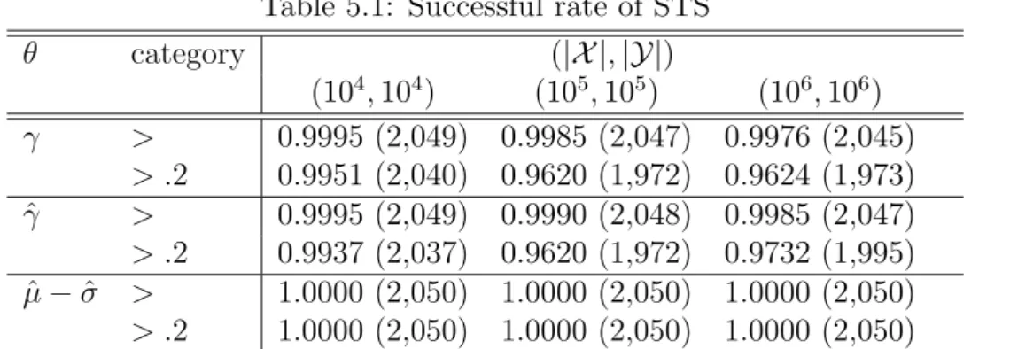
execution time, as previously discussed. For each problem instance, we test each algorithm for 50 independent runs. If the average time of a subthreshold-seeker to find the optimum is less than that of random search, the instance is counted as a success. We also count the number of instances that a subthreshold-seeker outperforms random search by a 20% margin, i.e., the instance where the average optimization time of a subthreshold-seeker is less than 80% of that of random search. Table 5.1 displays the empirical results.
All three subthreshold-seekers outperform random search in most of the sampled prob-lem instances. Furthermore, the subthreshold-seeker with θ = ˆµ − ˆσ outperforms random
search in all 2,050 instances sampled, even with the requirement of a 20% margin. The statistical significance of such results is obvious to see: Suppose the population proportion
Table 5.1: Successful rate of STS θ category (|X |, |Y|) (104, 104) (105, 105) (106, 106) γ > 0.9995 (2,049) 0.9985 (2,047) 0.9976 (2,045) > .2 0.9951 (2,040) 0.9620 (1,972) 0.9624 (1,973) ˆ γ > 0.9995 (2,049) 0.9990 (2,048) 0.9985 (2,047) > .2 0.9937 (2,037) 0.9620 (1,972) 0.9732 (1,995) ˆ µ − ˆσ > 1.0000 (2,050) 1.0000 (2,050) 1.0000 (2,050) > .2 1.0000 (2,050) 1.0000 (2,050) 1.0000 (2,050)
γ: median. ˆγ: estimated median. ˆµ: estimated mean. ˆσ: estimated standard deviation.
”>”: proportion of instances where the subthreshold-seeker outperforms random search. ”> .2”: proportion of instances where the subthreshold-seeker outperforms random search by a 20% margin.
Table 5.2: Mean time steps to locate the minimum
algorithm (|X |, |Y|) (104, 104) (105, 105) (106, 106) STS, θ = γ 2037.58 22913.23 229232.26 STS, θ = ˆγ 2221.44 23170.58 229532.04 STS, θ = ˆµ − ˆσ 918.29 8095.78 80322.92 random search 4972.50 49724.74 496912.49
γ: median. ˆγ: estimated median. ˆµ: estimated mean. ˆσ: estimated standard deviation.
that the subthreshold-seeker with θ = ˆµ − ˆσ outperforms random search is q. To obtain
the result that random search is outperformed in all instances, the probability is q2050.
Even if q is as high as 0.995, the above probability is just 0.000034. To more formally rephrase, if the null hypothesis is “q ≤ 0.995”, the p-value is merely 0.000034.
Table 5.2 displays the averaged optimization time over the 2,050 sampled problem instances. The subthreshold-seeker with θ = ˆµ − ˆσ outperforms others by a significant
margin. Random search averages approximately |X |/2 to find the minimum, which is expected. The subthreshold-seeker using the actual median and the one using the sample median both take about half time steps of that needed by random search to optimize the function.
The subthreshold-seekers with θ = ˆµ − ˆσ and θ = ˆγ are indeed black-box algorithms,
for there is no exterior knowledge exerted and the only information they can use are function evaluations, but they outperform random search by a remarkable difference.
5.3
The Estimation of Median
In this section, we address the issue of the estimation of median as an echo to Section 5.2 section and Corollary 1 in Chapter 4.
The performance difference between θ = ˆγ and θ = γ is insignificant, suggesting that in this case, an estimation of median may be adequate. Suppose that P with |P | = N is a subset of real numbers, and for all i ∈ P , R(i) is defined to be the rank (i.e., ordering) of
i in P . For instance, R(min P ) = 1 and R(max P ) = N. For simplicity, we assume that N is odd and hence the median of P is the element i with R(i) = dN/2e. Now we want
to estimate the median of P . If a point sample S of size n, where n is assumed odd, is drawn by successively selecting an element u.a.r. from P with replacement, the estimated median, γ, is presumed to be the sampled median, and we want the error is bounded by
² > 0, i.e., |R(γ) − dN/2e | ≤ ²N.
If R(γ) < dN/2e−²N , there are at least dn/2e selections with ranks less than dN/2e−
²N. Let Xi be the indicator variable that indicates if the i-th selection is less than
dN/2e − ²N , Xi = 1 with probability p := (dN/2e − b²N c − 1)/N. R(γ) < dN/2e − ²N
if and only if Pni=1Xi ≥ dn/2e. Since E[
Pn
i=1Xi] = np, applying another form of
Hoeffding’s inequality [17], we have
P rob ½ R(γ) < » N 2 ¼ − ²N ¾ = P rob ( n X i=1 Xi ≥ ln 2 m) ≤ P rob ( n X i=1 Xi ≥ n 2 ) = P rob ( 1 n n X i=1 Xi ≥ p + ( 1 2− p) ) ≤ "µ p p + 1 2 − p ¶p+1 2−pµ 1 − p 1 − p − (1 2 − p) ¶1−p−(1 2−p) #n = [4p(1 − p)]n2 . Moreover, the symmetry implies that
P rob ½ R(γ) > » N 2 ¼ + ²N ¾ ≤ [4p(1 − p)]n2 .
Therefore, P rob ½¯¯ ¯ ¯R(γ) − » N 2 ¼¯¯ ¯ ¯ > ²N ¾ ≤ 2 [4p(1 − p)]n2 . Now the only quantity left is p. By definition,
p = §N 2 ¨ − b²Nc − 1 N ≈ 1 2− ² .
For instance, if we set ² = 0.1 and n = 100, the probability of exceeding the error bound is less than 0.26. If the sample size n increases to 2, 000, even with a small ² = 0.03, the probability reduces to just 0.054. It is noteworthy that the effect of the population size
N is negligible. Therefore, the required number of samples remains the same, even if the
search space is immense. Although in real-world applications P is usually a multiset, if the multiplicities of P are not too large, such a gauge should not diverge significantly.
Chapter 6
Toward Higher Dimensions
In this chapter, we attempt to extend the sampling-test scheme proposed in Chapter 5 to higher dimensions and examine a few methods to generate planar DLC, i.e. two-dimensional DLC.
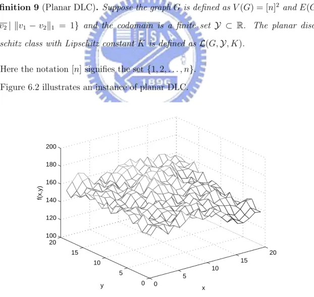
Definition 9 (Planar DLC). Suppose the graph G is defined as V (G) = [n]2 and E(G) =
{v1v2| kv1 − v2k1 = 1} and the codomain is a finite set Y ⊂ R. The planar discrete
Lipschitz class with Lipschitz constant K is defined as L(G, Y, K).
Here the notation [n] signifies the set {1, 2, . . . , n}. Figure 6.2 illustrates an instance of planar DLC.
0 5 10 15 20 0 5 10 15 20 100 120 140 160 180 200 x y f(x,y)
In this chapter, the graph G is defined as V (G) = [n]2 and E(G) = {v
1v2| kv1−v2k1 =
1} unless specified otherwise.
6.1
Accept-reject Sampler for Planar DLC
In this section, we adopt the accept-reject algorithm proposed in Chapter 5 and modify it into an uniform sampler for planar DLC.
Algorithm 3 (Uniform Planar DLC Sampler).
procedure Uniform Planar DLC Sampler(G, Y = {0, 1, . . . , m}, K) Fix a rooted spanning tree T of G
f (root) ← Unif orm([0, m]) for each node v do
f (v) ← f (parent(v)) + Unif orm([−K, K]) end for
if ∃vi, vj ∈ V (G) such that vivj ∈ E(G) and |f (vi) − f (vj)| > K then
Reject and restart end if
if ∃v ∈ V (G) such that f (v) /∈ Y then Reject and restart
end if Return f end procedure
This sampler uniformly generate instances of DLC defined on T , and if the instance at hand is in L(G, Y, K), the sampler will halt and output the instance. In fact, Algorithm 3 can be applied to generate not only planar DLC but also all DLC in general, since the requirement of connectivity in Definition 6 guarantees the existence of a spanning tree.
However, in addition to rejecting out-of-codomain instances, for cyclic graphs, this sampler needs to check additionally that for any edge not in the spanning tree the dif-ference between its two endpoints is less than or equal to K. Therefore, the acceptance probability decreases exponentially with respect to |E(G)| − |E(T )|, which implies that
0 2 4 6 0 2 4 6 850 860 870 880 890 900 x y f(x,y)
Figure 6.2: an instance of planar DLC generated by Algorithm 3
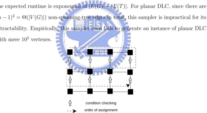
the expected runtime is exponential of |E(G)| − |E(T )|. For planar DLC, since there are (n − 1)2 = Θ(|V (G)|) non-spanning-tree edges in total, this sampler is impractical for its
intractability. Empirically, this sampler even fails to generate an instance of planar DLC with mere 102 vertexes.
order of assignment condition checking
Figure 6.3: the order of assignment and condition checking of a planar DLC sampler
Furthermore, for planar DLC, there exists a Hamiltonian path in G. Therefore, We can arrange the order of vertexes such that the assignment of objective values and condition checking can be done in the same pass, and each vertex only needs to be checked once, as shown in Figure 6.3. That is to say, the generation of planar DLC can be transformed into the generation of PDLC on a Hamiltonian path provided with some overheads of inspecting. Such a result suggests that the number of problems in planar DLC is
signifi-cantly less than that of PDLC. In consequence, to generate planar DLC via the sampler of PDLC appended with further sieving mechanism is infeasible.
Similar to Section 5.2, we examine the performances of subthreshold-seekers and ran-dom search, as shown in Table 6.1 and Table 6.2. The sample size for estimating the algorithmic threshold is 6 for |X | = 62 and 10 for |X | = 72. In spite of the diminutive
search space, the two subthreshold-seekers still outperform random search in above 80% instances sampled.
Table 6.1: Experimental results on planar DLC with |X | = 62,K = 10
algorithm category > > .2 time STS, θ = ˆγ 0.8190(1,679) 0.3346(686) 14.70 STS, θ = ˆµ − ˆσ 0.8015(1,643) 0.3312(679) 14.77 random search 17.02 ˆ
γ: estimated median. ˆµ: estimated mean. ˆσ: estimated standard deviation.
Table 6.2: Experimental results on planar DLC with |X | = 72,K = 10
algorithm category > > .2 time STS, θ = ˆγ 0.8478(1,738) 0.3746(768) 19.74 STS, θ = ˆµ − ˆσ 0.8415(1,725) 0.3956(811) 19.57 random search 23.25 ˆ
γ: estimated median. ˆµ: estimated mean. ˆσ: estimated standard deviation.
6.2
MCMC Sampler
In this section, we turn to the MCMC(Markov chain Monte Carlo) method for sampling. The MCMC method is to design a Markov chain with its stationary distribution equal to the desired distribution [18][15], e.g. uniform distribution in our case.
Algorithm 4 (MCMC Planar DLC Sampler).
procedure MCMC Planar DLC Sampler(G, Y = {0, 1, . . . , m}, K) Initialize f as an arbitrary function f0 ∈ L(G, Y, K)
u.a.r. select v ∈ V (G)
Increment ← Unif orm([−K, K]) if f (v) + Increment ∈ Y then if ∀v0 ∈ N(v), |f (v) + Increment − f (v0)| ≤ K then f (v) ← f (v) + Increment end if end if end while Return f end procedure
Similar to Algorithm 3, this sampler is applicable to all DLC. This algorithm is con-ceived as a Markov chain whose each state is an instance of planar DLC. In other words, it defines a random walk on L(G, Y, K). As time goes to infinity, each state is equally likely to occur, and hence the uniformity is achieved. The following theorem shows that the stationary distribution of this chain is uniform.
Theorem 7. The stationary distribution of the Markov chain defined by Algorithm 4 is
uniform.
Proof. For all fi ∈ L(G, Y, K), we define
N(fi) := {f ∈ L(G, Y, K)| ∃v ∈ V (G) such that |f (v) − fi(v)| ≤ K
and ∀v0 6= v f (v0) = f i(v0)} .
For fi, fj ∈ L(G, Y, K), the transition probability Pfi,fj is
Pfi,fj = 1/(2Kn2) if f j ∈ N(fi) ; 0 if fj ∈ N(f/ i) ; 1 − |N(fi)|/(2Kn2) if fi = fj .
Since this chain is irreducible and aperiodic, from Lemma 10.7 of [18], this theorem is proved.
0 10 20 30 0 10 20 30 80 100 120 140 x y f(x,y)
Figure 6.4: An instance of planar DLC generated by Algorithm 4
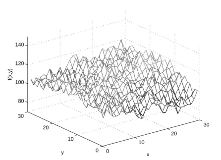
Nevertheless, Theorem 7 only guarantees that this Markov chain will eventually con-verge to uniform distribution, yet it is doubtful that this chain is rapidly mixing when K is much smaller than |V (G)| and |Y|. Figure 6.4 demonstrates an instance generated by Algorithm 4 with |V (G)| = 302, K = 10 and the maximum number of iterations 109, and
it can be observed that the landscape of the solution space is quite level.
6.3
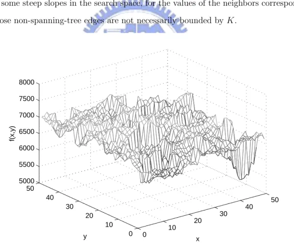
Semi-planar DLC
As demonstrated previously, the practicability of both Algorithm 3 and 4 is questionable for large |V (G)|. Also, the arguments in Section 6.1 suggest that no matter how a sampler assigns values to vertexes, it inevitably fails if the number of edges needing to be checked is enormous. Hence, in order to generate instances with sufficient vertexes, we will loose the restriction of Lipschitz condition slightly to avoid edge checking, so the DLC instances generated here are semi-planar in the sense that they belong to the DLC defined on a spanning tree of G, rather than G itself. More specifically, we will discard the edge-checking mechanism in Algorithm 3 and prefix to it a uniform spanning-tree generater. In other words, the sampler firstly generates a spanning tree u.a.r. and thereafter assign values to vertexes according to it.