立交通大學]
On: 01 May 2014, At: 00:41 Publisher: Taylor & Francis
Informa Ltd Registered in England and Wales Registered Number: 1072954 Registered office: Mortimer House, 37-41 Mortimer Street, London W1T 3JH, UK
Cybernetics and
Systems: An
International Journal
Publication details, including instructions for authors and subscription information: http://www.tandfonline.com/loi/ucbs20
A NEW METHOD FOR
CONSTRUCTING FUZZY
DECISION TREES AND
GENERATING FUZZY
CLASSIFICATION
RULES FROM TRAINING
EXAMPLES
Shyi-Ming Chen, Shih-Yirng Lin a
Department of Electronic Engineering, National Taiwan University of Science and Technology, Taipei, Taiwan, R.O.C. b
Department of Computer and
Information Science, National Chiao Tung University, Hsinchu, Taiwan, R. O. C. Published online: 29 Oct 2010.
To cite this article: Shyi-Ming Chen, Shih-Yirng Lin (2000) A NEW METHOD FOR CONSTRUCTING FUZZY DECISION TREES AND
GENERATING FUZZY CLASSIFICATION RULES FROM TRAINING EXAMPLES, Cybernetics and Systems: An International Journal, 31:7, 763-785, DOI: 10.1080/01969720050192054
To link to this article: http://dx.doi.org/10.1080/01969720050192054
PLEASE SCROLL DOWN FOR ARTICLE
Taylor & Francis makes every effort to ensure the accuracy of all the information (the “Content”) contained in the publications on our platform. However, Taylor & Francis, our agents, and our licensors make no representations or warranties whatsoever as to the accuracy, completeness, or suitability for any purpose of the Content. Any opinions and views expressed in this publication are the opinions and views of the authors, and are not the views of or endorsed by Taylor & Francis. The accuracy of the Content should not be relied upon and should be independently verified with primary sources of information. Taylor and Francis shall not be liable for any losses, actions, claims, proceedings, demands, costs, expenses, damages, and other liabilities whatsoever or howsoever caused arising directly or indirectly in connection with, in relation to or arising out of the use of the Content.
This article may be used for research, teaching, and private study purposes. Any substantial or systematic reproduction, redistribution, reselling, loan, sub-licensing, systematic supply, or distribution in any form to anyone is expressly forbidden. Terms & Conditions of access and use can be found at http:// www.tandfonline.com/page/terms-and-conditions
A NEW M ETHOD FOR CONSTRUCTING FUZZY
DECISION TREES AND GENERATING FUZZY
CLASSIFIC ATION RULES FROM TRAINING
EXAMPLES
SHYI-M ING CHEN
Department of Electronic Engineering,
National Taiwan University of Science and Technology, Taipei, Taiwan, R. O. C.
SHIH- YIRNG LIN
Department of Computer and Information Science, National Chiao Tung University,
Hsinchu, Taiwan, R. O. C.
This paper presents a new method for constructing fuzzy decision trees and generating fuzzy classi¢cation rules from training instances using compound analysis techniques. The proposed method can generate simpler fuzzy classi-¢cation rules and has a better classiclassi-¢cation accuracy rate than the existing method. Furthermore, the proposed method generated less fuzzy classi¢-cation rules.
In recent years, there were many researchers focusing on the research of the inductive learning for rules generation, e.g., Hart (1995), Hunt et al. (1966), Minger (1989), Quinlan (1979, 1986), and Yasdi (1991).
Copyright # 2000 Taylor & Francis 0196-9722/ 00 $12.00 + .00
This work was supported in part by the National Science Council, Republic of China, under Grant NSC 89-2213-E-011-060 .
Address correspondence to Professor Shyi-Ming Chen, Department of Electronic Engineering, National Taiwan University of Science and Technology, Taipei, Taiwan, R.O.C.
763
The extended models using fuzzy set theory (Zadeh, 1965) for fuzzy rules generation can be found in Chang and Pavlidis (1977), Boyen and Wehenkel (1999), Chen and Yeh (1997), Lin and Chen (1996), Sun (1995), Wu and Chen (1999), Yasdi (1991), and Yuan and Shaw (1995). Chang and Pavlidis (1977) presented fuzzy decision tree algorithms. Boyen and Wehenkel (1999) presented a method to fuzzy tree induction from examples for power system security assessment. In Chen and Yeh (1997), the authors have presented a method for generating fuzzy rules from relational database systems for estimating null values by con-structing fuzzy decision trees. In Lin and Chen (1996), the authors have presented a method for generating fuzzy rules from fuzzy decision trees. In Sun (1995) a fuzzy approach to decision trees was presented. In Wu and Chen (1999) the authors have presented a method for con-structing membership functions and fuzzy rules from training examples. Yasdi (1991) presented a method for learning classi¢cation rules from a database in the context of knowledge acquisition and representation. Yuan and Shaw (1995) presented a method for generating fuzzy rules from fuzzy decision trees.
There are some problems with the traditional ID3 learning method (Quinlan, 1986). For example, it cannot deal with cognitive uncertainties (Yuan & Shaw, 1995) such as vagueness and ambiguity associated with human thinking and perception. Furthermore, it is sensitive to ``noise’’ (Sun, 1995). Yuan and Shaw (1995) proposed an algorithm combined with fuzzy logic to solve these problems. However, there are some draw-backs in the method presented in Yuan and Shaw (1995) described as follows:
(1) It takes much computation time to ¢nd the ``entropy’’ of attributes by using a more complex test function.
(2) Yuan and Shaw’s method generated more decision nodes and induced more fuzzy rules.
In this article, a new method for constructing fuzzy decision tree and generating fuzzy rules from training instances was presented, using com-pound analysis techniques. It is a simpler, more ef¢cient, and more effec-tive method, where a simple test function is used to ¢nd the entropy of attributes; instead of using fuzzy subsethood (Sun, 1995), the correctness of classi¢cation is used as the criteria (Jeng & Liang, 1993) to stop the expansion of the fuzzy decision trees. In the process of constructing
764 S.-M. CHEN AND S.-Y. LIN
fuzzy decision trees, the proposed method does not directly ¢nd the entropy of attributes, but tries to ¢nd some factors that are negative to each class. The proposed method can overcome the drawbacks of the one presented in Yuan and Shaw (1995).
BASIC CONCEPTS OF CONSTRUCTING FUZZY DECISION TREES AND GENERATING FUZZY CLASSIFICATION RULES
Quinlan (1986) proposed a learning algorithm called ID3 to construct decision trees from a set of training instances based on information theory. A decision tree is a tree supporting an inference for classi¢cations of all possible instances, where every path from the root to each terminal node forms a rule.
A fuzzy decision tree is an extension of Quinlan’s decision tree. It can avoid unexpected results caused by ``noise,’’ which might take place with a nonfuzzy approach, and it can deal with cognitive uncertainty such as vagueness and ambiguity associated with human thinking and perception.
Before constructing a fuzzy decision tree, one must fuzzify the train-ing data set by applytrain-ing the concepts of fuzzy sets (Chen, 1986; Zadeh, 1965, 1975) and fuzzi¢cation. One can construct a fuzzy decision tree from the training data set and then generate fuzzy classi¢cation rules from the constructed fuzzy decision tree. The objective is to generate a set of fuzzy classi¢cation rules having the following form:
If A is AiAND B is BjTHEN C is Ck …1†
where A and B are attributes of an instance; Ai and Bj are linguistic
terms of A and B, respectively; Ck is a class term of the classi¢cation
attribute C. Then, one can forecast the value of the class term Ck of
the classi¢cation attribute C. Let a and b be membership values of the instance in Aiand Bj, respectively and let c be the forecasted value
of Ck, where c ˆ min(a, b) and ``min’’ is the minimum operator. When
two or more rules have the same conclusion (i.e., they all conclude that ``IF conditions THEN C is Ck’’), then one generates several forecasted
values with respect to Ck, and one takes the largest one.
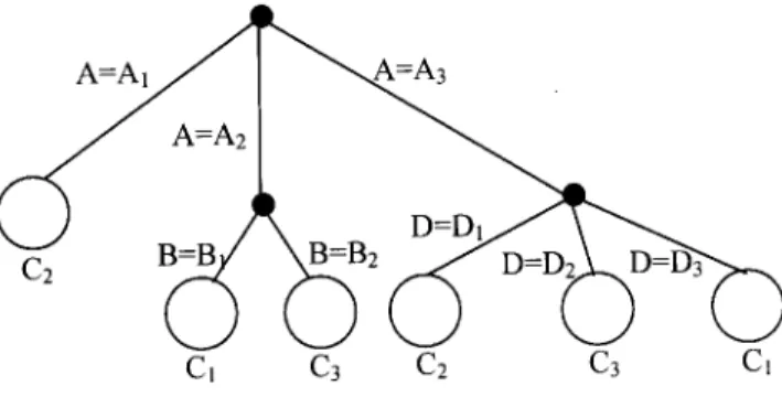
Figure 1 shows an example of a fuzzy decision tree. From Figure 1, one can obtain the fuzzy rules shown as follows:
IF A is A1 THEN C is C2 IF A is A2 AND B is B1 THEN C is C1 IF A is A2 AND B is B2 THEN C is C3 IF A is A3 AND D is D1 THEN C is C2 IF A is A3 AND D is D2 THEN C is C3 IF A is A3 AND D is D3 THEN C is C1 where
(1) C1, C2, and C3 are class terms of the classi¢cation attribute C.
(2) A, B, and D are attributes; A1, A2, and A3are linguistic terms of the
attribute A; B1and B2are linguistic terms of the attribute B; and D1,
D2, and D3 are linguistic terms of the attribute D, respectively.
A NEW M ETHOD FOR CONSTRUCTING FUZZY DECISION TREES AND GENERATING FUZZY RULES
In the following, a new method to generate fuzzy classi¢cation rules is proposed based on constructing fuzzy decision trees using compound analysis techniques. One generalizes the traditional ID3 algorithm (Quinlan, 1986) to deal with cognitive uncertainties such as vagueness and ambiguity associated with human thinking and perception. In addition, combining with fuzzy logic, one can reduce the sensitivity to ``noise.’’ Most important of all one tries to ¢nd in£uential factors that
Figure 1. A fuzzy decision tree.
766 S.-M. CHEN AND S.-Y. LIN
can directly produce classi¢cations. Furthermore, removing instances that are dominated by these in£uential factors, one might ¢nd a weaker factor that can produce a classi¢cation beyond the effects of the in£u-ential factors. After taking these into consideration, one can construct fuzzy decision trees with less edges and decision nodes.
First, the de¢nitions of signi¢cance level are brie£y reviewed (Yuan & Shaw, 1995) the correctness of the classi¢cation (Jeng & Liang, 1993), and the formula for calculating the entropy of attributes (Sun, 1995), respectively.
De® nition 3.1: Given a fuzzy set A of the universe of discourse U with the membership function mA, mA: U![0,1]. The a-signi¢cance level
Aa of the fuzzy set A is de¢ned as follows:
mAa…u† ˆ
mA…u†; if mA…u† ¶ a
0; otherwise; …2†
where 0 µ a µ 1.
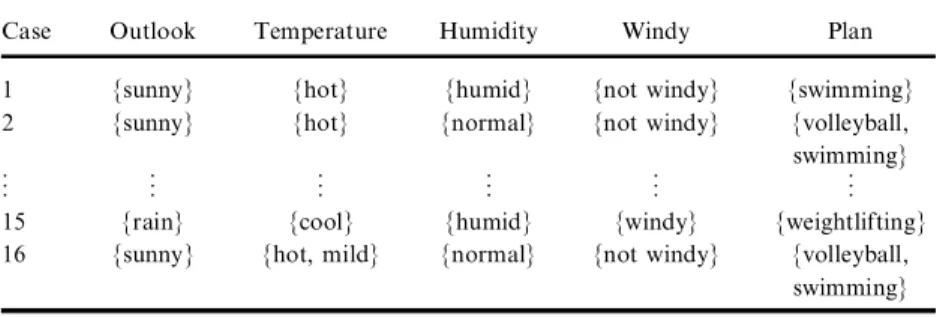
Example 3.1: Under the signi¢cance level a ˆ 0.5, one can translate Table 1 into Table 2 as shown.
The translated fuzzy relation shown in Table 2 can be further reduced into a reduced fuzzy relation such that each attribute’s value of the cases contains the set of linguistic terms whose membership values in Table 2 are larger than the signi¢cance level a ˆ 0.5. In this case, Table 2 can be translated into a reduced fuzzy relation as shown in Table 3. From Table 1, one can see that ``outlook,’’ ``temperature,’’ ``humidity,’’ and ``wind’’ are the attributes of the fuzzy relation, whose values are the sets of linguistic terms {sunny, cloudy, rain}, {hot, mild, cool}, {humid, normal}, {windy, not windy}, respectively; ``plan’’ is called the classi¢cation attribute whose values are ``volleyball,’’ ``swimming,’’ and ``weightlifting,’’ where ``volleyball,’’ ``swimming,’’ and ``weightlifting’’ are called class terms.
De® nition 3.2: Let A be an attribute, and C be the classi¢cation attribute of an instance, and let Ai be a linguistic term of A and Ck
be a class term of C. The degree of correctness of the classi¢cation (Jeng & Liang, 1993), denoted by cc(Ai; Ck), is the ratio of the number of
instances in the decision nodes of the decision trees which have ``A is Ai and C is Ck’’ to the number of instances which have ``A is Ak’’ in
T ab le 1. A fu zz y re la ti on C as e O ut lo ok T em pe ra tu re H um id it y W in d Pl an su nn y cl ou dy ra in ho t m ild co ol hu m id no rm al w in dy no t w in dy vo lle yb al l sw im m in g w ei gh tl if ti ng 1 0. 9 0. 1 0. 0 1. 0 0. 0 0. 0 0. 8 0. 2 0. 4 0. 6 0. 0 0. 8 0. 2 2 0. 8 0. 2 0. 0 0. 6 0. 4 0. 0 0. 0 1. 0 0. 0 1. 0 1. 0 0. 7 0. 0 . . . . . . . . . . . . . . . . . . . . . . . . . . . . . . . . . . . . . . . . . . 15 0. 0 0. 0 1. 0 0. 0 0. 0 1. 0 1. 0 0. 0 0. 8 0. 2 0. 0 0. 0 1. 0 16 1. 0 0. 0 0. 0 0. 5 0. 5 0. 0 0. 0 1. 0 0. 0 1. 0 0. 8 0. 6 0. 0 T ab le 2. A tr an sl at ed fu zz y re la ti on un de r th e si gn i¢ ca nc e le ve la ˆ 0. 5 C as e O ut lo ok T em pe ra tu re H um id it y W in d Pl an su nn y cl ou dy ra in ho t m ild co ol hu m id no rm al w in dy no t w in dy vo lle yb al l sw im m in g w ei gh tl if ti ng 1 0. 9 0. 0 0. 0 1. 0 0. 0 0. 0 0. 8 0. 0 0. 0 0. 6 0. 0 0. 8 0. 0 2 0. 8 0. 0 0. 0 0. 6 0. 0 0. 0 0. 0 1. 0 0. 0 1. 0 1. 0 0. 7 0. 0 . . . . . . . . . . . . . . . . . . . . . . . . . . . . . . . . . . . . . . . . . . 15 0. 0 0. 0 1. 0 0. 0 0. 0 1. 0 1. 0 0. 0 0. 8 0. 0 0. 0 0. 0 1. 0 16 1. 0 0. 0 0. 0 0. 5 0. 5 0. 0 0. 0 1. 0 0. 0 1. 0 0. 8 0. 6 0. 0 768
the decision node of the decision trees. The degree of correctness of the classi¢cation is a real value between zero and one.
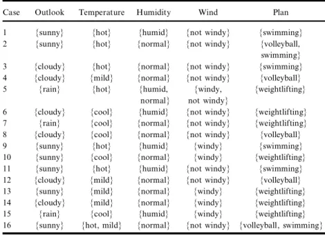
Example 3.2: Based on De¢nition 3.2 one can calculate the degree of correctness of the classi¢cation for each linguistic term in Table 4 shown as follows: cc(sunny; volleyball) ˆ 2/2 ˆ 1, cc(sunny; weightlifting) ˆ 0/2 = 0, cc(cloudy; volleyball) ˆ 3/4 ˆ 0.75, cc(cloudy; weightlifting) ˆ 1/4 ˆ 0.25, cc(hot; volleyball) ˆ 2/2 ˆ 1, cc(hot; weightlifting) ˆ 0, cc(cool; volleyball) ˆ 1/2 ˆ 0.5, cc(cool; weightlifting) ˆ 0.5, cc(mild; volleyball) ˆ 3/3 ˆ 1, cc(mild; weightlifting) ˆ 0/3 ˆ 0, cc(humid; volleyball) ˆ 0/1 ˆ 0, cc(humid; weightlifting) ˆ 1/1 ˆ 1,
Table 3. A reduced fuzzy relation under the signi¢cance level a ˆ 0.5
Case Outlook Temperature Humidity Windy Plan 1 {sunny} {hot} {humid} {not windy} {swimming} 2 {sunny} {hot} {normal} {not windy} {volleyball, swimming} .. . .. . .. . .. . .. . .. . 15 {rain} {cool} {humid} {windy} {weightlifting} 16 {sunny} {hot, mild} {normal} {not windy} {volleyball,
swimming}
Table 4. A reduced fuzzy relation
Case Outlook Temperature Humidity Windy Plan 1 {sunny} {hot} {normal} {not windy} {volleyball} 2 {cloudy} {mild} {normal} {not windy} {volleyball} 3 {cloudy} {cool} {humid} {not windy} {weightlifting} 4 {cloudy} {cool} {normal} {not windy} {volleyball} 5 {cloudy} {mild} {normal} {not windy} {volleyball} 6 {sunny} {hot, mild} {normal} {not windy} {volleyball}
cc(normal; volleyball) ˆ 5/5 ˆ 1, cc(normal; weightlifting) ˆ 0/5 ˆ 0, cc(not windy; volleyball) ˆ 5/6 ˆ 0.833, cc(not windy; weightlifting) ˆ 1/6 ˆ 0.167.
Let C be a classi¢cation attribute with class term C1, C2; . . . ; Ckand
let A be an attribute having m linguistic terms A1, A2; . . . ; Am. The
entropy of A is calculated as follows (Sun, 1995) …1=m† m iˆ1 k jˆ1 ¡pij log pij¡ nijlog nij ; …3† where (1) i ˆ 1, 2, . . . , m and j ˆ 1, 2, . . . , k, (2) pijˆ cc(Ai; Cj), (3) nijˆ 1 ¡ pij.
Example 3.3: According to formula (3) and Table 4, one can calculate the entropy of the attributes ``outlook,’’ ``temperature,’’ ``humidity,’’ and ``wind,’’ respectively, shown as follows:
Entropy of ``outlook’’ ˆ 0.122, Entropy of ``temperature’’ ˆ 0.100,
Entropy of ``humidity’’ ˆ 0, (4)
Entropy of ``wind’’ ˆ 0.196.
In the following, the concept of ``disadvantageous linguistic terms’’ is presented, which will be used in the proposed method for fuzzy classi-¢cation rules generation.
De® nition 3.3: Let b be a disadvantageous threshold value determined by the user, where b2[0,1], Aibe a linguistic term of attribute A, and let
C be the classi¢cation attribute and Cj be a class term of C. If cc(Ai;
Cj) is less than 1-b, we say that Ai is a disadvantageous linguistic term
to Cj.
770 S.-M. CHEN AND S.-Y. LIN
Example 3.4: Assume that the disadvantageous threshold value given by the user is 0.8. Then, based on Example 3.2, we can see that
cc(sunny; weightlifting) < (1¡0.8) = 0.2, cc(hot; weightlifting) < (1¡0.8) ˆ 0.2,
cc(mild; weightlifting) < (1¡0.8) ˆ 0.2, (5)
cc(humid; volleyball) < (1¡0.8) ˆ 0.2.
Thus, one can see that {sunny, hot, mild} and {humid} are disad-vantageous linguistic terms with respect to ``weightlifting’’ and ``volleyball,’’ respectively.
To generate fuzzy classi¢cation rules for forecasting unknown values, one only considers linguistic terms and class terms of an attribute and the classi¢cation attribute, respectively, whose membership values are not less than the signi¢cance level a, a2[0,1], where the value of a is determined by the user. The linguistic terms and the class terms whose membership values are not less than the signi¢cance level a will be kept in the instance of the training data set. For example, if the signi¢cance level a is 0.5, then we can reduce the training data set shown in Table 1 into Table 3.
In the following, a method for generating fuzzy classi¢cation rules is presented from constructed fuzzy decision trees using compound analy-sis techniques. Let a be a signi¢cance level, b be a disadvantageous threshold value, g be a candidate threshold value, and y be a criteria threshold value. The values of a, b, g, and y are given by the user, where a2[0,1], b2[0,1], g2[0,1], y2[0,1], and g µ y. The algorithm for con-structing fuzzy decision trees is presented as follows.
Step 1: Let T contain the training instances which have been reduced by signi¢cance level a, where the linguistic terms and the class terms whose membership value are not less than signi¢cance level a will be kept in the instances of the training data set. Let T be the root node.
Step 2: In T, based on the disadvantageous threshold value b, ¢nd all possible disadvantageous linguistic terms with respect to each class term.
Let D be an empty set. D will record any linguistic term having the degree of correctness of the classi¢cation not less than y
Step 3: Let X, Y, . . . , Z be linguistic terms, S be a set, and Cx,
Cy, . . . , Czbe class terms of the classi¢cation attribute C. Assume there
exists X, Y, . . . , Z in T such that cc(X; Cx)¶cc(Y; Cy)¶ . . . ¶cc(Z; Cz)¶g and S ˆ {X, Y, . . . , Z}.
Step 4: If S is empty, then go to Step 6. Otherwise, go to Step 5. Step 5: Let AKdenote the attribute of linguistic term K. Select a
linguis-tic term K from the set S in the order of X, Y, . . . , Z and remove K from the set S.
If cc(K; Ck)¶y, then create an edge labeled ``Akˆ K’’ from the root
node T to a node labeled Ckas shown in Figure 2 and record any
linguis-tic term d in Ckif d is a disadvantageous linguistic term to class term C.
Put K into the set D. Remove class term Ckof the classi¢cation attribute
C from the instances in T whose attribute Akcontains linguistic term K.
Delete the instances in T whose classi¢cation attribute is empty. If S is empty, then go to Step 2
else go to Step 5
else if S is empty go to Step 2. else go to Step 5.
Step 6: If T is empty, then stop. Otherwise, let A be an attribute in node T having linguistic terms A1, A2, . . . , Am, where A has the minimum
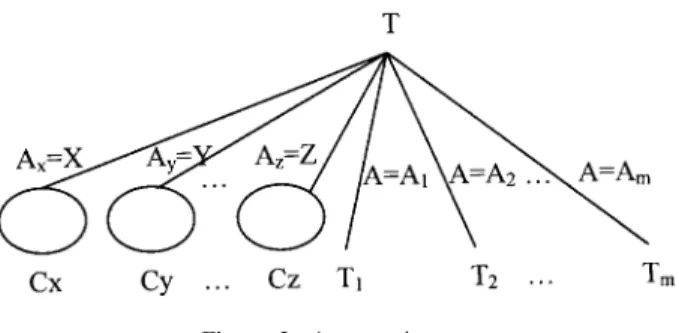
``entropy’’ using formula (3). Sprout the tree from the node T as shown
Figure 2. A sprouting tree.
772 S.-M. CHEN AND S.-Y. LIN
in Figure 2 and let each Ti be a new T, where node Ti contains the
instances whose attribute A contains the linguistic term Aiand 1 µ i µ m.
Go to Step 2.
Figure 3 shows an example of a fuzzy decision tree, where we assume that X is a disadvantageous linguistic term to C2 denoted by X
C2
®, X and
Y are disadvantageous linguistic terms to C3 denoted by , X
and Z are disadvantageous linguistic terms to C2 denoted by
and Y and Z are disadvantageous linguistic terms to C1 denoted by
. From the constructed fuzzy decision tree shown in Figure 3, one can generate the fuzzy classi¢cation rules shown in Table 5 from the root node to the leaf nodes of the fuzzy decision tree, where X, Y, Z, E, and F are linguistic terms of the attributes Ax, Ay, Az, Ae, and Af, respectively,
Figure 3. An example of the constructed fuzzy decision.
Table 5. Generated fuzzy classi¢cation rules
Rule 1: IF Axis X THEN C is C1
Rule 2: IF Ayis Y and Axis X THEN C is C2
.. .
Rule k: IF Azis Z and Axis X and Ay is Y THEN C is C3
Rule k ‡ 1: IF A is A1and Aeis E and Axis X and Ayis Y THEN C is C3
Rule k ‡ 2: IF A is A1and Afis F and Axis X and Azis Z THEN C is C2
Rule k ‡ 3: IF A is A2 and Axis X and Azis Z THEN C is C2
.. .
Rule n: IF A is Amand Ayis Y and Azis Z THEN C is C1
T ab le 6. A sm al l tr ai ni ng da ta se t (Y ua n et al ., 19 95 ) O ut lo ok T em pe ra tu re H um id it y W in d Pl an C as e su nn y cl ou dy ra in ho t m ild co ol hu m id no rm al w in dy no t w in dy vo lle yb al l sw im m in g w ei gh tl if ti ng 1 0. 9 0. 1 0. 0 1. 0 0. 0 0. 0 0. 8 0. 2 0. 4 0. 6 0. 0 0. 8 0. 2 2 0. 8 0. 2 0. 0 0. 6 0. 4 0. 0 0. 0 1. 0 0. 0 1. 0 1. 0 0. 7 0. 0 3 0. 0 0. 7 0. 3 0. 8 0. 2 0. 0 0. 1 0. 9 0. 2 0. 8 0. 3 0. 6 0. 1 4 0. 2 0. 7 0. 1 0. 3 0. 7 0. 0 0. 2 0. 8 0. 3 0. 7 0. 9 0. 1 0. 0 5 0. 0 0. 1 0. 9 0. 7 0. 3 0. 0 0. 5 0. 5 0. 5 0. 5 0. 0 0. 0 1. 0 6 0. 0 0. 7 0. 3 0. 0 0. 3 0. 7 0. 7 0. 3 0. 4 0. 6 0. 2 0. 0 0. 8 7 0. 0 0. 3 0. 7 0. 0 0. 0 1. 0 0. 0 1. 0 0. 1 0. 9 0. 0 0. 0 1. 0 8 0. 0 1. 0 0. 0 0. 0 0. 2 0. 8 0. 2 0. 8 0. 0 1. 0 0. 7 0. 0 0. 3 9 1. 0 0. 0 0. 0 1. 0 0. 0 0. 0 0. 6 0. 4 0. 7 0. 3 0. 2 0. 8 0. 0 10 0. 9 0. 1 0. 0 0. 0 0. 3 0. 7 0. 0 1. 0 0. 9 0. 1 0. 0 0. 3 0. 7 11 0. 7 0. 3 0. 0 1. 0 0. 0 0. 0 1. 0 0. 0 0. 2 0. 8 0. 4 0. 7 0. 0 12 0. 2 0. 6 0. 2 0. 0 1. 0 0. 0 0. 3 0. 7 0. 3 0. 7 0. 7 0. 2 0. 1 13 0. 9 0. 1 0. 0 0. 2 0. 8 0. 0 0. 1 0. 9 1. 0 0. 0 0. 0 0. 0 1. 0 14 0. 0 0. 9 0. 1 0. 0 0. 9 0. 1 0. 1 0. 9 0. 7 0. 3 0. 0 0. 0 1. 0 15 0. 0 0. 0 1. 0 0. 0 0. 0 1. 0 1. 0 0. 0 0. 8 0. 2 0. 0 0. 0 1. 0 16 1. 0 0. 0 0. 0 0. 5 0. 5 0. 0 0. 0 1. 0 0. 0 1. 0 0. 8 0. 6 0. 0 774
and C1, C2, and C3are class terms of the classi¢cation attribute C, where
``X’’ means the complement of X (i.e., not X).
Example 3.5: Assume that the signi¢cance level a given by the user is 0.5, using the training data set presented in Yuan and Shaw (1995) as shown in Table 6. By Step 1 of the proposed algorithm, one can reduce Table 6 into Table 7 under the signi¢cance level a ˆ 0.5, where ``plan’’ is the classi¢cation attribute and ``volleyball,’’ ``swimming,’’ and ``weightlifting’’ are the class terms of the classi¢cation attribute ``plan.’’ Assume that the disadvantageous threshold value b ˆ 0.8, the can-didate threshold value g ˆ 0.8, and the criteria threshold value y ˆ 1.0; then, initially, the root node contains the instances of the reduced train-ing data set under the signi¢cance level a ˆ 0.5 as shown in Table 7. (i) First iteration: Based on Step 2 of the proposed algorithm, we can see
that
Table 7. Reduced training data set under the signi¢cance level a ˆ 0.5
Case Outlook Temperature Humidity Wind Plan 1 {sunny} {hot} {humid} {not windy} {swimming} 2 {sunny} {hot} {normal} {not windy} {volleyball,
swimming} 3 {cloudy} {hot} {normal} {not windy} {swimming} 4 {cloudy} {mild} {normal} {not windy} {volleyball} 5 {rain} {hot} {humid, {windy, {weightlifting}
normal} not windy}
6 {cloudy} {cool} {humid} {not windy} {weightlifting} 7 {rain} {cool} {normal} {not windy} {weightlifting} 8 {cloudy} {cool} {normal} {not windy} {volleyball} 9 {sunny} {hot} {humid} {windy} {swimming} 10 {sunny} {cool} {normal} {windy} {weightlifting} 11 {sunny} {hot} {humid} {not windy} {swimming} 12 {cloudy} {mild} {normal} {not windy} {volleyball} 13 {sunny} {mild} {normal} {windy} {weightlifting} 14 {cloudy} {mild} {normal} {windy} {weightlifting} 15 {rain} {cool} {humid} {windy} {weightlifting} 16 {sunny} {hot, mild} {normal} {not windy} {volleyball, swimming}
{rain, humid, windy} are disadvantageous linguistic terms to the class term ``volleyball’’;
{rain, cool} are disadvantageous linguistic terms to the class term ``swimming’’;
{hot} is a disadvantageous linguistic term to the class term ``weightlifting’’.
Based on Step 3 of the proposed algorithm, one can get the set S of linguistic terms to produce classi¢cations under the candidate threshold value g ˆ 0.8, where
S ˆ {rain, hot, windy, cool}.
Since ``rain,’’ ``hot,’’ and ``windy’’ can produce classi¢cations (i.e., they have the degrees of correctness of the classi¢cation not less than the criteria threshold value y, where y ˆ 1.0) after applying Step 4, and Step 5 of the proposed algorithm one can partially construct the fuzzy decision tree shown in Figure 4, where the linguistic terms printed in the leaf nodes of the partially constructed fuzzy decision tree are the disadvantageous linguistic terms to the corresponding class term, i.e., ``rain’’ is a disadvantageous linguistic term with respect to the class term ``swimming’’; ``hot’’ is a disadvantageous linguistic term with respect to the class term ``weightlifting.’’
(ii) Second iteration: After applying the second iteration of the proposed algorithm (i.e., Step 2, Step 3, Step 4, Step 5, and Step 6), we have S ˆ {humid, normal, sunny, hot, mild, not windy}. In this case,
Figure 4. Partially constructed fuzzy decision tree.
776 S.-M. CHEN AND S.-Y. LIN
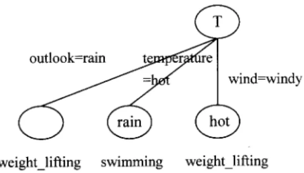
``humid’’ and ``normal’’ produce classi¢cations (i.e., they have the degree of correctness of the classi¢cation not less than the criteria threshold value y, where y ˆ 1.0). The ¢nal constructed fuzzy decision tree is shown in Figure 5, where the linguistic terms printed in the leaf nodes of the constructed fuzzy decision tree are the disadvantageous linguistic terms to the corresponding class term.
Based on the constructed fuzzy decision tree shown in Figure 5, we can get the fuzzy classi¢cation rules shown as follows:
Rule 1: IF outlook is rain THEN plan is weightlifting.
Rule 2: IF temperature is hot AND outlook is rain THEN plan is
swimming.
Rule 3: IF wind is windy AND temperature is hot THEN plan is
weightlifting.
Rule 4: IF humidity is humid AND temperature is hot THEN plan is
weightlifting.
Rule 5: IF humidity is normal AND outlook is rain AND wind is windy THEN plan is volleyball.
where rain is the complement of rain (i.e., NOT Rain), windy is the comp-lement of windy (i.e., NOT windy), and hot is the compcomp-lement of hot (i.e., NOT hot), respectively.
One can apply the generated fuzzy classi¢cation rules to deal with the classi¢cation problems. A fuzzy classi¢cation rule has the following form:
Figure 5. A constructed fuzzy decision tree.
IF A is Ai AND B is Bj THEN C is Ck,
where A and B are attributes of an instance, Ai and Bj are linguistic
terms of A and B, respectively; Ckis a class term of the classi¢cation
attribute C. Then, one can forecast the value of the term Ckof the
classi-¢cation attribute C. Let a and b be the membership values of the instance in Ai and Bj, respectively. Let c be the forecasted value of Ck, where
c ˆ min(a, b). When two or more fuzzy classi¢cation rules have the same conclusion (i.e., they all conclude that ``IF conditions THEN C is Ck’’),
then one generates several forecasted values with respect to Ck, and
one takes the largest one.
Based on the generated fuzzy classi¢cation rules described above, one can use them to get the forecasted membership values of each class term of the classi¢cation attribute. For example, by applying the above ¢ve fuzzy classi¢cation rules to case 1 shown in Table 6, we can get the forecasted membership values for case 1 with respect to the class terms ``volleyball,’’ ``swimming,’’ and ``weightlifting,’’ respectively, shown as follows:
(1) Based on Rule 5 and Table 6, we can see that
(i) The degree of membership of ``humidity is normal’’ for case 1 is 0.2.
(ii) The degree of membership of ``outlook is rain’’ for case 1 is 0.0. Thus, the degree of membership of ``outlook is rain’’ for case 1 is equal to 1.0¡0.0 ˆ 1.0.
(iii) The degree of membership of ``wind is windy’’ for case 1 is 0.4. Thus, the degree of membership of ``outlook is windy’’ for case 1 is equal to 1.0¡0.4 ˆ 0.6.
Thus, the forecasted membership value for case 1 with respect to the class term ``volleyball’’ can be evaluated as follows: min(0.2, 1.0¡0.0, 1.0¡0.4)
ˆ min (0.2, 1.0, 0.6) ˆ 0.2.
(2) Based on Rule 2 and Table 6, one can see that
778 S.-M. CHEN AND S.-Y. LIN
(i) The degree of membership of ``temperature is hot’’ for case 1 is 1.0.
(ii) The degree of membership of ``outlook is rain’’ for case 1 is 0.0. Thus, the degree of membership of ``outlook is rain’’ for case 1 is equal to 1.0¡0.0 ˆ 1.0.
Thus, the forecasted membership value for case 1 with respect to the class term ``swimming’’ can be evaluated as follows: min(1.0, 1.0¡0.0)
ˆ min (1.0, 1.0) ˆ 1.0.
(3) (a) Based on Rule 1 and Table 6, one can see that the degree of mem-bership of ``outlook is rain’’ for case 1 is 0.0.
(b) Based on Rule 3 and Table 6, we can see that
(i) The degree of membership of ``wind is windy’’ for case 1 is 0.4.
(ii) The degree of membership of ``temperature is hot’’ of case 1 is 1.0. Thus, the degree of membership of ``temperature is
hot ’’ for case 1 is equal to 1.0¡1.0 ˆ 0.0.
(c) Based on Rule 4 and Table 6, one can see that
(i) The degree of membership of ``humidity is humid’’ for case 1 is 0.8.
(ii) The degree of membership of ``temperature is hot’’ for case 1 is 1.0. Thus, the degree of membership of ``temperature is hot ’’ for case 1 is equal to 1.0¡1.0 ˆ 0.0.
From (a), (b), and (c), the forecasted membership value for case 1 with respect to the class term ``weightlifting’’ can be evaluated as follows:
max[0.0, min (0.4, 1.0¡1.0), min(0.8, 1.0¡1.0)] ˆ max [0.0, min(0.4, 0.0), min (0.8, 0.0)] ˆ max [0.0, 0.0, 0.0]
ˆ 0.0.
Similarly, one can get the forecasted membership values of ``volleyball,’’ ``swimming,’’ and ``weightlifting’’ through Case 2 to Case 16 shown as follows:
Case 2: volleyball ˆ 1.0, swimming ˆ 0.6, weightlifting ˆ 0.0, Case 3: volleyball ˆ 0.7, swimming ˆ 0.7, weightlifting ˆ 0.3, Case 4: volleyball ˆ 0.7, swimming ˆ 0.3, weightlifting ˆ 0.3, Case 5: volleyball ˆ 0.1, swimming ˆ 0.1, weightlifting ˆ 0.9, Case 6: volleyball ˆ 0.3, swimming ˆ 0.0, weightlifting ˆ 0.7, Case 7: volleyball ˆ 0.3, swimming ˆ 0.0, weightlifting ˆ 0.7, Case 8: volleyball ˆ 0.8, swimming ˆ 0.0, weightlifting ˆ 0.2, Case 9: volleyball ˆ 0.3, swimming ˆ 1.0, weightlifting ˆ 0.0, Case 10: volleyball ˆ 0.1, swimming ˆ 0.0, weightlifting ˆ 0.9, Case 11: volleyball ˆ 0.0, swimming ˆ 1.0, weightlifting ˆ 0.0, Case 12: volleyball ˆ 0.7, swimming ˆ 0.0, weightlifting ˆ 0.3, Case 13: volleyball ˆ 0.0, swimming ˆ 0.2, weightlifting ˆ 0.8, Case 14: volleyball ˆ 0.3, swimming ˆ 0.0, weightlifting ˆ 0.7, Case 15: volleyball ˆ 0.0, swimming ˆ 0.0, weightlifting ˆ 1.0, Case 16: volleyball ˆ 1.0, swimming ˆ 0.5, weightlifting ˆ 0.0. In the next section, experimental results of the proposed method will be compared with that of Yuan and Shaw’s method (1995) by assigning the parameters of the signi¢cance level a, the disadvantageous threshold value b, the candidate threshold value g, and the criteria threshold value y to construct fuzzy decision trees and generate fuzzy classi¢cation rules, where a2[0,1], b2[0,1], g2[0,1], y2[0,1], and g µ y. The Turbo C version 3.0 has been used on a PC/AT to implement the proposed algorithm for constructing fuzzy classi¢cation trees and generating fuzzy classi¢-cation rules. By using the generated fuzzy classi¢classi¢-cation rules, one can forecast the membership values of the class terms of the classi¢cation attributes.
EXPERIM ENT ANALYSIS
In the following, it will be assumed that the signi¢cance level a ˆ 0.5, the disadvantageous threshold value b ˆ 0.8, the candidate threshold value g ˆ 0.8, and the criteria threshold value y ˆ 1.0. Comparative results between the proposed method and Yuan and Shaw’s method (1995) con-cerning the number of edges in the constructed fuzzy decision tree, the number of decision nodes involving the computations of the entropy of the attributes, and the classi¢cation accuracy rate will also be dis-cussed.
780 S.-M. CHEN AND S.-Y. LIN
Yuan and Shaw (1995) used the data shown in Table 6 to generate six fuzzy classi¢cation rules shown below under the signi¢cance level ˆ 0.5 and the truth level ˆ 0.7. It is obvious that Yuan and Shaw’s method generated more fuzzy classi¢cation rules than the proposed method. One can see that the proposed method only generated ¢ve fuzzy decision rules, while Yuan and Shaw’s method generated six fuzzy classi-¢cation rules. In the following, the classiclassi-¢cation results of Yuan and Shaw’s method (1995) and the classi¢cation results of the proposed method are compared as shown in Table 8 and Table 9. As mentioned in Yuan and Shaw (1995), the classi¢cation accuracy rate is the ratio of the number of instances (cases) in the training data set, which are cor-rectly classi¢ed to the number of total instances in the training data set. As described above, one can see that the classi¢cation accuracy rate of the proposed method is 0.9375, while the classi¢cation accuracy rate of Yuan and Shaw’s method is 0.8125.
The comparison between Yuan and Shaw’s method and the pro-posed method concerning the number of edges in the constructed fuzzy decision tree, the number of decision nodes in the fuzzy decision trees that involve the computations of the entropy of the attribute, and the classi¢cation accuracy rate are shown in Table 10.
From Table 10, one can see that Yuan and Shaw’s method has the classi¢cation accuracy rate equal to 0.8125 (under the parameters that the signi¢cance level is 0.5 and the truth level threshold is 0.7), while the proposed method has the classi¢cation accuracy rate equal to 0.9375 (under the signi¢cance level a ˆ 0.5, the disadvantageous threshold value b ˆ 0.8, the candidate threshold value g ˆ 0.8, and the criteria threshold value y ˆ 1.0). Furthermore, one also can see that the proposed method generates less edges and decision nodes in the constructed fuzzy decision tree than the one presented in (Yuan and Shaw, 1995).
CONCLUSIONS
In this article, a new method has been presented for constructing fuzzy decision tree and generating fuzzy classi¢cation rules from the con-structed fuzzy decision trees, using the compound analysis techniques. An experiment has also been made to compare the proposed method with Yuan and Shaw’s method (1995). From the experimental results, one can see that the proposed method has the following advantages:
Table 8. Compare Yuan and Shaw’s classi¢cation results with known classi¢cation results
Classi¢cation Known in Training Data (Yuan et al., 1995) (see Table 6) Plan
Case Volleyball Swimming Weightlifting
1 0.0 0.8 0.2 2 1.0 0.7 0.0 3 0.3 0.6 0.1 4 0.9 0.1 0.0 5 0.0 0.0 1.0 6 0.2 0.0 0.8 7 0.0 0.0 1.0 8 0.7 0.0 0.3 9 0.2 0.8 0.0 10 0.0 0.3 0.7 11 0.4 0.7 0.0 12 0.7 0.2 0.1 13 0.0 0.0 1.0 14 0.0 0.0 1.0 15 0.0 0.0 1.0 16 0.8 0.6 0.0
Classi¢cation Results with Learned Rules by Yuan and Shaw’s Method (Yuan et al., 1995)
Plan
Case Volleyball Swimming Weightlifting
1 0.0 0.9 0.0 2 0.4 0.6 0.0 (#) 3 0.2 0.7 0.3 4 0.7 0.3 0.3 5 0.3 0.1 0.9 6 0.3 0.0 0.7 7 0.0 0.0 1.0 8 0.2 0.0 0.8 (#) 9 0.0 1.0 0.0 10 0.1 0.0 0.7 11 0.0 0.7 0.0 12 0.7 0.0 0.3 13 0.0 0.2 0.8 14 0.3 0.0 0.7 15 0.0 0.0 1.0 16 0.5 0.5 0.0 (*)
(#) Wrong classi¢cation; (*) Cannot distinguish between two or more classes.
782 S.-M. CHEN AND S.-Y. LIN
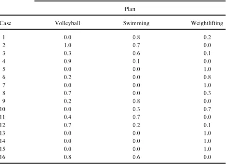
Table 9. Compare our classi¢cation results with known classi¢cation results
Classi¢cation Known in Training Data (Yuan et al., 1995) (see Table 6) Plan
Case Volleyball Swimming Weightlifting
1 0.0 0.8 0.2 2 1.0 0.7 0.0 3 0.3 0.6 0.1 4 0.9 0.1 0.0 5 0.0 0.0 1.0 6 0.2 0.0 0.8 7 0.0 0.0 1.0 8 0.7 0.0 0.3 9 0.2 0.8 0.0 10 0.0 0.3 0.7 11 0.4 0.7 0.0 12 0.7 0.2 0.1 13 0.0 0.0 1.0 14 0.0 0.0 1.0 15 0.0 0.0 1.0 16 0.8 0.6 0.0
Classi¢cation Results with Learned Rules by the Proposed Method Plan
Case Volleyball Swimming Weightlifting
1 0.2 1.0 0.0 2 1.0 0.6 0.0 3 0.7 0.7 0.3 (*) 4 0.7 0.3 0.3 5 0.1 0.1 0.9 6 0.3 0.0 0.7 7 0.3 0.0 0.7 8 0.8 0.0 0.2 9 0.3 1.0 0.0 10 0.1 0.0 0.9 11 0.0 1.0 0.0 12 0.7 0.0 0.3 13 0.0 0.2 0.8 14 0.3 0.0 0.7 15 0.0 0.0 1.0 16 1.0 0.5 0.0
(*) Cannot distinguish between two or more classes.
(1) The proposed method could get a better classi¢cation accuracy rate than the one presented in Yuan and Shaw (1995). From Table 10, one can see that the classi¢cation accuracy rate of the proposed method is 0.9375, and the classi¢cation rate of Yuan and Shaw’s method is 0.8125. Furthermore, the proposed method generates less branch edges and decision nodes than the one presented in Yuan and Shaw (1995).
(2) The proposed method generated less fuzzy classi¢cation rules. From the illustrated example, one can see that the proposed method gen-erated ¢ve fuzzy classi¢cation rules but Yuan and Shaw’s method generated six fuzzy classi¢cation rules.
REFERENCES
Boyen, X., and L. Wehenkel. 1999. Automatic induction of fuzzy decision trees and its application to power system security assessment. Fuzzy Sets Syst. 102(1):3^19.
Chang, R. L. P., and T. Pavlidis. 1977. Fuzzy decision tree algorithms. IEEE
Trans. Syst., Man, Cybern 7(1):28^35.
Chen, S. M. 1988. A new approach to handling fuzzy decision making problems.
IEEE Trans. Syst., Man, Cybern. 18(6):1012^1016.
Chen, S. M., and M. S. Yeh. 1997. Generating fuzzy rules from relational database systems for estimating null values. Cybernetics and Systems: An
International Journal 28(8):695^723.
Hart, A. 1995. The role of induction in knowledge elicitation, Expert Systems 2(1):24^28.
Hunt, E. B., J. Marin, and P. J. Stone. 1966. Experience in induction. New York: Academic Press.
Jeng, B., and T. P. Liang. 1993. Fuzzy indexing and retrieval in case-based systems. In Proc. 1993 Pan Paci¢c Conference on Information Systems, Taiwan, R. O. C., 258^266.
Table 10. Comparison between Yuan and Shaw’s method and the proposed method
Yuan and Shaw’s The Proposed Method (Yuan et al., 1995) Method
Number of branch edges 8 5
Number of decision nodes 3 2
Classi¢cation accuracy rate 0.8125 0.9375
784 S.-M. CHEN AND S.-Y. LIN
Lin, S. Y., and S. M. Chen. 1996. A new method for generating fuzzy rules from fuzzy decision trees. In Proc. 7th International Conference on Information
Management, Chungli, Taoyuan, Taiwan, R. O. C., 358^364.
Mingers, J. 1989. An empirical comparison of pruning methods for decision tree induction. Machine Learning 4(2):227^243.
Quinlan, J. R. 1979. Discovering rules by induction from large collection of examples. In Expert systems in the micro electronic age, D. Michie, ed. Edinburgh: Edinburgh University Press.
Quinlan, J. R. 1986. Introduction of decision trees. Machine Learning 1(1):81^106.
Quinlan, J. R. 1990. Decision trees and decisionmaking. IEEE Trans. Syst., Man,
Cybern. 20(2):339^346.
Safavian, S. R., and D. Landgrebe. 1991. A survey of decision tree classi¢er methodology. IEEE Trans. Syst., Man, Cybern. 21(3):660^674.
Sun, S. W. 1995. A fuzzy approach to decision trees. M.S. Thesis, Institute of Computer and Information Science, National Chiao Tung University, Hsinchu, Taiwan, R. O. C.
Wu, T. P., and S. M. Chen. 1999. A new method for constructing membership functions and fuzzy rules from training examples. IEEE Trans. Syst., Man,
Cybern.öPart B 29(1):25^40.
Yasdi, R. 1991. Learning classi¢cation rules from database in the context of knowledge acquisition and representation. IEEE Trans. Syst., Man, Cybern. 3(3):293^306.
Yeh, M. S., and S. M. Chen. 1995. An algorithm for generating fuzzy rules from relational database systems. In Proc. 6th International Conference on
Infor-mation Management, Taipei, Taiwan, R. O. C., 219^226.
Yuan, Y., and M. J. Shaw. 1995. Induction of fuzzy decision trees. Fuzzy Sets
Syst. 69(2):125^139.
Zadeh, L. A. 1965. Fuzzy sets. Inf. Contr. 8:338^353.
Zadeh, L. A. 1975. The concepts of a linguistic variable and its application to approximate reasoning (I). Information Sciences 8:199^249.