Trihalomethane Species Forecast Using Optimization
Methods: Genetic Algorithms and Simulated Annealing
Yu-Chung Lin
1and Hund-Der Yeh
2Abstract:Chlorination is an effective method for disinfection of drinking water. Yet chlorine is a strong oxidizing agent and easily reacts
with both organic and inorganic materials. Trihalomethanes共THMs兲, formed as a by-product of chlorination, are carcinogenic to humans.
Models can be derived from linear and nonlinear multiregression analyses to predict the THM species concentration of empirical reaction kinetic equations. The main objective of this study is to predict the concentrations of THM species by minimizing the nonlinear function,
representing the errors between the measured and calculated THM concentrations, using the genetic algorithm 共GA兲 and simulated
annealing 共SA兲. Additionally, two modifications of SA are employed. The solutions obtained from GA and SA are compared with the
measured values and those obtained from a generalized reduced gradient method共GRG2兲. The results indicate that the proposed heuristic
methods are capable of optimizing the nonlinear problem. The predicted concentrations may provide useful information for controlling the chlorination dosage necessary to assure the safety of water drinking.
DOI:10.1061/共ASCE兲0887-3801共2005兲19:3共248兲
CE Database subject headings: Algorithms; Evolutionary computation; Simulation; Disinfection; Optimization; Chlorination; Potable water.
Introduction
The basic operations in a water treatment plant include three major processes such as clarification, filtration, and disinfection. Removal of pathogenic microorganisms, tastes, odors, color, tur-bidity, dissolved minerals, and harmful organic materials are very important in water treatment. Water contains many microorgan-isms, some of which cause diseases. Typical bacterial reductions of 60 to 70% are possible by coagulation, flocculation, and sedi-mentation. A filtration process increases the overall bacterial re-moval to about 99%. Disinfection is an essential and final barrier against human exposure to disease-causing pathogenic microor-ganisms in water supply engineering.
Chlorination began at the start of the last century to provide an additional safeguard against pathogenic microorganisms. A num-ber of equilibria affect the form and the effectiveness of chlorine in water. Chlorine is a very strong oxidizing agent and may com-bine with water to form hypochlorous and hydrochloric acids 共Bitton 1999兲.
Hypochlorous and hydrochloric acids react with both organic
and inorganic materials to produce trihalomethanes 共THMs兲.
Chloroform 共CHCl3兲, bromodichloromethane 共CHBrCl2兲,
dibromochloromethane 共CHBr2Cl兲, and bromoform 共CHBr3兲,
produced by chlorination of water and wastewater, are suspected mutagens/carcinogens. Because of their carcinogenic effect, the
U.S. Environmental Protection Agency共USEPA兲 limited the
con-centration of four kinds of THM species in recent years. The USEPA finalized the new disinfectant/disinfection by-products rules in 1998 and limited the residual chlorine concentration to 0.08 mg/ L in drinking water. A recent study by the USEPA found that women exposed to higher levels of chlorine by-products had a 15.7% risk of miscarriage, whereas those who had little
expo-sure to THM had a lower共9.5%兲 risk 共Elshorbagy 2000兲.
Elshorbagy 共2000兲 applied a generalized reduced gradient
method 共GRG2兲, developed by Lasdon and Warren 共1982兲, to
characterize and simulate the kinetics of THM species under rep-resentative extreme conditions associated with temperature, chlo-rine dosage, and bromide content. The GRG2 model was em-ployed to combine site-specific trends with stoichiometric expressions based on an average representative bromine concen-tration factor. The model was evaluated, tested, and validated using data from finished desalinated water collected in the United
Arab Emirates. Elshorbagy 共2000兲 obtained reasonable
agree-ments between predicted and measured values of different
spe-cies. Milot et al.共2002兲 applied artificial neural networks to
pre-dict the contaminant levels of total THMs in the chlorinated water under laboratory condition.
The objective of this study was to find the concentrations of THM species by minimizing the nonlinear function representing the errors between the measured and calculated THM
concentra-tions. Results obtained from genetic algorithm 共GA兲 and
simu-lated annealing共SA兲 are compared with the measured values and
those obtained from the GRG2 model. The proposed methods provide a useful tool for controlling the chlorination dosage to assure the safety of water drinking.
1
Graduate Student, Institute of Environment Engineering, National Chiao-Tung Univ., Hsinchu, Taiwan.
2Professor, Institute of Environment Engineering, National Chiao-Tung Univ., Hsinchu, Taiwan.
Note. Discussion open until December 1, 2005. Separate discussions must be submitted for individual papers. To extend the closing date by one month, a written request must be filed with the ASCE Managing Editor. The manuscript for this paper was submitted for review and pos-sible publication on August 22, 2003; approved on December 9, 2004. This paper is part of the Journal of Computing in Civil Engineering, Vol. 19, No. 3, July 1, 2005. ©ASCE, ISSN 0887-3801/2005/3-248–257/ $25.00.
Studies on Trihalomethane Formation
Many researchers discovered that THM formation potential is a
useful and conservative indicative parameter 共Rook 1974; Bunn
et al. 1975; Trussel and Umphres 1978; Minear 1980兲. The
in-dicative parameter could apparently develop in the presence of total available organic precursors. Those studies also showed that THM levels increase with increasing bromide concentration.
Gould et al. 共1981兲 defined the bromine incorporation factor
共BIF兲, which changes little with reaction time. The pH and or-ganic precursor content, depending on the bromide concentration,
have a maximum influence on BIF. Montgomery Watson共1993兲
also found that bromide-rich sources of water such as desalinated and/or some groundwater wells can increase the THM formation potential. Various parameters, such as total organic carbon, ultra-violet light absorbance, temperature, chlorine dosage, bromide concentration, reaction time, and chlorination pH also affect THM formation.
Clark et al. 共1994兲 presented certain dynamic water quality
studies to treat THM as a conservative substance throughout the distribution system and to approximate its kinetics by a first order, growth-limited reaction rate expression. More recently, Clark 共1998兲 proposed an improved model based on second-order reac-tion kinetics for THM formareac-tion as a funcreac-tion of chlorine
de-mand. In contrast, Nokes et al.共1999兲 proposed a reaction scheme
with another kinetic model to simulate the THM formation. The mathematical model related the extent of bromination and the
relative abundances of the four THM species to the关Br−兴:关Cl−兴
ratio.
In addition to the dynamic models mentioned previously, some empirical models were also proposed to describe the mechanisms
of THM formation共e.g., Amy et al. 1987; Adin et al. 1991;
Golfi-nopoulos et al. 1998兲. Among the empirical models, Amy et al.
共1987兲 examined the relationships between several key water quality parameters and their corresponding THM formation. Based on the empirical results, a multiparameter power function, derived from linear and nonlinear multiregression, was developed to predict THM formation in drinking water.
Development and Application of the Heuristic Approaches
Recently, considerable attention has been paid on stochastic opti-mization techniques such as GA and SA. The predominance of these heuristic methods is that the optimization problem is al-lowed to be formulated as a nonlinear or mixed integer problem. The user does not need much experience in providing the initial guesses for solving nonlinear problems. This is the major differ-ence between the heuristic algorithm and the traditional approach such as Newton’s method and/or GRG2. The main advantage of using the heuristic algorithm is that it can solve the problem with arbitrary initial guesses and may give optimal results without any rules. Two heuristic methodologies, GA and SA, will be adopted in this study for the optimal determination of the concentration of THMs.
GA was developed by Holland共1975兲 in the 1950s and 1960s.
Darwin’s theory of evolution is the basic concept of GA. Using a population of guesses in GA to solve the optimization problem significantly differs from those solvers using a single guess. The main idea is that the genetic information of a good solution spreads over the entire population. Thus, the best solution can be obtained by thoroughly combining the “chromosomes” in the population. Selection, crossover, mutation, and reproduction are
the essential operators in GA. The selection operator picks up the relative fitter strings according to their objective function values. Then the newborn trial solutions are generated from the relative fitter string with the crossover operator. Avoiding the trial solution trapped in a local region is the main idea behind the mutation operator.
In recent years, GA has been applied in a variety of fields.
McKinney and Lin共1994兲 presented a groundwater management
model using GA. Lippai et al.共1999兲 performed robust analysis
and optimization of a water distribution network based on GA-based optimizers with Win-Pipes.EXE, a Windows program GA-based on the EPANET source code. They applied this method on the New York City Water Supply Tunnel problem and the results obtained meet the multiple goals of a reliable, low-cost water distribution system, and also satisfy the maximum hour demands
and fire flow demands. Gupta et al.共1999兲 presented a
methodol-ogy for minimizing the cost of a pipe network using GA. The
solution set obtained from GA and nonlinear programming共NLP兲
techniques for several medium size networks showed that GA provided a better solution in general, in comparison with that obtained with NLP techniques. GA is a general stochastic evolu-tionary algorithm with a wide range of applicability to
optimiza-tion problems with good performance 共Coley 1999; Pham and
Karaboga 2000兲. Gwo 共2001兲 used a simple GA to search for
preferential flow in a structured porous media. The result showed that GA can invert the correct pictures of simple fracture net-works.
Another heuristic method employed in this study is SA.
Me-tropolis et al.共1953兲 first applied SA in a two-dimensional
rigid-sphere system. Kirkpatrick et al. 共1983兲 demonstrated the
strengths of SA by solving large-scale combinatorial optimization problems. SA is a random search algorithm that allows, at least in theory or in probability, to obtain the global optimum of a
func-tion in any given domain 共Aarts and Korst 1989兲. One of the
advantages of SA is its ability to use a descent strategy which allows random ascent moves to avoid possible traps in a local optimum. Ease of implementation is another advantage of SA.
Goffe et al. 共1994兲 presented the results of global optimization
stochastic functions with SA. Cunha and Sousa共1999兲 used SA to
minimize the costs of a water distribution network. Pham and
Karaboga共2000兲 demonstrated that SA can be applied for a wide
range of optimization applications. Domer et al. 共2003兲 applied
SA to control the quasi-static displacement of a tensegrity struc-ture with multiple objectives and interdependent actuator effects. Their results suggest that SA provide a rapid convergence to “good” solutions.
These two heuristic approaches could obtain the global opti-mal solutions. However, when the problem or the solution space is fairly complicated, heuristic approaches may have the problems of taking much computing time and effort to solve the optimiza-tion problem. Differing from the gradient type approach, the heu-ristic approaches should generate the trial solutions in the speci-fied solution space. In addition, all the trial solutions require calculating the objective function values even though those
solu-tions are incorrect. Besides, Youssef et al.共2001兲 pointed out that
if excess population size and/or maximum evolutionary genera-tion were specified, GA also took much time and effort to obtain global optimum solutions. Similar to SA, the local optimum so-lution would be obtained if the initial temperature given was too low. On the other hand, if a higher initial temperature was given, more time would be consumed for using SA.
Methodology
In this section, the kinetics of THM and THM species, GA, and SA are described separately. An exhaustive description to simu-late the THM formation and formusimu-late the objective function is given first. The detailed general idea and algorithm of GA and SA are also presented.
Kinetics of Trihalomethane and Trihalomethane Species
THM compounds are commonly developed in chlorinated water containing organic precursors, such as humic and fulvic acids.
Total trihalomethane 共TTHM兲 is known to increase with time;
however, information about the reaction mechanism of THM and its species is still limited.
Trihalomethane Simulation
Let 关THM0兴, 关THM1兴, 关THM2兴, and 关THM3兴 be the molar con-centrations of the four THM species: Chloroform, bromodichlo-romethane, dibromochlobromodichlo-romethane, and bromoform, respectively. The following equation describes the species mass balance:
关THM0兴 + 关THM1兴 + 关THM2兴 + 关THM3兴 = 关TTHM兴 共1兲 The TTHM formation rate is assumed to be equal to the chlo-rine consumption rate in a differential equation form. The decay of total residual chlorine modeled using a first-order decay reac-tion relareac-tionship is
d关Cl−兴
dt = − Kcl关Cl
−兴 共2兲
where 关Cl−兴=chlorine concentration and Kcl= chlorine reaction
rate coefficient. Thus, the TTHM formation rate may be written as
d关TTHM兴
dt = − F
d关Cl−兴
dt = FKcl关Cl
−兴 共3兲
where F = linear proportionality constant between TTHM
forma-tion and chlorine decay and 关TTHM兴⫽molar concentration of
TTHM. Eq.共3兲 can be expressed in the difference form as
关TTHM兴共t+⌬t兲=关TTHM兴t− F共关Cl共t+⌬t兲− 兴 − 关Clt−兴兲 共4兲
where⌬t=time difference.
Bromoform is assumed to be dependent on temperature. Bro-moform formation is therefore modeled using a limited first-order
growth relation共Montgomery Watson 1993兲:
关Brt −兴 = 兵关Br u −兴 − 关Br 0 −兴其共1 − e−kbt兲 共5兲
where kb= bromoform reaction rate coefficient and 关Brt
−兴, 关Br 0 −兴, and 关Bru−兴=respectively, the bromoform mass concentrations 共g/L兲 at time t, 0, and ⬁. Note that 关Bru−兴, the ultimate growing concentration of bromoform, has a similar physical meaning to the coefficient F.
Objective Function
Gould et al.共1981兲 defined BIF as
BIF =兺N=0 N=3 N关THMN兴 兺N=0 N=3 关THMN兴 共6兲
where N = number of bromine atoms in the THM compound; N = 0 for chloroform and N = 3 for bromoform. Thus BIF ranges
between zero and three, based on the molar concentration of bro-minated species in the TTHM.
The bromine distribution factor, introduced to simplify Eqs. 共1兲 and 共6兲, is defined as
SN=
关THMN兴
关TTHM兴 共N = 0,1,2, or 3兲 共7兲
Thus, Eqs.共1兲 and 共6兲 can be rewritten as
S0+ S1+ S2+ S3= 1 共8兲 and
BIF = S1+ 2S2+ 3S3 共9兲
The measured THM species concentrations indicate that the
fol-lowing relationships hold共Elshorbagy 2000兲:
S0艌 S1, S2艌 S3 共10兲
Note that 关TTHM兴 and 关THM3兴 can be calculated based on
Eqs. 共4兲 and 共5兲, respectively. These three unknown
concentra-tions,关THM0兴, 关THM1兴, and 关THM2兴, can be solved by Eqs. 共8兲
and 共9兲 while being subject to the constraint of Eq. 共10兲. The
formulation of Eq.共9兲 as an optimization problem is
Min关S1+ 2S2+ 3S3− BIF兴2 共11兲
subject to the constraints represented by Eqs.共8兲 and 共10兲.
Employing the Lagrange multiplier theory 共Hillier and
Lieberman 1990兲, Eqs. 共8兲 and 共9兲 may be expressed as
Min关S1+ 2S2+ 3S3− BIF兴2+关1 − S0+ S1+ S2+ S3兴2 共12兲
where=Lagrange multiplier. It is also known as a penalty factor
since the second term is simply a penalty term in the objective
function. Additionally, Eq. 共12兲 should be subjected to the
con-straint of Eq.共10兲.
Genetic Algorithm
Genetic algorithm is an optimization algorithm inspired by both
natural selection and natural genetics 共Holland 1975兲. Based on
Darwin’s theory of evolution, the better filial generation in GA will survive and generate the next generation. Naturally, the best generation will have better presentation to get with the conditions. The method can be applied to an extremely wide range of opti-mization problems. Rather than starting from a single point within the search space, GA initiates a population of guesses. A group of initial guesses is required at the start of GA optimization. A com-mon way of generating the initial population of guesses is to use a random number generator.
Four major steps such as encoding, selection, crossover, and mutation, are required in GA. In the encoding step, the initial guess of each unknown is converted to binary strings, called
sub-strings, of length li. The summation of each substring length is the
total string length L. It should be noted that, an increasing number of GAs use “real-valued” encoding as the data structure of the
problem 共Pham and Karaboga 2000兲. Each string can be viewed
as a simple data structure.
Based on an initial population of guesses, selection, crossover, and mutation operations are started. The aim of the selection pro-cedure is to reproduce more copies of individuals whose fitness values are higher than those with lower fitness values. Poorer individuals are weeded out and better performing individuals have a greater than average chance of promoting the information they contain within the next generation.
The selection mechanism is applied twice in order to select a pair of individuals to undergo, or not to undergo, crossover. The crossover operator is considered the one that makes the GA differ from other algorithms. Crossover is used to create two new
indi-viduals共children兲 from the two existing individuals 共parents兲. The
pair of individuals selected undergo crossover with a probability
Pc. Typical values of Pc range from 0.4 to 0.9共Coley 1999兲. In
general, four kinds of crossover methods such as one-point cross-over, two-point crosscross-over, homogeneous crosscross-over, and schema
theorem, are favored共Coley 1999兲.
Mutation is used to randomly change the value of a single bit or multiple bits within an individual string with a specified rate
Pm, the probability of mutation. Coley 共1999兲 also suggested
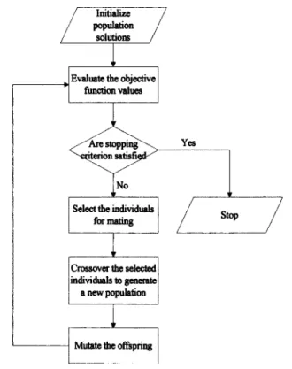
using 1 / L or 0.001 as the probability of mutation. Fig. 1 shows the flowchart for the GA approach. After selecting the initial guesses, the trial solution, determined by the optimal fitness func-tion value, will proceed to the crossover step. In addifunc-tion to the crossover step, each bit in the newborn trial solution, the binary string, will be mutated depending on the mutation probability. The algorithm will be terminated when the solution or the number of iterations satisfies the stopping criteria.
Simulated Annealing
The concept of SA is based on an analogy with the physical annealing process. In the beginning of the process, the tempera-ture is increased to enhance the molecular mobility. Next, the temperature is slowly decreased to allow the molecules to form crystalline structures. When the temperature is high, the mol-ecules have a high level of activity and the crystalline configura-tions assume a variety of forms. If the temperature is lowered properly, the crystalline configuration is in the most stable state; thus, the minimum energy level may be naturally reached.
At a given temperature, the probability distribution of the
sys-tem energy is determined by the Boltzman probability共Pham and
Karaboga 2000兲:
P共E兲 ⬀ exp共− E/kT兲 共13兲
where E⫽system energy; k⫽Boltzmann’s constant;
T⫽temperature; and P共E兲⫽occurrence probability. There exists a
small probability that the system may have high energy even at low temperature. Therefore, the statistical distribution of energies allows the system to escape from a local minimum energy. This is the major reason why the solutions obtained from SA may not become trapped as a local optimum or result in a poor solution. The Boltzmann probability is applied in Metropolis’ criterion 共Kirkpatrick et al. 1983兲 to establish the probability distribution function for the trial solution. The Metropolis’ criterion takes the
place ⌬E, the difference between the current solution and trial
solution of E, and k being equal to one. The modified Boltzmann probability which represents the probability that the trial solution will be accepted is given as
P共⌬E兲 = exp共⌬E/T兲 共14兲
As an iterative improvement method, an initial point x is
re-quired to evaluate the objective function value f共x兲. Let x⬘assume
the position as the neighbor of x and its objective function value is f共x⬘兲. In the minimization problem, if f共x⬘兲 is smaller than f共x兲,
then the trial solution共x⬘兲 takes the place of the current optimal
solution共x兲. If f共x⬘兲 is not smaller than f共x兲, then one has to test
Metropolis’s criteria and generate a new random number D be-tween zero and one. For solving minimization problems, the
Me-tropolis’s criterion is given as共Metropolis et al. 1953兲:
PSA兵accept j其 =
冦
1 if f共j兲 艋 f共i兲 exp
冉
f共i兲 − f共j兲T
冊
if f共j兲 ⬎ f共i兲冧
共15兲
where f共i兲 and f共j兲 are, respectively, the function value when x
= xiand x = xj. xiand xjare, respectively, the current optimal
so-lution and neighborhood trial soso-lution of x. Here T, a control parameter, is usually the current temperature. For solving the maximization problem, Metropolis’s criterion is expressed as
PSA兵accept j其 =
冦
1 if f共j兲 ⬎ f共i兲 exp
冉
f共j兲 − f共i兲T
冊
if f共j兲 艋 f共i兲冧
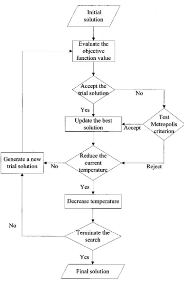
共16兲 Fig. 2 displays the SA algorithm approach. The first step in SA is to initialize a solution and set the initial solution to equal the current optimal solution. The second step is to update the current optimal solution, if the trial solution generated from the initial solution within the boundary is better than the current optimal solution; otherwise, continue generating trial solutions until the algorithm satisfies the temperature decrease criterion. The algo-rithm will be terminated when SA obtains the optimal solution or the obtained solution satisfies the stopping criteria. In general, the stopping criteria are defined to check whether the temperature or the iteration number reaches the specified value or not.
Two modifications to the SA approach are introduced in this study to ensure that the solutions obtained from SA are the opti-mum solutions. In the first modification, the Metropolis criterion is expressed as
Fig. 1.Flowchart of genetic algorithm
PSA兵accept j其 =
冦
1 if f共j兲 艋 f共i兲 exp
冋
冉
f共i兲 − f共j兲f共j兲
冊
/T册
if f共j兲 ⬎ f共i兲冧
共17兲 This modified criterion is different from the general Metropolis
criterion as mentioned previously. In Eq.共17兲, the increment
be-tween the current best solution and the neighborhood trial solu-tion is divided not only by parameter T, but also by the neighbor-hood trial solution. After the temperature decreases several times, any acceptance probability obtained from the modified Metropolis criterion will be smaller than that obtained from the general Me-tropolis criterion. The best solution obtained from the modified Metropolis criterion will converge much faster than that using the general Metropolis criterion because unfavorable solutions will not be accepted in the algorithm.
The second modification is to adjust the searching number
with a factor for decreasing temperature. In general,  is given
as 1.1 共Cunha and Sousa 1999兲. Due to an increasing of the
searching number, more trial solutions will be created and a much higher possibility will be achieved to obtain the optimal solution. In addition, Fig. 3 shows a brief schematic explaining how to apply GA and/or SA coupled with the kinetics of THM and THM species to forecast the THM species concentrations, and proce-dure is given in the following steps:
1. Initialize the initial guesses and the BIF value obtained from
prior experimental results.
2. Calculate the TTHM and THM3 concentrations based on
Eqs.共4兲 and 共5兲.
3. Apply GA or SA to analyze the THM0, THM1, and THM2
concentrations. Note that the algorithmic parameters in GA or SA need to be specified in this step.
4. Check the obtained results. If the trial solutions do not satisfy
the stopping criterion, go back to Step 3 to keep on generat-ing the possible solutions. Otherwise, the algorithm is termi-nated.
Case Study and Results
The finished water system in Alain, United Arab Emirates 共Elshorbagy 2000兲 was chosen as the study case for this experi-ment. Water was injected with chlorine from the pumping station to maintain a residual level from 0.3 to 0.5 ppm prior to pumping into the Alain distribution system. The bromide levels in the fin-ished water ranged between 0.1 and 0.4 ppm. A prior experiment recorded the variation of parameters such as total organic carbon and pH with time. The experimental results indicated that those parameters are approximately constant with respect to time. Based on the experimental results, BIF was also concluded to be a constant. This assumption provides a basis for the development of the modeling approach.
In this study, Kcl, F, and kbwere, respectively, taken as 0.070,
0.706, and 0.121 1 / h, and the concentrations of 关Br0兴 and 关Bru兴
were, respectively, 2.6 and 8.2g/L 共Elshorbagy 2000兲. In the
GA approach, several parameters are needed to be assumed at the beginning. Each unknown was encoded into a 24-bit binary
string. Other parameters such as population size, Pc, and Pm, were
given as 20, 0.6, and 1 / L, i.e., 1 / 72, respectively. After 5,000 generations, the GA approach was terminated.
Fig. 2.Flowchart of simulated annealing关adapted from Pham and Karaboga共2000兲兴
Fig. 3.Schematic diagram of the forecasting procedure
When using the SA approach, four different cases for deter-mining the THM concentrations were considered. Due to the ran-dom number generator needs two seeds to generate the ranran-dom number, Cases 1 and 2 employed different random number seeds for the SA. The random number seeds used in Case 1 were one and two and in Case 2 were three and four, since SA requires two seeds to generate a series of random numbers. Case 3 used the
modified Metropolis criteria, Eq.共17兲, and Case 4 used a variable
searching number, which increased with a multiplication factor 1.1 as the temperature is decreased.
In Case 3, the acceptance probability decreased with decreas-ing temperature. Thus the solutions obtained at the last step were
better than those of the previous steps. In Case 4, the searching number increased upon decreasing the temperature and naturally resulted in increasing the number of trial solutions. The probabil-ity of obtaining the global optimum was then increased. Note that all parameters such as reducing temperature factor, initial tem-perature, initial guesses, and error tolerance were kept all the same in Cases 1–4. The initial temperature and reducing tempera-ture factor were, respectively, taken as 5 and 0.8 in Cases 1–4. The algorithm was terminated when the difference between the current best solution and last step best solution became less than
10−6in 12 iterations. After 1,200 iterations, the temperature was
decreased in Cases 1–3.
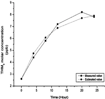
The calculated concentrations of TTHM from Eq. 共4兲 and
THM3from Eq.共5兲 are given in Figs. 4 and 5, respectively. The
concentrations of THM0, THM1, and THM2were obtained from
experiment and simulations at different times throughout one day.
The temporal concentration distributions of THM0, THM1, and
THM2 listed in Table 1 show that the calculated values are not
significantly different from the measured ones. Also, the THM0
concentrations obtained from heuristic methods are shown to be very close to the experimental and GRG2 values. However, the
concentrations of THM1and THM2obtained from GA and SA are
slightly different than compared to those obtained from GRG2.
Note that the measured values of S1and S3at 8, 12, and 20 h
listed in Table 2 do not satisfy the constraint of Eq.共10兲. This may
be the major reason why the calculated concentrations of THM2
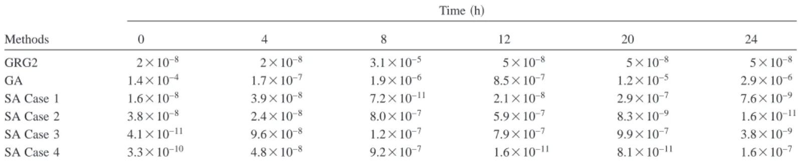
and THM3differ from the measured ones. The objective function
values of Eq. 共12兲 versus time obtained from the GRG2 model,
GA, and SA are demonstrated in Table 3. Note that the values at different times for SA Cases 1, 2, and 3 are roughly the same, and the values obtained from SA Case 4 are much better than those of the GRG2 model. Although the objective function values obtained from GA are not better than those obtained from GRG2, the THM species concentrations obtained from GRG2 and GA do not show a significant difference.
Fig. 6 exhibits the THM1, THM2, and THM3concentrations
obtained from SA while employing values of 0.1, 1, and 10 for the Lagrange multiplier. The estimated concentrations for each species are not significantly different, implying that the first term
of Eq. 共12兲 dominates the calculation. In this study, the
concen-trations of THM species are estimated with a constant BIF. In
reality, the values of BIF can be calculated using Eq.共6兲 with the
measured concentrations of the THM species, indicating that the calculated BIF slightly varied with time. The BIF values
calcu-lated from Eq.共6兲 at 0, 4, 8, 12, 20, and 24 h are 0.7303, 0.7453,
0.7309, 0.7287, 0.723, and 0.7526, respectively 共Elshorbagy
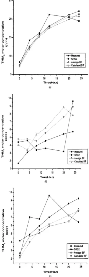
2000兲. However, Fig. 7 indicates that the four estimated THM concentrations based on the average BIF value and the calculated BIF values do not show a considerable difference. Thus, assum-ing that BIF is a constant is reasonable and practical in the THM estimations. Note that the maximum computing time is about 6.83 s for SA and 7.27 s for GA when simulating the THM con-centrations on a personal computer with Intel PIII-800 CPU.
Conclusions and Future Study
Chlorination is a commonly used method for disinfection in the water distribution system. The purpose of disinfection is to re-move the water-borne disease for providing healthy drinking water. However, chlorine reacts with the organic or inorganic ma-terials to produce THM. In recent years, some studies indicate that the THM species are the carcinogens.
Fig. 4. Temporal concentration distributions of the measured and estimated total trihalomethanes
Fig. 5. Temporal concentration distributions of the measured and estimated bromoform
Table 1.Measured and Modeled Values for Chloroform共THM0兲, Bromodichloromethane 共THM1兲, and Dibromochloromethane 共THM2兲 Species Con-centrations共ppb兲 at Different Times
Time共h兲 Method 0 4 8 12 20 24 共a兲 THM0 Experiment 7.4 14.2 16.2 21.2 20.4 19.4 GRG2 8.35 12.56 15.73 18.08 21.11 22.07 GA 8.26 12.26 15.51 18.12 21.04 21.48 SA Case 1 7.30 12.11 15.62 17.64 20.18 20.61 SA Case 2 7.49 12.44 15.20 17.49 19.88 21.32 SA Case 3 7.18 12.03 15.52 17.45 19.93 20.87 SA Case 4 7.86 12.49 15.38 17.98 20.96 21.97 共b兲 THM1 Experiment 4.4 4.6 3.4 3.6 3.2 9.6 GRG2 1.69 3.08 3.94 4.56 5.43 5.73 GA 1.69 3.90 4.54 4.48 5.82 7.40 SA Case 1 4.58 4.30 4.25 5.79 8.02 9.72 SA Case 2 4.05 3.41 5.36 6.21 8.81 7.79 SA Case 3 4.89 4.52 4.52 6.33 8.65 9.03 SA Case 4 3.05 3.28 4.87 4.83 5.86 5.98 共c兲 THM2 Experiment 2.4 7 6.8 9.6 7.2 6.4 GRG2 4.19 4.93 5.96 6.99 8.63 9.24 GA 4.33 4.40 5.55 7.05 8.27 8.12 SA Case 1 2.37 4.15 5.77 6.19 6.96 6.70 SA Case 2 2.69 4.71 5.08 5.91 6.48 7.92 SA Case 3 2.16 4.02 5.58 5.87 6.61 7.14 SA Case 4 3.33 4.80 5.39 6.81 8.35 9.09
Note: GRG2⫽generalized reduced gradient method; GA⫽genetic algorithm; and SA⫽simulated annealing .
Table 2.Measured Bromine Distribution Factor共BDF兲 at Different Times
Measured BDF Time共h兲 0 4 8 12 20 24 S0 0.5599 0.6004 0.6398 0.6475 0.6635 0.5747 S1 0.2427 0.1418 0.0979 0.0802 0.0759 0.2073 S2 0.1042 0.1698 0.1541 0.1682 0.1343 0.1088 S3 0.0930 0.0880 0.1083 0.1040 0.1261 0.1093
Table 3.Temporal Values of the Objective Function Calculated Based on Eq.共12兲
Methods Time共h兲 0 4 8 12 20 24 GRG2 2⫻10−8 2⫻10−8 3.1⫻10−5 5⫻10−8 5⫻10−8 5⫻10−8 GA 1.4⫻10−4 1.7⫻10−7 1.9⫻10−6 8.5⫻10−7 1.2⫻10−5 2.9⫻10−6 SA Case 1 1.6⫻10−8 3.9⫻10−8 7.2⫻10−11 2.1⫻10−8 2.9⫻10−7 7.6⫻10−9 SA Case 2 3.8⫻10−8 2.4⫻10−8 8.0⫻10−7 5.9⫻10−7 8.3⫻10−9 1.6⫻10−11 SA Case 3 4.1⫻10−11 9.6⫻10−8 1.2⫻10−7 7.9⫻10−7 9.9⫻10−7 3.8⫻10−9 SA Case 4 3.3⫻10−10 4.8⫻10−8 9.2⫻10−7 1.6⫻10−11 8.1⫻10−11 1.6⫻10−7 Note: GRG2= generalized reduced gradient method; GA= genetic algorithm; and SA= simulated annealing.
Fig. 6. 共a兲 Chloroform concentration; 共b兲 bromodichloromethane
concentration; and共c兲 dibromochloromethane concentration obtained from simulated annealing when different values of the Lagrange mul-tipliers are employed
Fig. 7.Three trihalomethane species concentration calculated based on average bromine incorporation factor共BIF兲 and estimated calcu-lated BIF. 共a兲 Temporal concentration of chloroform concentration;
共b兲 temporal concentration of bromodichloromethane
concen-tration; and 共c兲 temporal concentration of dibromochloromethane concentration
Heuristic methods, developed very rapidly in recent years, are wildly employed in the research field. Both GA and SA were used to calculate the concentrations of THM species in desalinated water. The control parameters in the kinetics of THM species are
the chlorine demand–关TTHM兴 growth coefficient, the bromoform
reaction rate coefficient, and the average representative bromine incorporation. The present approach incorporates necessary con-straints, such as the bromine distribution factor and BIF factor, in the optimization formulation as a means of better representation of the site-specific water quality characteristics.
The heuristic approaches of GA, general SA, and two modified SAs are employed to solve this optimization problem. These ap-proaches have the merit of arbitrarily choosing the initial guess and, still, can obtain reasonably good results. The calculated con-centrations of THM species by GA and SA differed from the measured values, yet those results satisfied the constraints of the species mass balance and are in close agreement with those re-sults obtained from GRG2.
In this study, the objective function values obtained from GA are slightly inferior to those of GRG2. Yet, the calculated THM species concentrations obtained from GA do not differ signifi-cantly from GRG2. In Cases 1 and 2 of the SA approach, most results obtained from SA were about the same order of magnitude as those of GRG2. However, some values were better than those of GRG2. In Case 4, SA provides better results than those of GRG2 in terms of the objective function values. This indicates that increasing the searching number with decreasing temperature may yield better results.
The approach of using GA or SA coupled with the THM for-mation kinetic equations might provide a useful tool for analyzing the concentration of THMs and facilitate the ability of water qual-ity management.
For problems where traditional approaches, such as gradient-type solvers or programming techniques, fail to obtain the optimal solution, the heuristic approaches might be an alternative. The future study for forecasting the quality of drinking water might include developing an online monitoring system to assure the safety of water usage. In addition, applying the heuristic ap-proaches to identify the model parameters is also one of our on-going researches.
Acknowledgment
This study was partially financially supported by the National Science Council of Taiwan under Grant No. NSC90-2621-009-003.
Notation
The following symbols are used in this paper:
BIF ⫽ bromine incorporation factor;
E ⫽ system energy;
F ⫽ linear proportionality constant between total
trihalomethane and chlorine;
Kb ⫽ bromoform reaction rate coefficient;
Kcl ⫽ chlorine reaction rate coefficient;
k ⫽ Boltzmann’s constant; L ⫽ total string length; li ⫽ substring length;
Pc ⫽ crossover probability;
Pm ⫽ mutation probability;
PSA ⫽ acceptance probability that when the trial
solution doesn’t better than the current best solution;
P共E兲 ⫽ occurrence probability when the system and
temperature are E and T, respectively; S0, S1, S2, S3 ⫽ bromine distribution factors of chloroform,
bromodichloromethane, dibromochloromethane, and bromoform, respectively;
T ⫽ temperature;
关x兴 ⫽ x species concentration; and ⫽ Lagrange multiplier.
References
Aarts, E., and Korst, J.共1989兲. Simulated annealing and Boltzmann ma-chines: A stochastic approach to combinatorial optimization and neu-ral computing, Wiley, New York.
Adin, A., Katzhendler, J., Alkaslassy, D., and Ravacha, C.共1991兲. “Tri-halomethane formation in chlorinated drinking water—A kinetic model.” Water Res. 25共7兲, 797–805.
Amy, G. L., Chadick, P. A., and Chowdhury, Z. K.共1987兲. “Developing models for predicting trihalomethane formation potential and kinet-ics.” J. Am. Water Works Assoc., 79共7兲, 90–97.
Bitton, G.共1999兲. Wastewater microbiology, Wiley, New York. Bunn, W. W., Haas, B. B., Deane, E. R., and Kleopfer, R. D.共1975兲.
“Formation of trihalomethanes by chlorination of surface waters.” En-viron. Lett., 10共3兲, 205.
Clark, R. M.共1998兲. “Chlorine demand and THM formation kinetics: A second-order model.” J. Environ. Eng. 124共1兲, 16–24.
Clark, R. M., Smalley, G., Godrich, J., Tull, R., Rossman, L. A., Vascon-celos, J. J., and Boulus, P. F. 共1994兲. “Managing water quality in distribution systems: Simulating TTHM and chlorine residual pro-gram.” J. Water SRT-Aqua, 43共4兲, 182–191.
Coley, D. A.共1999兲. An introduction to genetic algorithms for scientists and engineers, World Scientific, Arbid, Mass.
Cunha, M. D. C., and Sousa, J.共1999兲. “Water distribution network de-sign optimization: Simulated annealing approach.” J. Water Resour. Plan. Manage. 125共4兲, 215–221.
Domer, B., Raphael, B., Shea, K., and Smith, I. F. C.共2003兲. “A study of two stochastic search methods for structure control.” J. Comput. Civ. Eng. 17共3兲, 132–141.
Elshorbagy, W. E.共2000兲. “Kinetic of THM species in finished drinking water.” J. Water Resour. Plan. Manage. 126共1兲, 21–28.
Goffe, W. L., Ferrier, G. D., and Rogers, J.共1994兲. “Global optimization of statistical functions with simulated annealing.” J. Econometr.
60共1兲, 65–100.
Golfinopoulos, S. K., Xilourgidis, N. K., Kostopoulou, N., and Lekkas, T. D.共1998兲. “Use of a multiple regression model for predicting triha-lomethane formation.” Water Res. 32共9兲, 2821–2829.
Gould, J. P., Fitchhorn, L. E., and Urheim, E. 共1981兲. “Formation of brominated trihalomethanes: Extent and kinetics.” Water chlorination: Environment impacts and health effects, Vol. 4, R. L. Jolley et al., eds., Ann Arbor Science, Ann Arbor, Mich., 297–310.
Gupta, I., Gupta, A., and Khamma, P. 共1999兲. “Genetic algorithm for optimization of water distribution systems.” Environ. Modeling, Soft-ware, 14共5兲, 437–446.
Gwo, J. P. 共2001兲. “In search of preferential flow paths in structured porous media using a simple genetic algorithm.” Water Resour. Res.
37共6兲, 1589–1601.
Hillier, F. S., and Lieberman, G. J. 共1990兲. Introduction to operations research, 5th Ed., McGraw-Hill, New York.
Holland, J.共1975兲. Adaptation in natural and artificial system, University Press, Cambridge, Mass.
Kirkpatrick, S., Gelatt, C. D., Jr., and Vecchi, M. P.共1983兲. “Optimization by simulated annealing.” Science, 220共4598兲, 671–680.
Lasdon, L. S., and Warren, A. D.共1982兲. GRG2 user’s guide, Dept. of General Business, Univ. of Texas at Austin, Tex.
Lippai, I., Heaney, J. P., and Laguna, M.共1999兲. “Robust water system design with commercial intelligent search optimizers.” J. Comput. Civ. Eng. 13共3兲, 135–143.
McKinney, D. C., and Lin, M. D.共1994兲. “Genetic algorithm solution of groundwater management models.” Water Resour. Res. 30共6兲, 1897– 1906.
Metropolis, N., Rosenbluth, A. W., Rosenbluth, M. N., Teller, A. H., and Teller, E.共1953兲. “Equation of state calculations by fast computing machines.” J. Chem. Phys. 21共6兲, 1087–1092.
Milot, J., Rodriguez, M. J., and Serodes, J. B.共2002兲. “Contribution of neural networks for modeling trihalomethanes occurrence in drinking water.” J. Water Resour. Plan. Manage. 128共5兲, 370–376.
Minear, R. A.共1980兲. “Production, fate and removal of trihalomethanes in municipal drinking water systems.” Res. Rep. No. 78, Tennessee Water Research Center, Knoxville, Tenn.
Montogomery Watson.共1993兲. “Mathematical modeling of the formation of THMs and HAAs in chlorinated natural waters.” Final Rep. sub-mitted to the AWWA Disinfectant/Disinfection By-Products Technical Advisory Workgroup, American Water Works Association, Denver. Nokes, C. J., Fenton, E., and Randall, C. J.共1999兲. “Modeling the
for-mation of brominated trihalomethanes in chlorinated drinking wa-ters.” Water Res. 33共17兲, 3357–3568.
Pham, D. T., and Karaboga, D. 共2000兲. Intelligent optimization tech-niques, Springer, U.K.
Rook, J. J.共1974兲. “Formation of haloforms during chlorination of natu-ral waters.” Water Treat. Exam., 23, 234–243.
Trussel, R. R., and Umphres, M. D.共1978兲. “The formation of trihalom-ethanes.” J. Am. Water Works Assoc., 70共11兲, 604–612.
Youssef, H., Sait, S. M., and Adiche, H.共2001兲. “Evolution algorithms, simulated annealing and tabu search: A comparative study.” Eng. Ap-plic. Artif. Intell. 14, 167–181.