SOME PROCESS CAPABILITY INDEXES ARE MORE RELIABLE THAN ONE MIGHT THINK

Some Process Capability Indices are More Reliable than One Might Think

Author(s): Samuel Kotz, Wen Lea Pearn and N. L. Johnson

Source: Journal of the Royal Statistical Society. Series C (Applied Statistics), Vol. 42, No. 1

(1993), pp. 55-62

Published by:

Wiley

for the

Royal Statistical Society

Stable URL:

http://www.jstor.org/stable/2347409

.

Accessed: 28/04/2014 13:37

Your use of the JSTOR archive indicates your acceptance of the Terms & Conditions of Use, available at

.

http://www.jstor.org/page/info/about/policies/terms.jsp

.

JSTOR is a not-for-profit service that helps scholars, researchers, and students discover, use, and build upon a wide range of

content in a trusted digital archive. We use information technology and tools to increase productivity and facilitate new forms

of scholarship. For more information about JSTOR, please contact support@jstor.org.

.

Wiley and Royal Statistical Society are collaborating with JSTOR to digitize, preserve and extend access to

Journal of the Royal Statistical Society. Series C (Applied Statistics).

42, No. 1, pp. 55-62

Some Process Capability Indices are More

Reliable than One Might Think

By SAMUEL KOTZt

University of Maryland, College Park, USA WEN LEA PEARN

National Chiao Tung University, Hsin Chu, Republic of China and N. L. JOHNSON

University of North Carolina, Chapel Hill, USA [Received January 1991. Revised August 19911 SUMMARY

In this paper we obtain formulae for exact expected values and standard deviations of estimators of certain process capability indices discussed by Bissell. In particular, we show that for the index Cpk

Bissell's formula gives values for the standard deviation which are too high especially when the actual population mean value is close to (or equal to) the average of the upper and lower specification limits. Keywords: Capability indices; Non-central x -distribution; Standard error; Stirling approximation

1. Introduction

Process

capability

indices

(PCIs) (whose

purpose

is to provide

a numerical

statement

of the extent

to which

the output

of a process

satisfies

a preassigned

specification)

have received

substantial

attention

in statistical

and quality

control

publications

in

recent

years.

Most prominenitly,

Kane (1986) provides

a thorough

discussion

and lucid

comparison

of five basic capability

indices

(Cp, CPU, CPL, k and

Cpk)

which

were

developed

in British

and European,

American

and Japanese

quality

control

branches

of industrial

and engineering

institutions

with

special

attention

to the Japanese

CPU

and Cp indices

popularized

by Sullivan

(1984). Recently,

Chan

et al.

(1988) proposed

and investigated

some distributional

properties

of a new measure

of process

capability

Cpm

to take into account

the proximity

to target

as well as the process

variation

in the

assessment

of process performance

based on a Bayesian approach. Porter and

Oakland (1990) advocate

the construction

of confidence

intervals

for

the basic indices

Cp and

Cpk.

Most of the investigations

depend

heavily

on the underlying

assumption

of normal

variability,

although

an attempt

to extend

the results

available for non-

normal

distributions

using

the Pearson

family

of probability

curves

has recently

been

tAddress for correspondence: College of Business and Management, University of Maryland, College Park, MD 20742, USA.

56

KOTZ, PEARN AND JOHNSON

made by Clements

(1989). Finally Bissell (1990) obtained simple but efficient

approximate

formulae

for

the variances

of several

PCIs. Among

the PCIs considered

by Bissell

are

USL-LSL

CP

_6cr

6a

(1)

and

Cpk

=

min(

USL

LSL)

(2)

where

USL and LSL denote

the upper and lower specification

limits

respectively,

₁₄

denotes

the process

mean and ar

the process

standard

deviation.

Estimators

of these

PCIs can be obtained

by replacing

₁₄

and ar

by the estimators

j4 and a respectively.

2. Distribution

On the basis of a normal

distribution

of measured

characteristics.

Bissell con-

sidered

two types

of estimator

of a:

(a) the sample standard deviation

S

=

{(n-1)-i

-(X)2}112

where X=

n-l = IXi and

(b) the range (or mean range of subsamples)

multiplied

by an appropriate

unbiasing

factor.

In case (a) S2 is distributed

as (n -

1)-

1cr2

times

a x2-variable

with

n - 1 degrees

of

freedom-symbolically,

S2

(n

-

_1)-nlX

1cr2;

in case (b)

o2

is

distributed

approximately

_{asf - fXc2}

where

f is an appropriate

constant

depending

on n.

The process

_{mean 14}

is estimated

by X. On the assumption

of normality,

X and

S2,

or cr

,

are mutually

independent,

even if based (as is usual) on the same sample.

The numerator

of

Cpk

can be written

as d -

1

- 01 where d

=

2(USL

- LSL) and

0 = ₂

(USL + LSL). Hence we consider

the estimator

Cpk

=

d-

IX-lol d(

1 IX-Lo/ln)/ 3xf

₍₃₎

On the assumption

of a normal

distribution,

Xf

and IX- o

I

'In/ca

are indepen-

dently

distributed.

The statistic

I

X- tto

_I

In/ca

has a folded normal

distribution

as

defined

by Leone et

al.

(1961). From the results

of this paper (see also Johnson

and

Kotz (1970)) we have

E(

[XLoI')

=V(2)

exp

_{23

+

I

oln t1-24(-

A O

,

_(4a)

where

u

and

E

_(?IX-toI)}1 =1 +4( 2 (4b)

The distribution

of

Cpk

depends on the parameters

_{dia and 114}

-

_IA4In.

The rth

moment

about 0 of

Cpk

is

E(Cpk) = (f) E( )

(I

1)

)

(a)r(1)IE{(

_aI)I}

whence

E(Cpk)

1()

-[L

J(i)

ex

2p(

o

3

2

t

b(

a

)3rn

2

)

2)(a

and

var(Cpk) -

_9(f

_-2)\\or

((-)-2(-)

_\or

d

(-ex)

_7r

x2

_2or

3

+

I

{ 2(

ao

) 2

+3

_E(cpk)2])

(b)

Expressions

(5a) and (5b) are equivalent

to those

obtained

by Zhang et al. (1990) by

using

a different

method,

without

obtaining

the actual distribution

of

cpk.

Dr Zhang

has told us that his numerical

calculations

coincide

with

ours.

If we use

n 1/2

a=S=

(n-1)Yj(xj_X)2

j=l

thenf=

n -

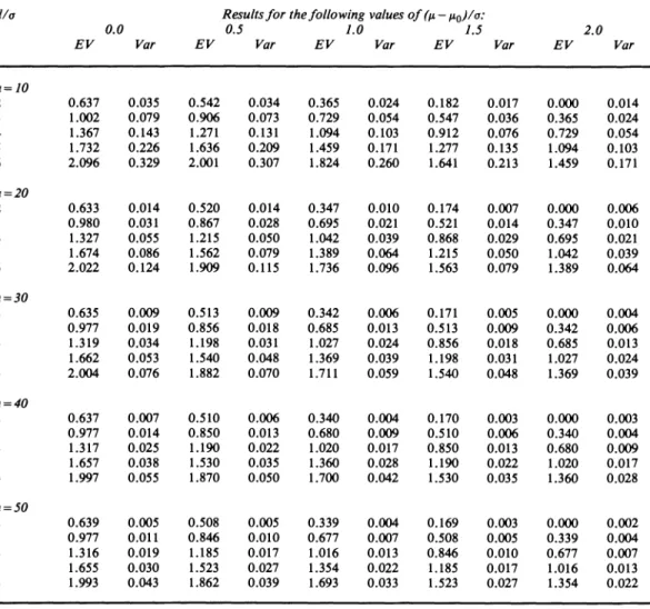
1. Some numerical

values

of

E(Cpk)

and

var(Cpk)

are presented

in

Table 1.

We urge the reader

to examine

the column

corresponding

to

s4

= 140

most carefully.

Corresponding

values of

Cpk

are presented

in Table 2.

Cpk

is

a biased estimator

of

Cpk.

The bias arises

from

two sources:

(a)

E(

)

=J(i)F(ff

r

o2)r

/

(2)

(this bias is positive);

(b)

E ( -

_or

>olAn

4-H I

_a

(this leads to negative bias since IX-to

I

In/l has a negative sign in the

numerator

of

Cpk).

The resultant

bias is positive

for all cases shown

in Table 1 for which

1 * y0. When

58

KOTZ, PEARN AND JOHNSON TABLE 1

Moments of Cpkt

dia _{Results for the following values of (A - Ao)/o:}

0.0 0.5 1.0 1.5 2.0 EV Var EV Var EV Var EV Var EV Var

n=10 2 0.637 0.035 0.542 0.034 0.365 0.024 0.182 0.017 0.000 0.014 3 1.002 0.079 0.906 0.073 0.729 0.054 0.547 0.036 0.365 0.024 4 1.367 0.143 1.271 0.131 1.094 0.103 0.912 0.076 0.729 0.054 5 1.732 0.226 1.636 0.209 1.459 0.171 1.277 0.135 1.094 0.103 6 2.096 0.329 2.001 0.307 1.824 0.260 1.641 0.213 1.459 0.171 n =20 2 0.633 0.014 0.520 0.014 0.347 0.010 0.174 0.007 0.000 0.006 3 0.980 0.031 0.867 0.028 0.695 0.021 0.521 0.014 0.347 0.010 4 1.327 0.055 1.215 0.050 1.042 0.039 0.868 0.029 0.695 0.021 5 1.674 0.086 1.562 0.079 1.389 0.064 1.215 0.050 1.042 0.039 6 2.022 0.124 1.909 0.115 1.736 0.096 1.563 0.079 1.389 0.064 n =30 2 0.635 0.009 0.513 0.009 0.342 0.006 0.171 0.005 0.000 0.004 3 0.977 0.019 0.856 0.018 0.685 0.013 0.513 0.009 0.342 0.006 4 1.319 0.034 1.198 0.031 1.027 0.024 0.856 0.018 0.685 0.013 5 1.662 0.053 1.540 0.048 1.369 0.039 1.198 0.031 1.027 0.024 6 2.004 0.076 1.882 0.070 1.711 0.059 1.540 0.048 1.369 0.039 n =40 2 0.637 0.007 0.510 0.006 0.340 0.004 0.170 0.003 0.000 0.003 3 0.977 0.014 0.850 0.013 0.680 0.009 0.510 0.006 0.340 0.004 4 1.317 0.025 1.190 0.022 1.020 0.017 0.850 0.013 0.680 0.009 5 1.657 0.038 1.530 0.035 1.360 0.028 1.190 0.022 1.020 0.017 6 1.997 0.055 1.870 0.050 1.700 0.042 1.530 0.035 1.360 0.028 n =50 2 0.639 0.005 0.508 0.005 0.339 0.004 0.169 0.003 0.000 0.002 3 0.977 0.011 0.846 0.010 0.677 0.007 0.508 0.005 0.339 0.004 4 1.316 0.019 1.185 0.017 1.016 0.013 0.846 0.010 0.677 0.007 5 1.655 0.030 1.523 0.027 1.354 0.022 1.185 0.017 1.016 0.013 6 1.993 0.043 1.862 0.039 1.693 0.033 1.523 0.027 1.354 0.022 tf= n - 1; EV, expected value; Var, variance.

TABLE 2 Values of Cp k

dia _{Results for the following values of (I - It)/a:} 0.0 0.5 1.0 1.5 2.0 2.0 2 1 1 1 0 3.0 3.0

~

_~~~

1 ₁ 3 _{5 2} 1 1 4.0 1. 11 1 6 2 5.0 12 ₃ 1 ₂ 1! ₃ 1 ₆ 1 6.0 2 1 5121

TABLE 3

Values of E(Cp k) for u = IO and dla = 3 corresponding to CP k = I for a series of increasing values of n

Sample size n E(Cpk) Sample size n E(Cpk)

10 1.002 600 0.990 20 0.980 2200 0.995 30 0.977 3200 0.996 60 0.978 5400 0.997 80 0.980 10800 0.998 100 0.981 30500 0.999 200 0.985 79500 1.000 400 0.989

of 3.0 and 4.0 it is negative

for all n

)

20, for d/uf=

5.0 for n

)

30, and for dia

=

6.0

for n ? 40.) Ultimately,

as n

-+ oo

the bias tends to 0.

This is explored in more detail in Table 3 which presents

the values of

E(Cpk)

for

(tt - AO)Ia = 0 and dla = 3 (in this case the 'theoretical'

value of Cpk is 1). An explicit

formula in this case for

E(Cpk)

is easily seen to be

E(Cpk)

3{ +

1

(irn)3 \( 2 )F( 2 ) F/F( 2 )

(6)

For our calculations we have used this exact formula together

with an approximate

formula

in which the ratio of the gamma functions

was approximated

via the Stirling

formula by

r

n-2)r(

2 1

/(2 ) l-4(n - 2) + _32(n

-

₂₎₂

_{128(n -}

_{2) 3}

The values of E(Cpk) calculated by using these two formulae coincide (up to the

fourth

decimal place) for the values of n presented

in Table 3, which indicates

the high

accuracy of the Stirling

approximation

used.

3. Comments on Bissell's Modification

Although Bissell (1990) defines

Cpk as in equation (2), in the later part of this paper

he uses the estimator

USL-X

(7a)

or

CPk

=

X-LSL

(7b)

according to whether

_s4

is greater

_{than or less than 1 (USL + LSL) = 140.}

As Bissell notes, in either case the distribution

of 3CpkVn is non-central

t with

f

degrees

of freedom

and non-centrality

parameter

(d - 14 - AO

I

)VIn. We shall consider,

without loss of generality,

_{ti > 140.}

It is to be expected that

C,k

will have a greater

60 KOTZ, PEARN AND JOHNSON

variance

than

?pk

because, when X

>

L0,

Cpk= Cpk,

however,

when X

<

4 the

numerator

of

Cpk

is greater

(by 2(AO

-

X)) than that

of

_Cpk.

For the same reason,

we

expect

E(Cpk)

to exceed

E(Cpk),

leading to greater

positive

bias when 4 * y0.

However,

these

effects

will not be large (except

when

₁₄

differs

little

from

_{uo) because}

the probability

prob(X <

AO) =

4

(D

ItLtLoLl)

is indeed

quite small, except

for small values of n.

The most

noticeable

effect

will be the reduction

in the variance

when

t

=

40 (which

serves

as a justification

of the title

of this paper).

The expected

value of

Cpr

is

E(Cp'r)k

E{(d-X+fo)r}

3r

E(Xf)r'

In particular

E(Cpk)=

_3(2jf)

_(a

)rf

_{2 2)/F(2)}

(8a)

(compare equation (5a)) and

var(CGk)

=

9

f-2{

(d

-

a ) +

- _E(Cpk)2*

(8b)

For 4

=

40 we find that

E(Cpk)

=

_E(Cpk){1

-

(d)\/(3n)

}-

and

var(Cpk) = var(Cpk) -

a[f-2

_J {

2(f21)

/

2(f)]

9

in

r

2 r/

(2

<var(Cpk), since

r

2 )(2)

fr-2.

(Note that

r2(z) <

r(z

-

I) r(z +2).)

Bissell

(1990) obtains

an approximate

formula

for

var(C,k)

by using

the method

of

statistical

differentials.

It is (in our notation)

C2(var(d

-X + so)

var(o&).1

+

Cfk

var(Cpk)

pk

₊

₁₂₎ +

2-3

_(8C)

(d -is+o

a

9n 2f

(c

(This formula

does not allow for bias in

C0k

as an estimator

_{of Cpk; however,}

the

effect

of this will be of a higher

order

in

n-

I orf- 1.)

TABLE 4

Moments of C0,t

dla Results for the following values of (1i - l0)/o:

0.0 0.5 1.0 1.5 2.0 EV Var EV Var EV Var EV Var EV Var

n=10 3 1.094 0.103 0.912 0.076 0.729 0.054 0.547 0.036 0.365 0.024 4 1.459 0.171 1.277 0.135 1.094 0.103 0.912 0.076 0.729 0.054 5 1.824 0.260 1.641 0.213 1.459 0.171 1.277 0.135 1.094 0.103 6 2.188 0.368 2.006 0.311 1.824 0.260 1.641 0.213 1.459 0.171 n =20 3 1.041 0.048 0.868 0.029 0.694 0.021 0.521 0.015 0.347 0.010 4 1.388 0.065 1.215 0.052 1.041 0.048 0.868 0.029 0.694 0.021 5 1.736 0.099 1.562 0.081 1.388 0.065 1.215 0.052 1.041 0.048 6 2.083 0.139 1.909 0.118 1.736 0.099 1.562 0.099 1.388 0.065 n =30 3 1.027 0.024 0.855 0.019 0.685 0.013 0.513 0.009 0.342 0.006 4 1.369 0.039 1.198 0.031 1.027 0.024 0.855 0.018 0.685 0.013 5 1.711 0.059 1.540 0.048 1.369 0.039 1.198 0.031 1.027 0.024 6 2.054 0.083 1.883 0.070 1.711 0.059 1.540 0.048 1.369 0.039 n =40 3 1.020 0.017 0.850 0.013 0.680 0.009 0.510 0.006 0.340 0.005 4 1.360 0.028 1.190 0.022 1.020 0.017 0.850 0.013 0.680 0.009 5 1.700 0.042 1.530 0.032 1o360 0.028 1.190 0.022 1.020 0.017 6 2.040 0.060 1.870 0.051 1.700 0.042 1.530 0.032 1.360 0.028 n =50 3 1.016 0.013 0.846 0.010 0.677 0.007 0.508 0.005 0.339 0.004 4 1.354 0.022 1.185 0.017 1.016 0.013 0.846 0.010 0.677 0.007 5 1.693 0.033 1.523 0.027 1.354 0.022 1.185 0.017 1.016 0.013 6 2.031 0.046 1.862 0.039 1.693 0.033 1.523 0.027 1.354 0.022 tf = n - 1; EV, expected value; Var, variance. It can be shown that the two moments depend only on dia - (u - ti)/a and not on dia and (ju - u0)/r separately. We could therefore just have a one-way table with the argument d/a - (ju - ,0)/o (= 0, 0.5, 1.0. 6.0), but this would not be easily comparable with Table 1.

var(Cpk) ~- + pk

Table 4 gives values of

E(Cpk)

and

var(C,k),

calculated from formulae (8a) and (8b).

The discrepancies

between these values and the corresponding

values in Table 1 are

noticeable when it

=

_{It0, but decrease rapidly as (it}

-

_{Uto)/u increases. For Bissell's}

(1990) example (p. 337) the differences

are negligible,

on the basis of the assumption

that the true process mean is X and the standard deviation is S. Approximation

(8c)

for var(Cpk) gives values rather

less than the exact values in Table 4.

References

Bissell, A. F. (1990) How reliable is your capability index? Appl. Statist., 39, 331-340.

Chan, L. K., Cheng, S. W. and Spiring, F. A. (1988) A new measure of process capability Cpm. J. Qual.

62 KOTZ, PEARN AND JOHNSON

Clements, J. A. (1989) Process capability calculations for non-normal distributions. Qual. Prog., 22,

95-100.

Johnson, N. L. and Kotz, S. (1970) Distributions in Statistics: Continuous Univariate Distributions-2, pp. 136-137. New York: Wiley.

Kane, V. E. (1986) Process capability indices. J. Qual. Technol., 18, 41-52.

Leone, F. C., Nelson, L. S. and Nattingham, R. B. (1961) The folded normal distribution. Techno- metrics, 3, 543-550.

Porter, L. J. and Oakland, J. S. (1990) Measuring process capability using indices-some new considerations. Qual. Relblty Engng Int., 6, 19-27.

Sullivan, L. P. (1984) Reducing variability, a new approach to quality. Qual. Prog., 17, 15-21. Zhang, N. F., Stenback, G. A. and Wardrop, D. M. (1990) Interval estimation of process capability