A SIMULATED ANNEALING ALGORITHM TO SUPPORT THE
SENSOR PLACEMENT FOT TARGET LOCATION
P.L.
Chiu','
and Frank Y.S. Lin'
'Department of Information Management,
National Taiwan University, Taipei, Taiwan, R.O. C.
'Department of Electronic Engineering,
Kuang Wu Institute of Technology, Taipei, Taiwan,
R.O.
C.
E-mail:
d7725001, [email protected]
Abstract
In
this paper, we develop an algorithm to cope with the sensor placement problem for target location under constraints of the cost limitation and the complete coverage. We adopt the grid-based placement scenario that deploys exact one sensor in one gridpoint at most. Atarget in a grid point can be positioned by a set of sensors whose transmission radius covers the gridpoint.
The optimal sensor placement for target location is to find a sensor deployment such that targets can be positioned in any gridpoint of the sensor fields. However,
due to the cost limitation, the optimal sensor deployment cannot be achieved frequently. Consequently, the positioning accuracy is the major issue of the problem. The distance error is one of the most nature criteria to
measure the positioning accuracy. In this paper, the distance error of two indistinguishable grid points is defined as the Euclidean distance between them. We formulate the sensor placement problem os a combinatorial optimization problem for minimizing the maximum distance error in the sensor field under constraints. The sensor placement problem is NP- complete for arbitraiy sensor fields. We present an eficient algorithm that is based on the simulated annealing approach to address the problem. We first compare our algorithm with the brute force approach in the case of smaller sensor fields. The evidence indicates that our algorithm can find the optimal sensorplacement under the minimum cost limitation. Moreover, the simulation results also show that the proposed algorithm is very superior in terms of the positioning accuracy even in the case of larger sensorfields.
Keywords: sensor placement; target location; simulated annealing.
1.
INTRODUCTION
Recent advances in micro-electronic techniques and wireless network techniques have enabled the development of distributed sensor networks (DSNs). The
sensor network is composed of a large number of sensors, which are intelligent, low-cost and small. The smart sensors can sense the local phenomena and communicate wirelessly with other sensors, as well as with back-ends. Therefore, back-ends have the ability to monitor and control smart space remotely [I].
There are two ways to deploy a sensor network random placement and grid-based placement. When the environment is unknown, random placement is the only choice and sensors may be thrown from .aircrafts. However, if the terrain properties can be predetermined, the deployment of a sensor network can be planned carefully and the quality of service can be guaranteed, even under some constraints of resource limitation. In this paper, we focus on grid-based placement.
Sensor placement strategy depends on the DSN's application. If it is to be used for surveillance, coverage must be considered, when placing sensors. For those dealing with target location problems, discrimination has to be considered.
In [2] and [3], they present a resource-bounded optimization framework for sensor resource management under the constraints of sufficient grid coverage of the sensor field. These are inherently probabilistic due to the uncertainty associated with sensor detection. In [4], they formulate the sensor placement problem in terms of cost minimization under coverage constraints. A framework of identifying codes is used to determine sensor placement for a unique target location. However, this approach cannot be applied to irregular sensor fields. As our survey, the sensor placement for target location has not been solved by mathematic optimization methodology.
The rest of the paper is organized as follows: in section 2, we state the sensor placement problem and then present the mathematical model in section 3. Section
CCECE 2004- CCGEI 2004, Niagara Falls, May/mai 2004
0-7803-8253-6/04/$17.00 02004 IEEE
4, proposes an algorithm. The performance evaluations are in Section 5. Section 6 concludes the paper.
2. PROBLEM DISCRIPTION
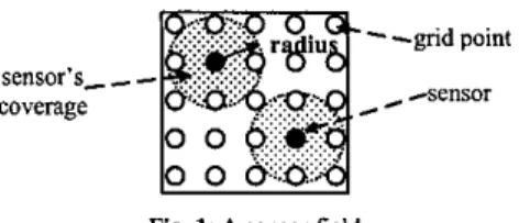
A sensor field can be represented as a collection of two- or three-dimensional grid points
[Z],
as shown in Fig. 1. A set of sensors can be deployed on the grid points to monitor the sensor field. Therefore, a target on a grid point can be located if sensors can detect the grid point.In this paper, we consider the detection model of a sensor to be a Oil coverage model. Coverage is assumed to be full (I), if the distance between the grid point and a sensor is within the transmission radius of the sensor. On the contrary, coverage will be assumed to be non- effective (0). If any grid point in a sensor field can be detected by at least one sensor, we call the field a
complete covered sensor field. In this context, a target
can be detected at any place in the field.
For any grid point, a sensor in the field can cover (1) it or not (0) is a binary variable. In addition, we defme a
power vector for each grid point. This indicates whether
sensors can cover a grid point in a field. For example, a grid point in a sensor field with 5 sensors is covered by sensors 1 and 3 and the power vector for the grid is (I, 0,
1, 0, 0). When a target appears at a grid point, the back-
end will receive reports from sensors 1 and 3, simultaneously. In a complete covered sensor field, when each grid point is identified by a unique power vector, we call the sensor field a complete discriminated sensnr field.
In this case, as soon as a target is identified in the sensor
field, the back-end is able to locate it according to the power vector of the grid.
The sensor placement for target location is to find a way to deploy sensors in a sensor field such that targets can be positioned. However, due to some resource limitations, a complete discriminated sensor field cannot be constructed. Consequently, these will be wrong determination, whenever a target occurs at any one of the grid points. Positioning accuracy, therefore, becomes
a
major issue of the problem. Distance error is one of themost natural criteria to measure positioning accuracy. The distance error of two indistinguishable grid points is
defined as the Euclidean distance between them. In this paper, we intend to minimize the distance error when complete discrimination is not possible.
3. MATHEMATICAL. MODEL
We formulate the sensor placement problem as a combinatorial optimization problem. The formulation can plan a sensor network that provides either complete, or high, discrimination depending on the cost limitation. For
Fig. 1: A sensor field
complete discrimination, it is implied that the minimum Hamming distance of power vectors for any pair of grid points will be maximized. For high discrimination, it is implied that the maximum distance error will be minimized. The problem is, therefore, defined as a min- max model.
Given Parameters:
A : {I,& ..., m) : Index set of the sensor's candidate lo~atiom
B : {I,2, ..., n ) : Index set ofthe location in the sensor field, m i n
rk : Transmission radius of sensor located at k , k E A dij ; Euclidean distance between location i and j ,
: The cost of sensor allocated at location k , k E A
i , j e B . ck
G : Total cost limitation
Decision Variables:
Yk
v j =(vi, .viz ,..., v ( ~ )
: 1, if an sensor is allocated at location k ,
k e A .
: A power vector of location i , where vjk is 1
if the target at location i can be detected by the sensor at location k and 0 otherwise.
i e B , k E A .
Objective Function and Constraints:
m
2
"fkk=l
2 1 V i e B
(K is a big number.)
Constraints (I) and (2) require the relationship between sensor transmission radius r and detection distance djk
.
If a target appears at grid point i and the grid is inside the coverage of sensor k , the target should be detected by the sensor if it is available. Constraint (3) states that the total deployment cost of sensors must limited by cost G.
Constraint (4) is the complete coverage limitation. It guarantees that any grid point in the field will be covered by at least one sensor.4. ALGORITHM
Simulated annealing (SA) is a highly reliable method for solving hard combinatorial optimization problems [5].
In the following, we use the concept of SA to derive an efficient approximate solution method for the problem.
Here, we briefly state the cooling schedule of the algorithm. Initially, we assume the sensors are deployed at all grid points. Each loop, tries to either reduce, or
interchange, a sensor randomly depending on whether the cost constraint is satisfied. For the sake of efficiency, we modify the stopping criterion. Besides frozen temperature, i f
, is reached, when both complete
coverage and discrimination are achieved as well as
z,~, =]/(I+ K ) , the procedure will then be stopped. It is not certain that the solution with complete coverage and discrimination is an optimal one. However, it is the desired solution in this problem.
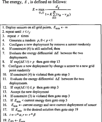
The pseudo code of the algorithm is shown as Fig. 2.
The energy, E , is defined as follows:
1. Deploy sensors on all grid points, E& t m 2. repcat until I I i f 3. repcat I times 4. 5. 6. 7. 8. 9.
10. Ifconstmint (4) is violated then goto step 3
11. Evaluate thhc energy differential AE between the two
dcploymenls.
12. If cxp(AEEI1) < p then goto step 3 13. Accept the new deployment
14. Ifconsmint (3) is violated then goto step 3
15. If Emh <current energy then goto step 3
16. Emh t current energy and save current deployment of sensor
1 I . If Emh is the desired solution then goto step 19
18. t t t . a , r t r * p
19. ZlPl t Emh
Generate a random p , 0 < p < I
Configure a new deployment by remove a sensor randomly
Ifconsmint (4) is still satisfied, then
Evaluate the energy differential AE between thc two
deployments.
If cxp(AEEI1) > p then goto step 13
Configure B n e w deployment by change a sensor to a new grid point randomly
Fig. 2: Simulated Annealing pseudo code for the sensor placement.
5. SIMULATION RESULTS
In this section, we present the simulation results. First, we evaluate the performance of the proposed algorithm in the case of smaller deployed sensor fields. The objective of the experiment is to investigate whether the algorithm can find the optimal solution under the
minimum cost limitation. Then, we show the performance results in the case of larger sensor fields under various cost limitations.
The parameters of the cooling schedule are a=0.75 and B, = 1.3 , The initial values of I and I are 5n and 0.1,
respectively; and n is the number of grids in the sensor field. The frozen temperature is set to 1/300. The K is 10000 and the cost of sensor, ci , VI i i i n
,
is set to I .As the cost of the sensor is unique, the constraint of cost limitation, Constraint (3), can be expressed by the constraint of the limitation of the number of sensors. In this section, we use a normalized term, sensor density, for the constraint. Sensor density can be defined as following:
sensor density (%) = the amount of sensors
*
100% / n5.1
Experiment I
Experiment I evaluates the performance of the proposed algorithm in the case of smaller rectangular sensor fields that have no more than 30 grid points. We compare the results with these obtained by the exhaustive search.
First, we find a minimum sensor density for a complete covered and discriminated sensor field. Then, we try to find the same result by using the proposed algorithm under the limitation of the sensor density.
Table 1 shows the results. In all cases, the proposed algorithm can achieve the same deployment for sensor fields with a minimum sensor density. The required sensor density ranges between 40% and 45%, except in the case of the 4 x 3 rectangular sensor field. The solution
time of the exhaustive search for the 1 0 x 3 sensor field is more than 65 minutes. However, the, solution can be found in 0.1 second by the proposed algorithm.
Table 1: Comparison between tho exhaustive search
Note: Opt.: by the exhaustive scarch.
5.2
Experiment I1
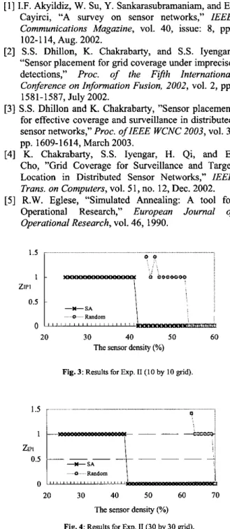
In this experiment, we consider the case of larger sensor fields that are 10x10 and 30x30 in size. Theradius of the sensor is 1. We investigate the value of zip, with various sensor densities. The results are compared with the best solution of a random placement approach. The best solution is feasible and has a minimum objective value. We first generate 1000 arbitrary solutions by the random placement approach and then pick the best one.
Fig. 3 and 4 show that the proposed algorithm can also find the desired solution when the sensor density is between 40% and 45%. This result is consistent with Table I . The solution time for a 3 0 x 3 0 sensor field is only a couple of minutes. The proposed algorithm is, therefore, very effective and scalable.
Fig. 3 and 4 indicate that sensor placement by the proposed algorithm has a minimum distance error. i.e. the distance error is 1, when the sensor density is insufficient. The random placement approach cannot achieve the same result.
The proposed algorithm can achieve a complete covered placement (i.e., the feasible solution to our
problem) under a very low sensor density. With the proposed algorithm, the minimum required sensor densities are only 25% and 24% in Fig. 3 and 4, respectively. The results are very close to the theoretical lower bound of that. (When the sensor radius is 1, a sensor can cover 5 grid points. Hence, the lower bound of sensor density for complete coverage is 20%). However, with the random placement approach, the required density for a complete covered placement is very high
(44% and 63% for Fig. 3 and 4, respectively). The experimental results show that the probability of finding the feasible solution with the random placement approach is very low when the area of the sensor field increases larger. In addition, it's very likely that this approach could find any feasible solution for a very large sensor field.
In summary, the proposed algorithm is highly scalable and robust in terms of distance error and minimum deployed density for the feasible solution.
6.
CONCLUSIONS
In this paper, we have attempted to solve the sensor placement problem. We formulated this problem as a min-max mathematical optimization model provided that either discrimination, or distance error, is the objective under cost and coverage constraints. Then, the heuristic algorithm, based on simulated annealing approach, was developed. The experimental results show that the proposed algorithm can quickly obtain an optimal solution in a small sensor field. Furthermore, the
0 Random
proposed algorithm is very effective, scalable, and robust even in large sensor fields.
References
[I] I.F. Akyildiz, W. Su, Y. Sankarasubramaniam, and E. Cayirci, "A survey on sensor networks," IEEE
Communications Magazine, vol. 40, issue: 8, pp.
102-1 14, Aug. 2002.
[2] S.S. Dhillon, K. Chakrabarty, and S.S. Iyengar,
"Sensor placement for grid coverage under imprecise detections," Proc. of the Fifth International Conference on Information Fusion, 2002, vol. 2, pp. 1581-1587, July 2002.
[3] S.S. Dhillon and K. Chakrabarty, "Sensor placement for effective coverage and surveillance in distributed sensor networks," Proc. oflEEE WCNC 2003, vol. 3,
pp. 1609-1614, March 2003.
[4] K. Chakrabarty, S.S. Iyengar, H. Qi, and E.
Cho, "Grid Coverage for Surveillance and Target Location in Distributed Sensor Networks," IEEE
Trans. on Computers, vol. 5 1, no. 12, Dec. 2002. [5] R.W. Eglese, "Simulated Annealing: A tool for
Operational Research," European Journal of
Operational Research, vol. 46, 1990.
~~ . . ~ ... ... . 0 ' . . .. . . I P e b 0 l J W ~ ZIP1
I
~I
O 5t
&-SAI
I
- - --
D Random 20 30 40 50 60 70The sensor density (%)
Fig. 4 Results for Exp 11 (30 by 30 gnd)